
Challenges and Opportunities of System-Level Prognostics


Abstract
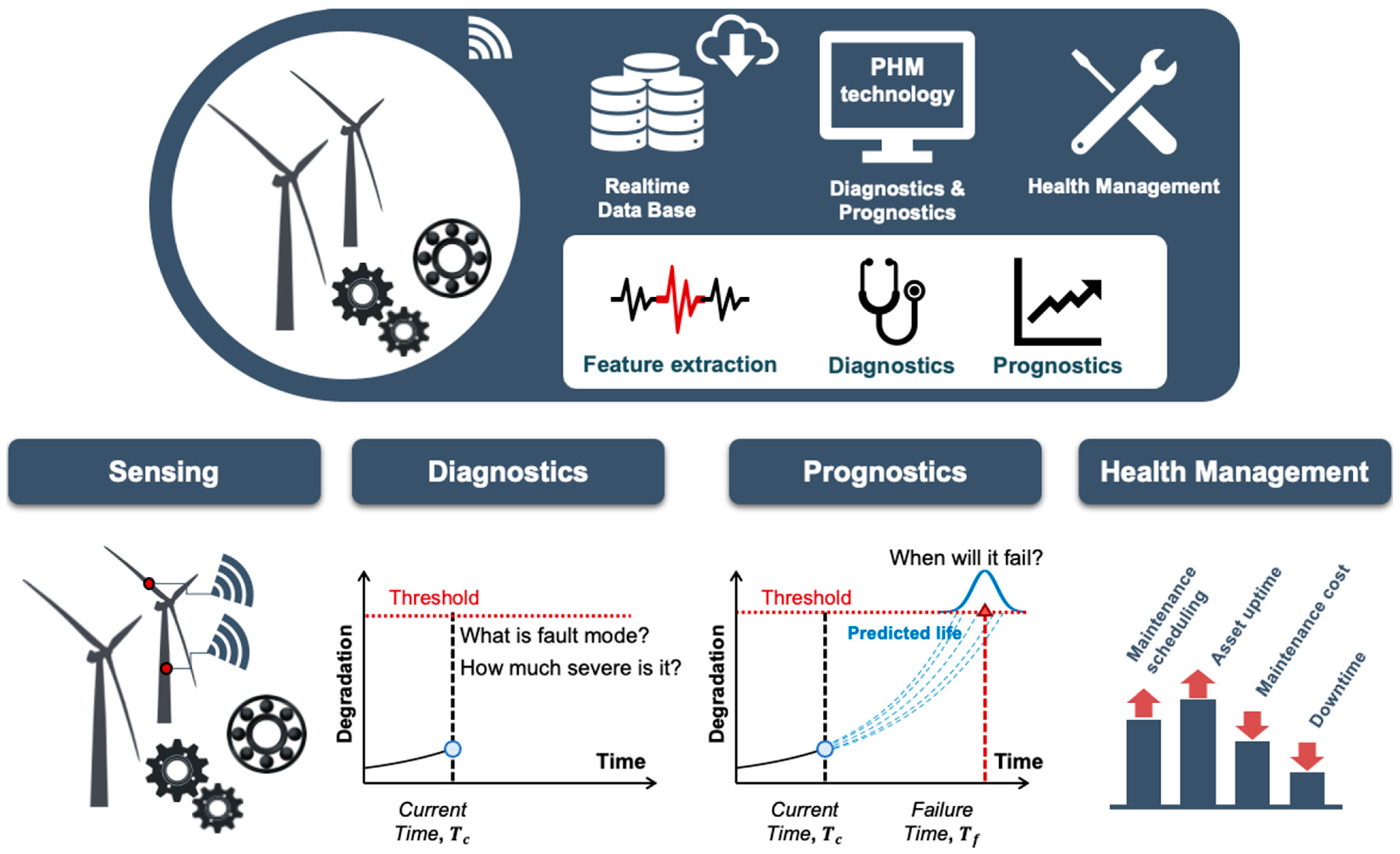
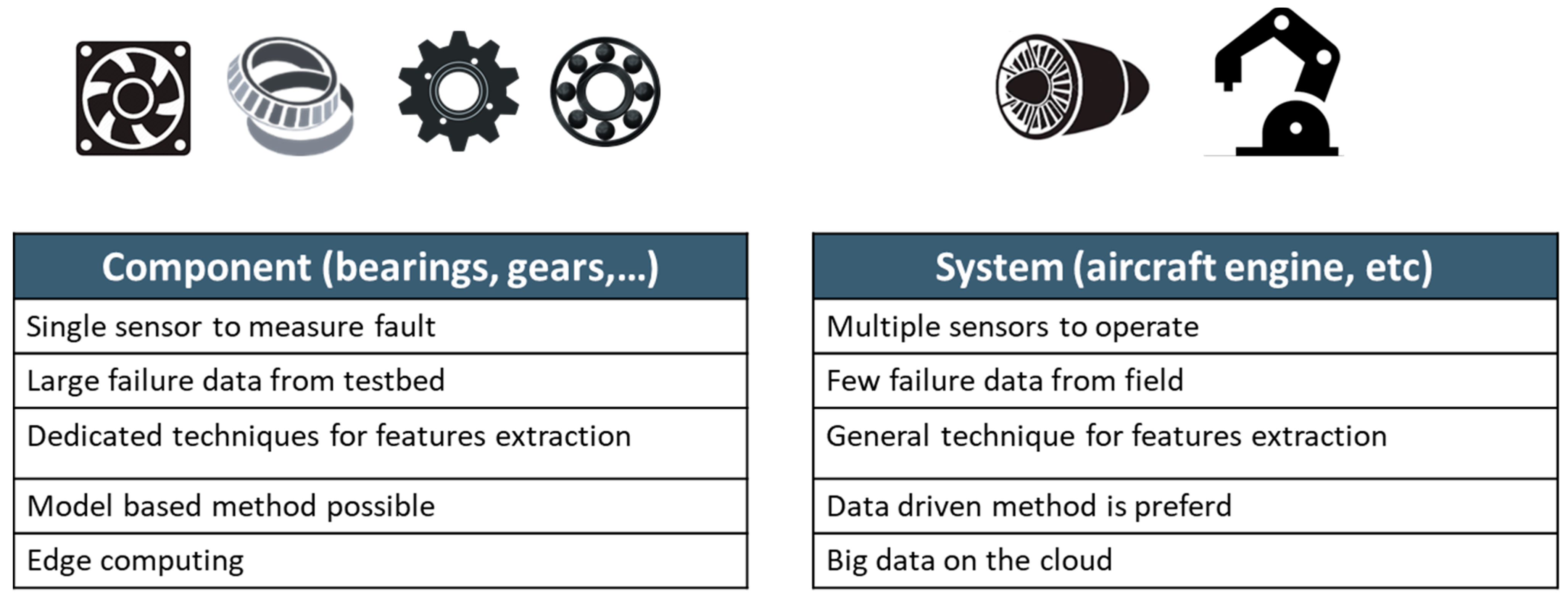
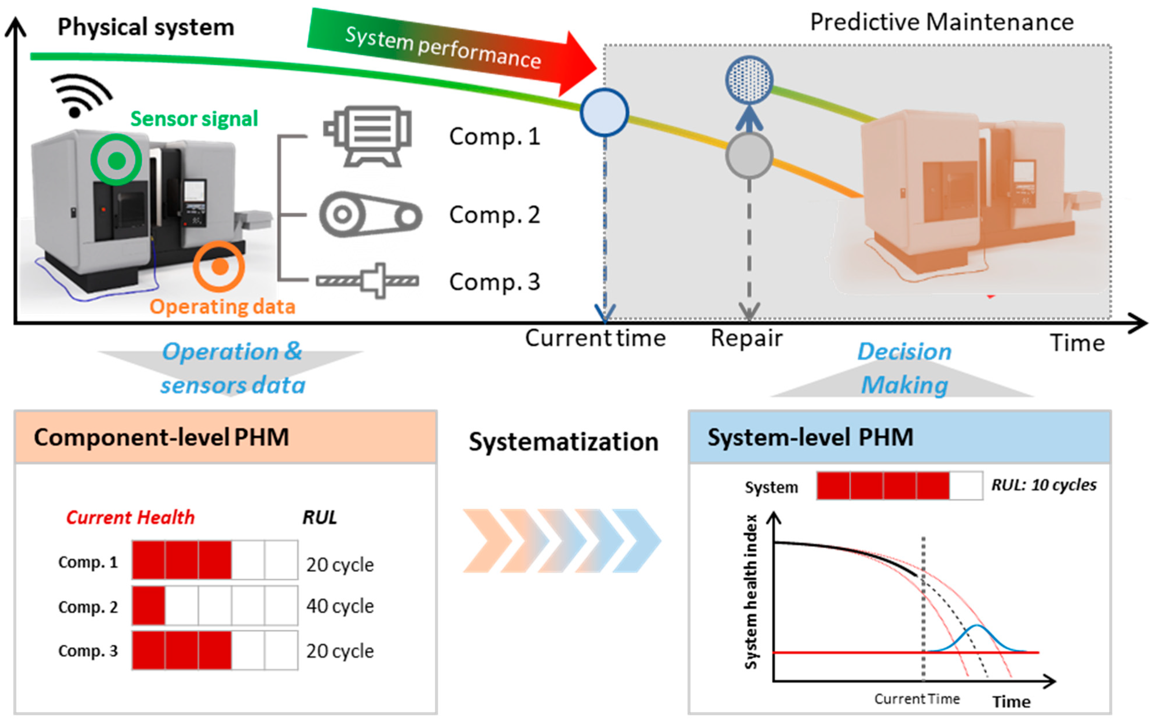
:1. Introduction
- Condition-based prognostics, not testing-based prognostics
- Health index development for multiple component systems
- Prognostics of multiple failure modes
2. Algorithms for System-Level Prognostics
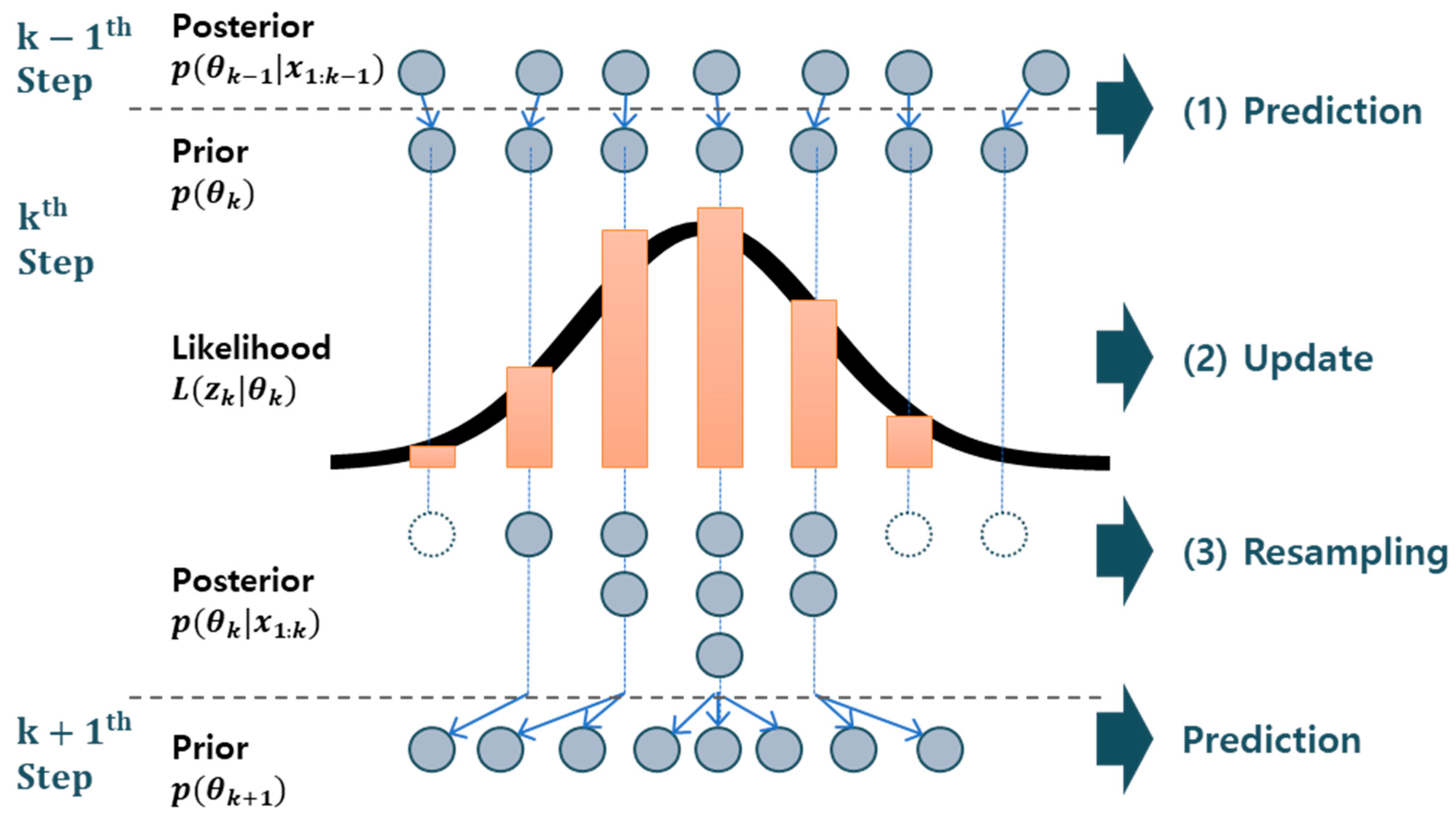
2.1. Particle Filter
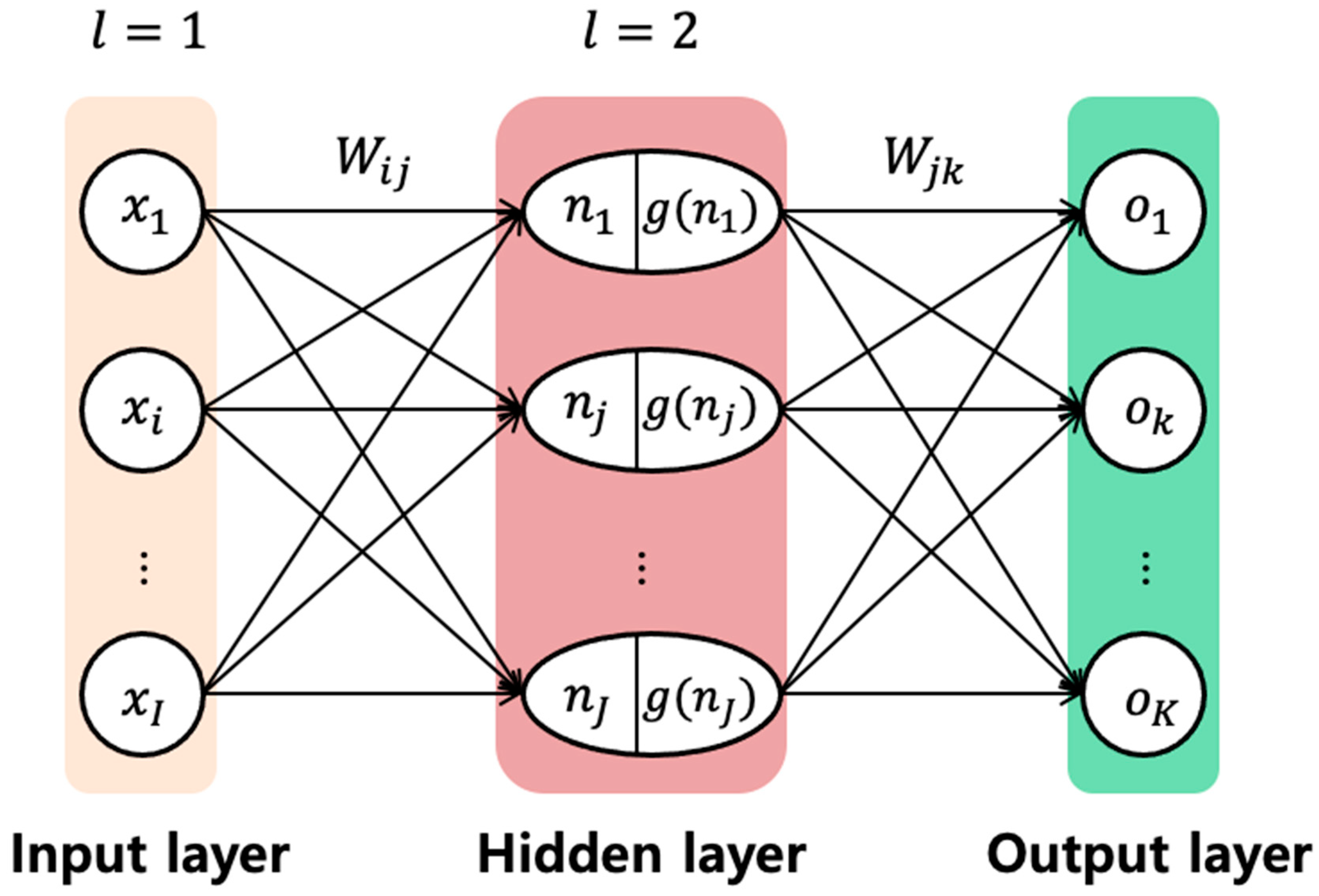
2.2. Artificial Neural Network
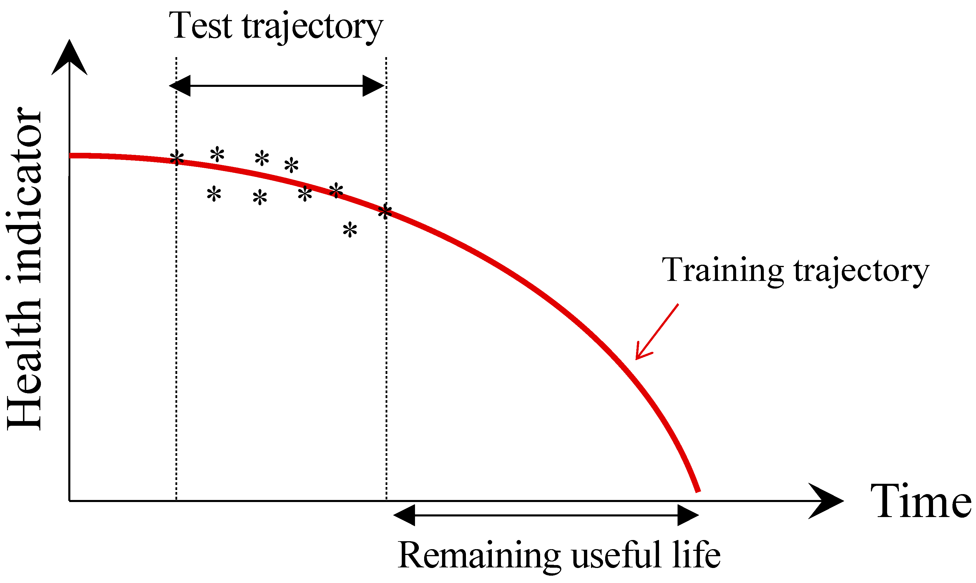
2.3. Similarity-Based Method
2.4. Cox Proportional Hazard Model
3. Approach for System-Level Prognostics
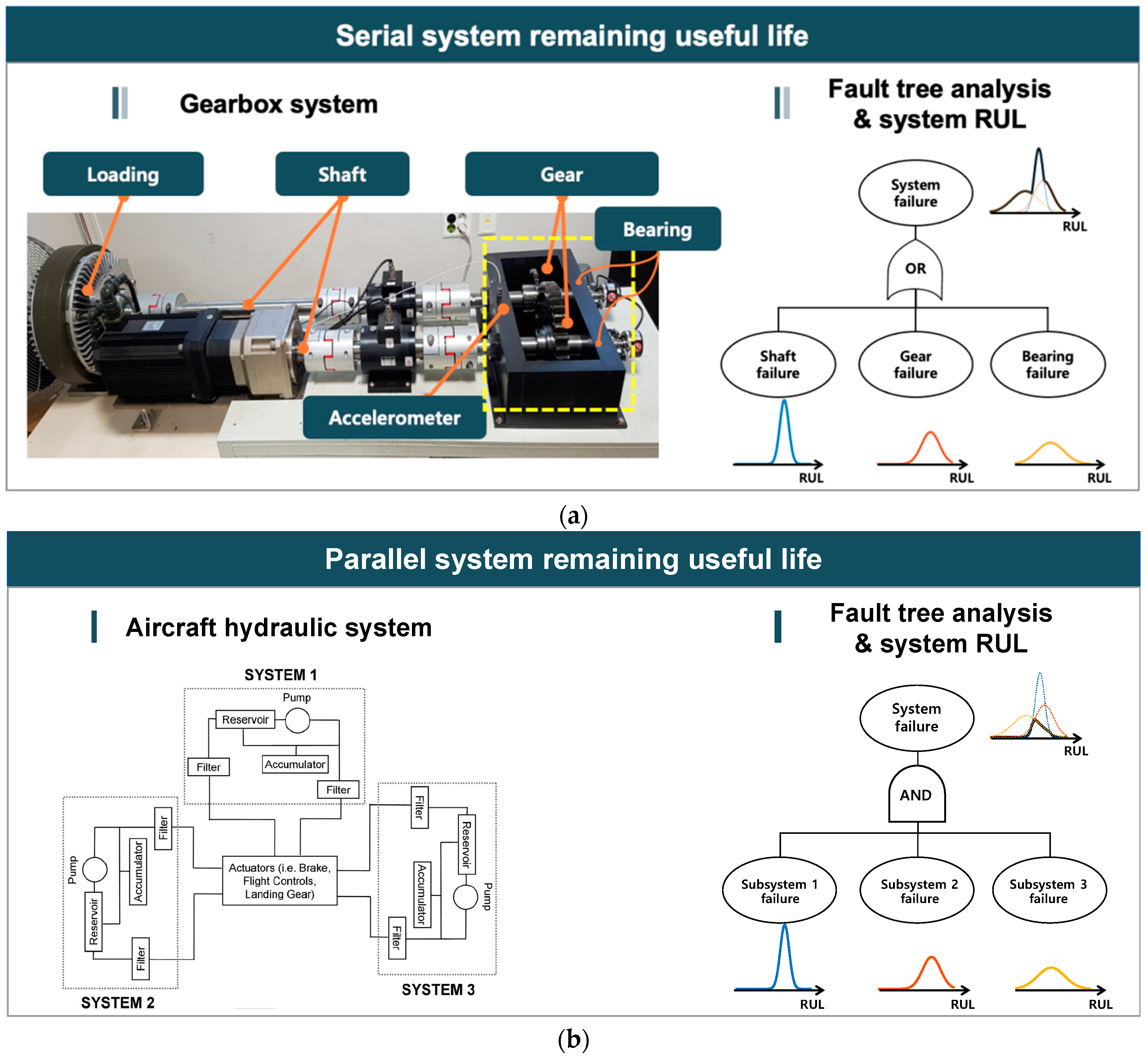
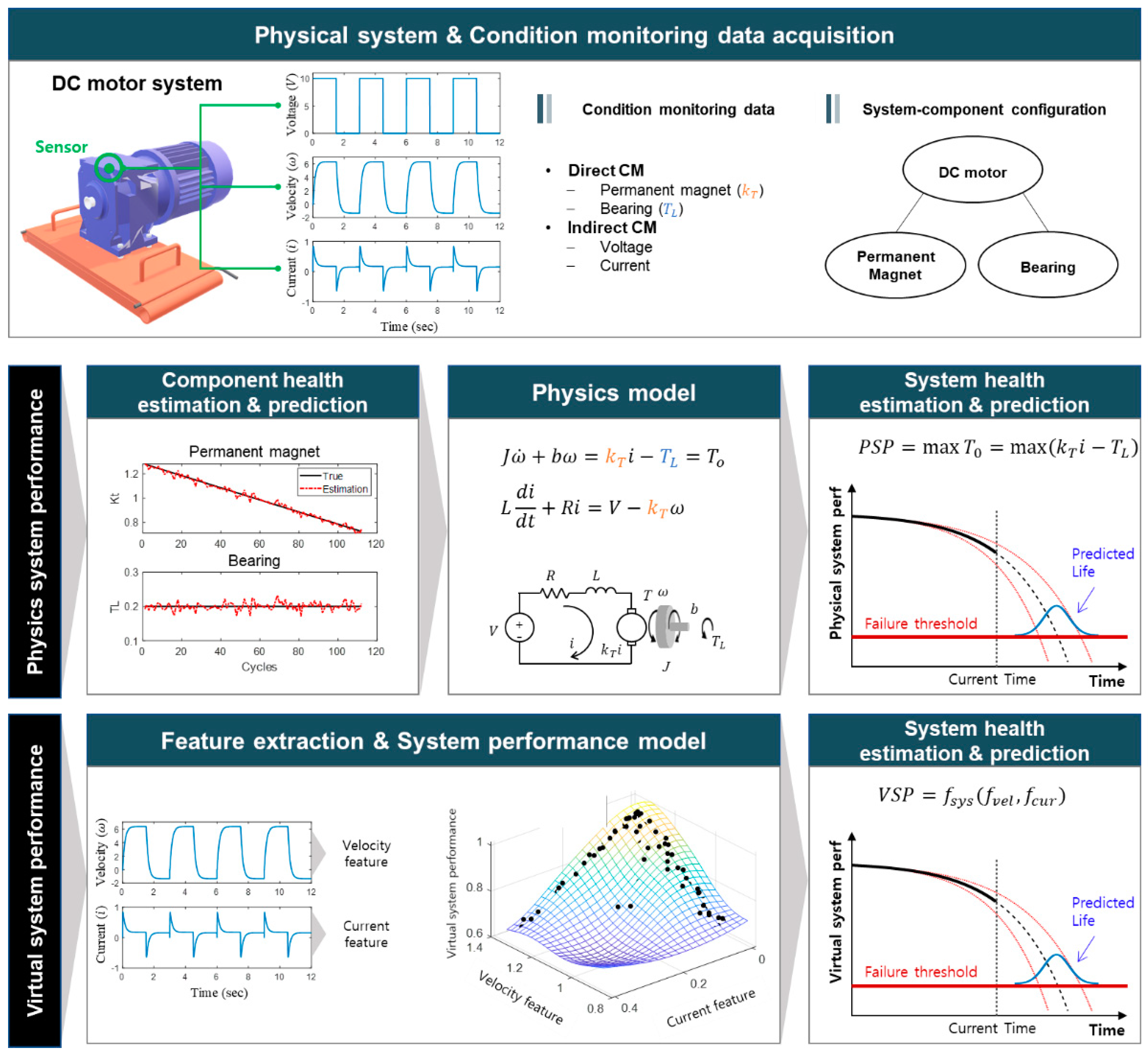
3.1. Approach 1: System Health Index-Based Approach
3.2. Approach 2: Integration of Components’ RUL into the System
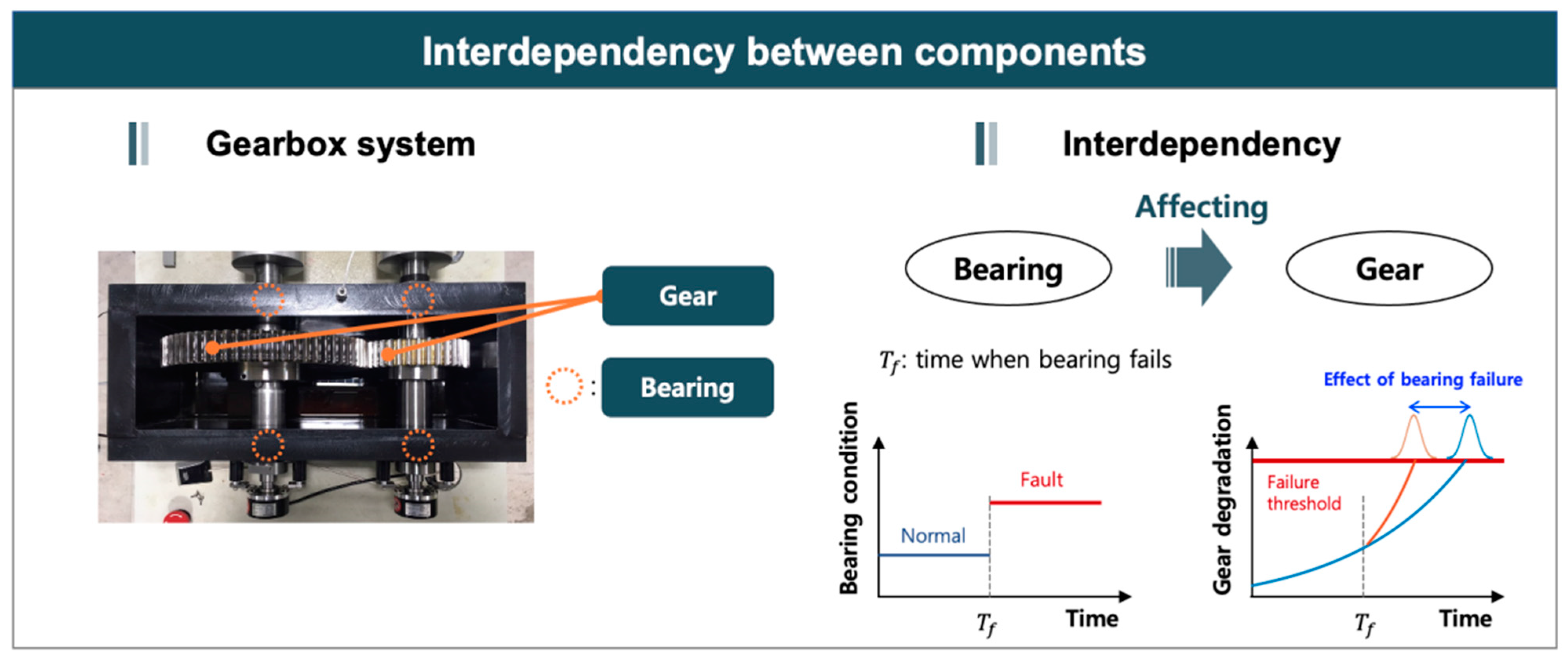
3.3. Approach 3: Prognostics under Influenced Components
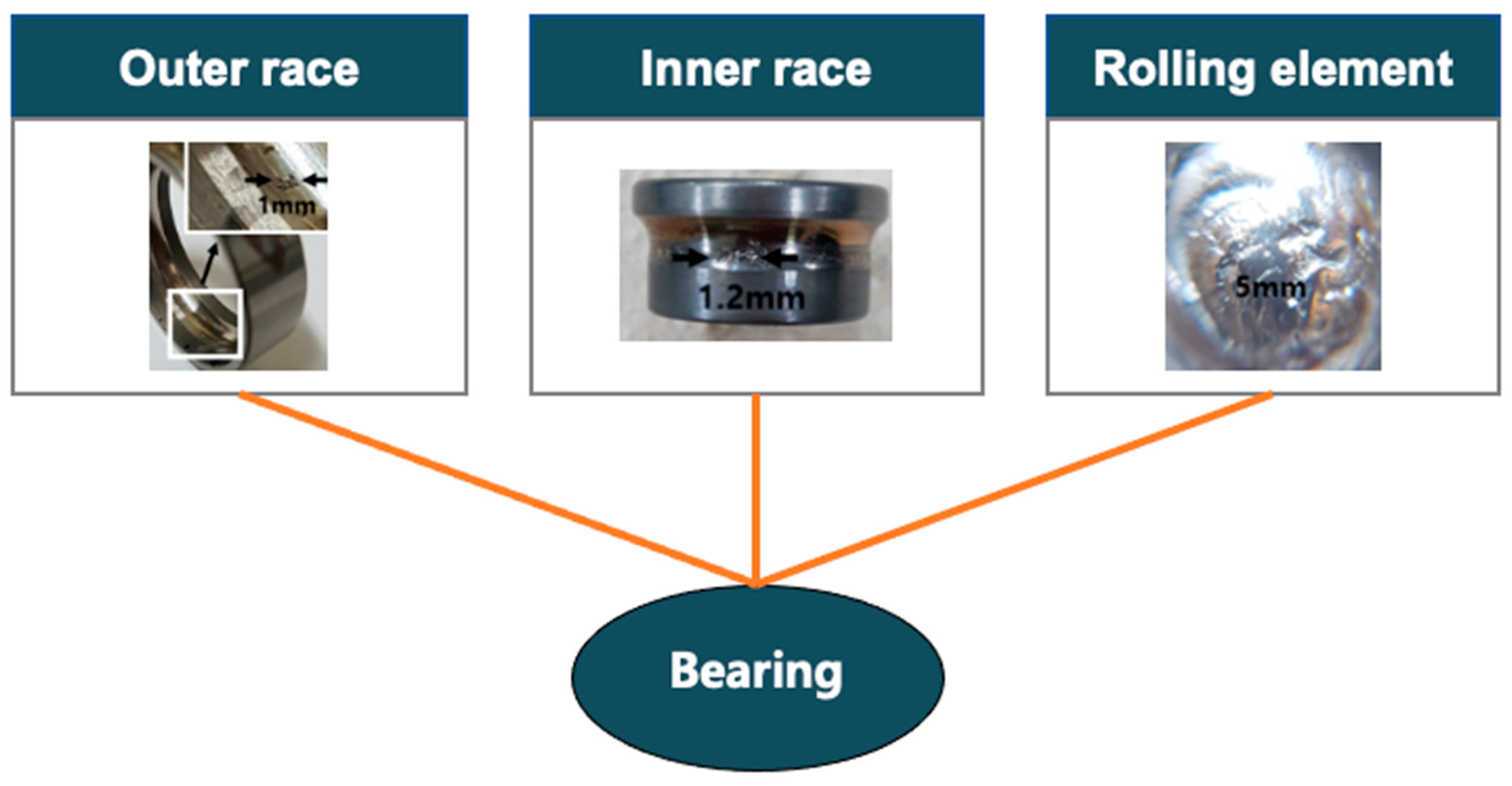
3.4. Approach 4: Prognostics of Multiple Failure Modes
4. Datasets for System-Level Prognostics
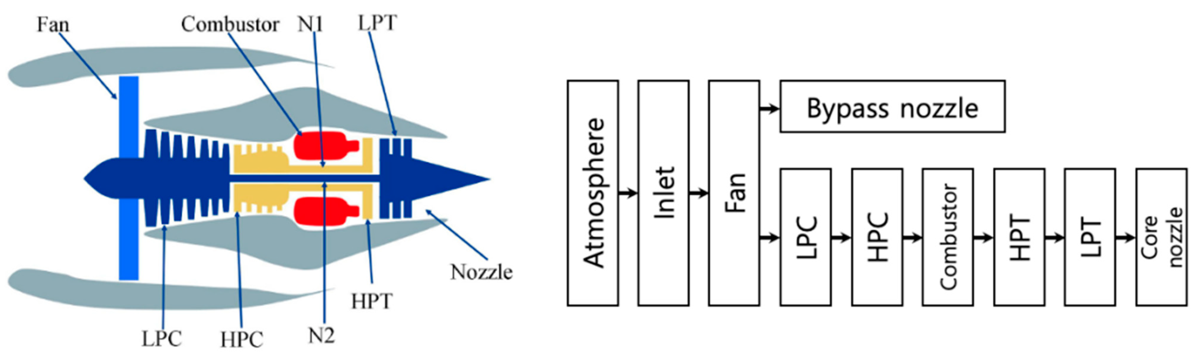
4.1. C-MAPSS Datasets
- Which fault mode of the system causes more degradation of the system?
- What is the relationship between component degradation and system performance?
- How can the failure thresholds be set for the components and system?
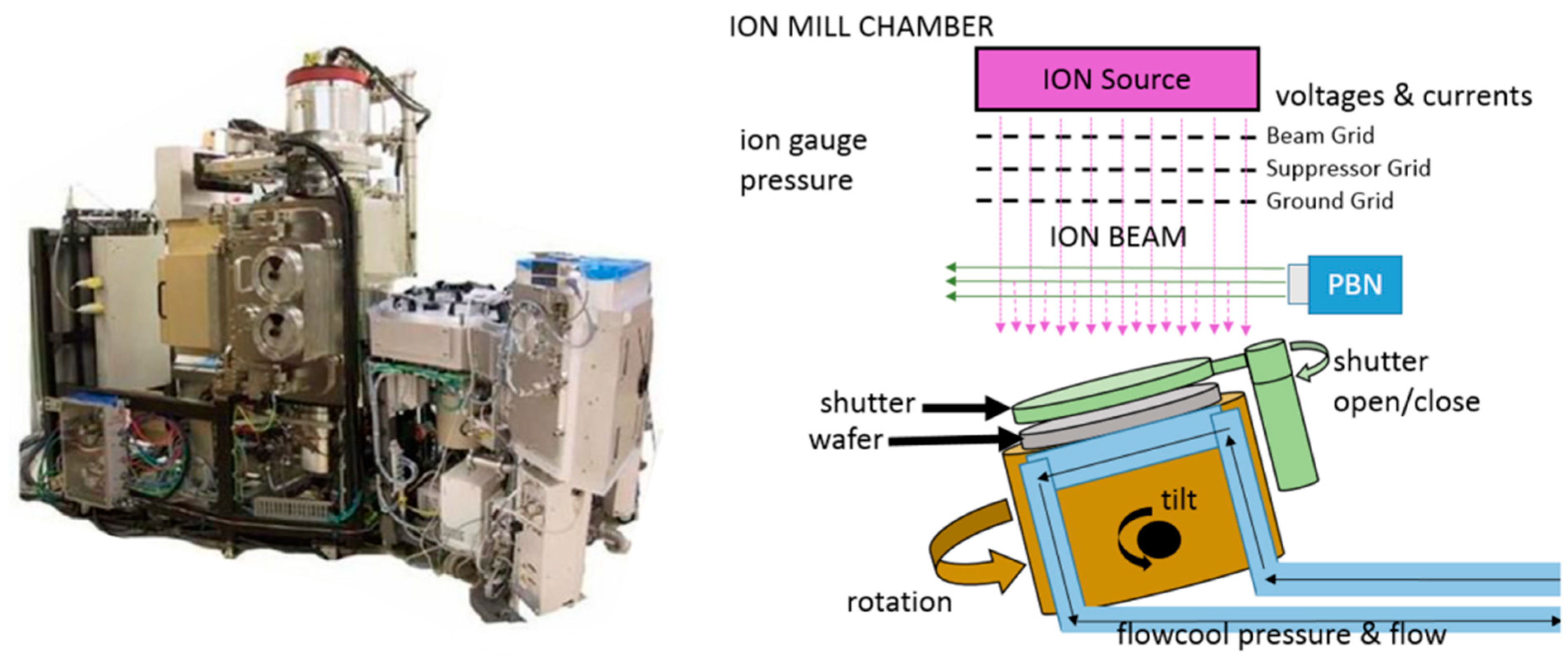
4.2. PHM Data Challenge 2018
- How to obtain a degradation model from the datasets which face three different fault modes simultaneously?
- Which fault modes are interdependent or correlated?
- How to set the appropriate thresholds for the different fault modes?
5. Challenges for Practical System-Level Prognostics
5.1. Systematization Issues in System-Level Prognostics
5.2. General Challenges for System-Level Prognostics
5.2.1. Big Data Management
5.2.2. Prognostics under Data Deficiency
5.2.3. Online Performance Assessment and Correction
5.2.4. Uncertainty Management
5.2.5. Strategy Transforming Scheduled Maintenance into Predictive Maintenance
6. Conclusions
Author Contributions
Funding
Institutional Review Board Statement
Informed Consent Statement
Data Availability Statement
Conflicts of Interest
References
- Lee, J.; Wu, F.; Zhao, W.; Ghaffari, M.; Liao, L.; Siegel, D. Prognostics and health management design for rotary machinery systems—Reviews, methodology and applications. Mech. Syst. Signal Process. 2014, 42, 314–334. [Google Scholar] [CrossRef]
- Wang, P.; Youn, B.D.; Hu, C.; Ha, J.M.; Jeon, B. A probabilistic detectability-based sensor network design method for system health monitoring and prognostics. J. Intell. Mater. Syst. Struct. 2015, 26, 1079–1090. [Google Scholar] [CrossRef]
- Angelov, P.; Giglio, V.; Guardiola, C.; Lughofer, E.; Lujan, J.M. An approach to model-based fault detection in industrial measurement systems with application to engine test benches. Meas. Sci. Technol. 2006, 17, 1809. [Google Scholar] [CrossRef]
- Zhang, S.; Zhang, S.; Wang, B.; Habetler, T.G. Deep learning algorithms for bearing fault diagnostics—A comprehensive review. IEEE Access 2020, 8, 29857–29881. [Google Scholar] [CrossRef]
- Park, Y.-J.; Fan, S.-K.S.; Hsu, C.-Y. A review on fault detection and process diagnostics in industrial processes. Processes 2020, 8, 1123. [Google Scholar] [CrossRef]
- Thoppil, N.M.; Vasu, V.; Rao, C.S.P. Deep Learning Algorithms for Machinery Health Prognostics Using Time-Series Data: A Review. J. Vib. Eng. Technol. 2021, 9, 1–23. [Google Scholar] [CrossRef]
- Sandborn, P.A.; Wilkinson, C. A maintenance planning and business case development model for the application of prognostics and health management (PHM) to electronic systems. Microelectron. Reliab. 2007, 47, 1889–1901. [Google Scholar] [CrossRef]
- Saxena, A.; Celaya, J.; Balaban, E.; Goebel, K.; Saha, B.; Saha, S.; Schwabacher, M. Metrics for evaluating performance of prognostic techniques. In Proceedings of the 2008 International Conference on Prognostics and Health Management PHM 2008, Denver, CO, USA, 6–9 October 2008. [Google Scholar]
- Jardine, A.K.S.; Lin, D.; Banjevic, D. A review on machinery diagnostics and prognostics implementing condition-based maintenance. Mech. Syst. Signal. Process. 2006, 20, 1483–1510. [Google Scholar] [CrossRef]
- Atamuradov, V.; Medjaher, K.; Dersin, P.; Lamoureux, B.; Zerhouni, N. Prognostics and health management for maintenance practitioners-review, implementation and tools evaluation. Int. J. Progn. Heal. Manag. 2017, 8, 1–31. [Google Scholar] [CrossRef]
- Coble, J.B.; Ramuhalli, P.; Bond, L.J.; Hines, W.; Upadhyaya, B. Prognostics and Health Management in Nuclear Power Plants: A Review of Technologies and Applications; U.S. Department of Energy: Washington, DC, USA, 2012. [CrossRef] [Green Version]
- Elattar, H.M.; Elminir, H.K.; Riad, A.M. Prognostics: A literature review. Complex. Intell. Syst. 2016, 2, 125–154. [Google Scholar] [CrossRef] [Green Version]
- Sun, B.; Zeng, S.; Kang, R.; Pecht, M.G. Benefits and challenges of system prognostics. IEEE Trans. Reliab. 2012, 61, 323–335. [Google Scholar] [CrossRef]
- Lei, Y.; Li, N.; Guo, L.; Li, N.; Yan, T.; Lin, J. Machinery health prognostics: A systematic review from data acquisition to RUL prediction. Mech. Syst. Signal. Process. 2018, 104, 799–834. [Google Scholar] [CrossRef]
- Shin, I.; Lee, J.; Lee, J.Y.; Jung, K.; Kwon, D.; Youn, B.D.; Jang, H.S.; Choi, J.-H. A framework for prognostics and health management applications toward smart manufacturing systems. Int. J. Precis. Eng. Manuf. Technol. 2018, 5, 535–554. [Google Scholar] [CrossRef]
- Kang, M.; Tian, J. Machine Learning: Data Pre-processing. In Prognostics and Health Management of Electronics: Fundamentals, Machine Learning, and the Internet of Things; John Wiley and Sons: Hoboken, NJ, USA, 2018; pp. 111–130. [Google Scholar]
- Bekar, E.T.; Nyqvist, P.; Skoogh, A. An intelligent approach for data pre-processing and analysis in predictive maintenance with an industrial case study. Adv. Mech. Eng. 2020, 12, 1687814020919207. [Google Scholar] [CrossRef]
- Tsui, K.L.; Chen, N.; Zhou, Q.; Hai, Y.; Wang, W. Prognostics and Health Management: A Review on Data Driven Approaches. Math. Probl. Eng. 2015, 2015, 793161. [Google Scholar] [CrossRef] [Green Version]
- Peng, Y.; Dong, M.; Zuo, M.J. Current status of machine prognostics in condition-based maintenance: A review. Int. J. Adv. Manuf. Technol. 2010, 50, 297–313. [Google Scholar] [CrossRef]
- Kan, M.S.; Tan, A.C.C.; Mathew, J. A review on prognostic techniques for non-stationary and non-linear rotating systems. Mech. Syst. Signal. Process. 2015, 62, 1–20. [Google Scholar] [CrossRef]
- Si, X.S.; Wang, W.; Hu, C.H.; Zhou, D.H. Remaining useful life estimation—A review on the statistical data driven approaches. Eur. J. Oper. Res. 2011, 213, 1–14. [Google Scholar] [CrossRef]
- An, D.; Kim, N.H.; Choi, J.H. Practical options for selecting data-driven or physics-based prognostics algorithms with reviews. Reliab. Eng. Syst. Saf. 2015, 133, 223–236. [Google Scholar] [CrossRef]
- Siegel, D.; Ly, C.; Lee, J. Methodology and framework for predicting helicopter rolling element bearing failure. IEEE Trans. Reliab. 2012, 61, 846–857. [Google Scholar] [CrossRef]
- Medjaher, K.; Tobon-Mejia, D.A.; Zerhouni, N. Remaining useful life estimation of critical components with application to bearings. IEEE Trans. Reliab. 2012, 61, 292–302. [Google Scholar] [CrossRef] [Green Version]
- He, D.; Bechhoefer, E.; Dempsey, P.; Ma, J. An integrated approach for gear health prognostics. In Proceedings of the Annual Forum Proceedings—AHS International, Fort Worth, TX, USA, 1–3 May 2012. [Google Scholar]
- Orchard, M.E.; Vachtsevanos, G.J. A particle-filtering approach for on-line fault diagnosis and failure prognosis. Trans. Inst. Meas. Control. 2009, 31, 221–246. [Google Scholar] [CrossRef]
- Saha, B.; Goebel, K.; Poll, S.; Christophersen, J. Prognostics methods for battery health monitoring using a Bayesian framework. IEEE Trans. Instrum. Meas. 2009, 58, 291–296. [Google Scholar] [CrossRef]
- Zhang, J.; Lee, J. A review on prognostics and health monitoring of Li-ion battery. J. Power Sources 2011, 196, 6007–6014. [Google Scholar] [CrossRef]
- Saha, B.; Goebel, K.; Christophersen, J. Comparison of prognostic algorithms for estimating remaining useful life of batteries. Trans. Inst. Meas. Control. 2009, 31, 293–308. [Google Scholar] [CrossRef]
- Bektas, O.; Marshall, J.; Jones, J.A. Comparison of Computational Prognostic Methods for Complex Systems under Dynamic Regimes: A Review of Perspectives. Arch. Comput. Methods Eng. 2019, 27, 999–1011. [Google Scholar] [CrossRef] [Green Version]
- Khorasgani, H.; Biswas, G.; Sankararaman, S. Methodologies for system-level remaining useful life prediction. Reliab. Eng. Syst. Saf. 2016, 154, 8–18. [Google Scholar] [CrossRef]
- Li, X.; Duan, F.; Mba, D.; Bennett, I. Rotating machine prognostics using system-level models. In Engineering Asset Management 2016; Springer: Berlin/Heidelberg, Germany, 2018; pp. 123–141. [Google Scholar]
- Saxena, A.; Sankararaman, S.; Goebel, K. Performance Evaluation for Fleet-based and Unit-based Prognostic Methods. In Proceedings of the Second European Conference of the Prognostics and Health Management Society, Nantes, France, 8–10 July 2014. [Google Scholar]
- Sankararaman, S. Remaining useful life prediction through failure probability computation for conditioned-based prognostics. In Proceedings of the Annual Conference of the Prognostics and Health Management Society, Coronado, CA, USA, 18–24 October 2015. [Google Scholar]
- Paris, P.C.; Erdogan, F. A Critical Analysis of Crack Propagation Laws. J. Basic Eng. 1960, 85, 528–534. [Google Scholar] [CrossRef]
- Huang, X.; Torgeir, M.; Cui, W. An engineering model of fatigue crack growth under variable amplitude loading. Int. J. Fatigue 2008, 30, 2–10. [Google Scholar] [CrossRef]
- An, D.; Choi, J.H.; Kim, N.H. Prognostics 101: A tutorial for particle filter-based prognostics algorithm using Matlab. Reliab. Eng. Syst. Saf. 2013, 115, 161–169. [Google Scholar] [CrossRef]
- Bechhoefer, E. A method for generalized prognostics of a component using Paris Law. In Proceedings of the Annual Forum Proceedings—AHS International, Montreal, CA, USA, 29 April–1 May 2008. [Google Scholar]
- Peel, L. Data driven prognostics using a Kalman filter ensemble of neural network models. In Proceedings of the 2008 International Conference on Prognostics and Health Management, Denver, CO, USA, 6–9 October 2008. [Google Scholar]
- Heimes, F.O. Recurrent Neural Networks for Remaining Useful Life Estimation. In Proceedings of the 2008 International Conference on Prognostics and Health Management, Denver, CO, USA, 6–9 October 2008. [Google Scholar] [CrossRef]
- Babu, G.S.; Zhao, P.; Li, X.-L. Deep convolutional neural network based regression approach for estimation of remaining useful life. In Proceedings of the International Conference on Database Systems for Advanced Applications, Dallas, TX, USA, 16–19 April 2016; Springer: Berlin/Heidelberg, Germany, 2016; pp. 214–228. [Google Scholar]
- Zheng, S.; Ristovski, K.; Farahat, A.; Gupta, C. Long short-term memory network for remaining useful life estimation. In Proceedings of the Prognostics and Health Management (ICPHM), Piscataway, NJ, USA, 19–21 June 2017; pp. 88–95. [Google Scholar]
- Vachtsevanos, G.J.; Vachtsevanos, G.J. Intelligent Fault Diagnosis and Prognosis for Engineering Systems; Wiley Online Library: Hoboken, NJ, USA, 2006; Volume 456. [Google Scholar]
- Caesarendra, W.; Niu, G.; Yang, B.-S. Machine condition prognosis based on sequential Monte Carlo method. Expert Syst. Appl. 2010, 37, 2412–2420. [Google Scholar] [CrossRef]
- Kim, S.; Park, H.J.; Choi, J.-H.; Kwon, D. A novel prognostics approach using shifting kernel particle filter of Li-ion batteries under state changes. IEEE Trans. Ind. Electron. 2020, 68, 3485–3493. [Google Scholar] [CrossRef]
- Hsu, C.S.; Jiang, J.R. Remaining useful life estimation using long short-term memory deep learning. In Proceedings of the 4th IEEE International Conference on Applied System Innovation 2018, ICASI 2018, Tokyo, Japan, 13–17 April 2018. [Google Scholar]
- Bektas, O.; Jones, J.A.; Sankararaman, S.; Roychoudhury, I.; Goebel, K. A neural network filtering approach for similarity-based remaining useful life estimation. Int. J. Adv. Manuf. Technol. 2019, 101, 87–103. [Google Scholar] [CrossRef] [Green Version]
- Widodo, A.; Yang, B.-S. Machine health prognostics using survival probability and support vector machine. Expert Syst. Appl. 2011, 38, 8430–8437. [Google Scholar] [CrossRef]
- Widodo, A.; Yang, B.-S. Application of relevance vector machine and survival probability to machine degradation assessment. Expert Syst. Appl. 2011, 38, 2592–2599. [Google Scholar] [CrossRef]
- Caesarendra, W.; Widodo, A.; Yang, B.-S. Combination of probability approach and support vector machine towards machine health prognostics. Probabilistic Eng. Mech. 2011, 26, 165–173. [Google Scholar] [CrossRef]
- Pham, H.T.; Yang, B.-S.; Nguyen, T.T. Machine performance degradation assessment and remaining useful life prediction using proportional hazard model and support vector machine. Mech. Syst. Signal. Process. 2012, 32, 320–330. [Google Scholar]
- Sun, J.; Zuo, H.; Wang, W.; Pecht, M.G. Application of a state space modeling technique to system prognostics based on a health index for condition-based maintenance. Mech. Syst. Signal. Process. 2012, 28, 585–596. [Google Scholar] [CrossRef]
- Messai, A.; Mellit, A.; Abdellani, I.; Massi Pavan, A. On-line fault detection of a fuel rod temperature measurement sensor in a nuclear reactor core using ANNs. Prog. Nucl. Energy 2015, 79, 8–21. [Google Scholar] [CrossRef]
- Zhang, A.; Wang, H.; Li, S.; Cui, Y.; Liu, Z.; Yang, G.; Hu, J. Transfer learning with deep recurrent neural networks for remaining useful life estimation. Appl. Sci. 2018, 8, 2416. [Google Scholar] [CrossRef] [Green Version]
- Li, X.; Ding, Q.; Sun, J.Q. Remaining useful life estimation in prognostics using deep convolution neural networks. Reliab. Eng. Syst. Saf. 2018, 172, 1–11. [Google Scholar] [CrossRef] [Green Version]
- Wu, Y.; Yuan, M.; Dong, S.; Lin, L.; Liu, Y. Remaining useful life estimation of engineered systems using vanilla LSTM neural networks. Neurocomputing 2018, 275, 167–179. [Google Scholar] [CrossRef]
- Liu, J.; Djurdjanovic, D.; Ni, J.; Casoetto, N.; Lee, J. Similarity based method for manufacturing process performance prediction and diagnosis. Comput. Ind. 2007, 58, 558–566. [Google Scholar] [CrossRef]
- Wang, T. Trajectory Similarity Based Prediction for Remaining Useful Life Estimation. Ph.D. Thesis, University of Cincinnati, Cincinnati, OH, USA, 2010. [Google Scholar]
- Eker, O.F.; Camci, F.; Jennions, I.K. A Similarity-based Prognostics Approach for Remaining Useful Life Prediction. In Proceedings of the Second European Conference of the Prognostics and Health Management Society, Nantes, France, 8–10 July 2014. [Google Scholar]
- Khelif, R.; Malinowski, S.; Chebel-Morello, B.; Zerhouni, N. RUL prediction based on a new similarity-instance based approach. In Proceedings of the IEEE International Symposium on Industrial Electronics, Istanbul, Turkey, 1–4 June 2014. [Google Scholar]
- Lam, J.; Sankararaman, S.; Stewart, B. Enhanced trajectory based similarity prediction with uncertainty quantification. In Proceedings of the PHM 2014—Proceedings of the Annual Conference of the Prognostics and Health Management Society 2014, Fort Worth, TX, USA, 29 September–2 October 2014. [Google Scholar]
- Cox, D.R. Regression Models and Life-Tables. J. R. Stat. Soc. Ser. B 1972, 34, 187–202. [Google Scholar] [CrossRef]
- Sun, Y.; Ma, L.; Mathew, J.; Wang, W.; Zhang, S. Mechanical systems hazard estimation using condition monitoring. Mech. Syst. Signal. Process. 2006, 20, 1189–1201. [Google Scholar] [CrossRef]
- Rodrigues, L.R. Remaining useful life prediction for multiple-component systems based on a system-level performance indicator. IEEE ASME Trans. Mechatron. 2017, 23, 141–150. [Google Scholar] [CrossRef]
- Wang, J.B.; Wang, X.H.; Wang, L.Z. Modeling of BN lifetime prediction of a system based on integrated multi-level information. Sensors 2017, 17, 2123. [Google Scholar] [CrossRef] [PubMed] [Green Version]
- Liu, Y.; Zuo, M.J.; Li, Y.F.; Huang, H.Z. Dynamic Reliability Assessment for Multi-State Systems Utilizing System-Level Inspection Data. IEEE Trans. Reliab. 2015, 64, 1287–1299. [Google Scholar] [CrossRef]
- Yan, J.; Koç, M.; Lee, J. A prognostic algorithm for machine performance assessment and its application. Prod. Plan. Control. 2004, 15, 796–801. [Google Scholar] [CrossRef]
- Wang, T.; Yu, J.; Siegel, D.; Lee, J. A similarity-based prognostics approach for remaining useful life estimation of engineered systems. In Proceedings of the 2008 International Conference on Prognostics and Health Management PHM 2008, Denver, CO, USA, 6–9 October 2008. [Google Scholar]
- Zhang, W.; Liu, J.; Gao, M.; Pan, C.; Huusom, J.K. A fault early warning method for auxiliary equipment based on multivariate state estimation technique and sliding window similarity. Comput. Ind. 2019, 107, 67–80. [Google Scholar] [CrossRef]
- Garvey, D.; Garvey, J.; Seibert, R.; Hines, J.W.; Arndt, S.A. Application of on-line monitoring techniques to nuclear plant data. In Proceedings of the 5th International Topical Meeting on Nuclear Plant Instrumentation Controls, and Human Machine Interface Technology (NPIC and HMIT 2006), Albuquerque, NM, USA, 12–16 November 2006. [Google Scholar]
- Coble, J.; Hines, J.W. Applying the general path model to estimation of remaining useful life. Int. J. Progn. Heal. Manag. 2011, 2, 71–82. [Google Scholar]
- Riad, A.M.; Elminir, H.K.; Elattar, H.M. Evaluation of neural networks in the subject of prognostics as compared to linear regression model. Int. J. Eng. Technol. 2010, 10, 52–58. [Google Scholar]
- Abbas, M. System Level Health Assessment of Complex Engineered Processes. Ph.D. Thesis, Georgia Institute of Technology, Atlanta, GA, USA, 2010. [Google Scholar]
- Wen, L.; Dong, Y.; Gao, L. A new ensemble residual convolutional neural network for remaining useful life estimation. Math. Biosci. Eng. 2019, 16, 862–880. [Google Scholar] [CrossRef]
- Li, H.; Zhao, W.; Zhang, Y.; Zio, E. Remaining useful life prediction using multi-scale deep convolutional neural network. Appl. Soft Comput. 2020, 89, 106113. [Google Scholar] [CrossRef]
- Behera, S.; Misra, R.; Sillitti, A. Multiscale deep bidirectional gated recurrent neural networks based prognostic method for complex non-linear degradation systems. Inf. Sci. 2021, 554, 120–144. [Google Scholar] [CrossRef]
- Hu, C.; Youn, B.D.; Wang, P.; Taek Yoon, J. Ensemble of data-driven prognostic algorithms for robust prediction of remaining useful life. Reliab. Eng. Syst. Saf. 2012, 103, 120–135. [Google Scholar] [CrossRef] [Green Version]
- Zhang, Q.; Tse, P.W.T.; Wan, X.; Xu, G. Remaining useful life estimation for mechanical systems based on similarity of phase space trajectory. Expert Syst. Appl. 2015, 42, 2353–2360. [Google Scholar] [CrossRef]
- Muller, A.; Suhner, M.C.; Iung, B. Formalisation of a new prognosis model for supporting proactive maintenance implementation on industrial system. Reliab. Eng. Syst. Saf. 2008, 93, 234–253. [Google Scholar] [CrossRef]
- Loukopoulos, P.; Zolkiewski, G.; Bennett, I.; Sampath, S.; Pilidis, P.; Duan, F.; Sattar, T.; Mba, D. Reciprocating compressor prognostics of an instantaneous failure mode utilising temperature only measurements. Appl. Acoust. 2019, 147, 77–86. [Google Scholar] [CrossRef]
- Park, H.J.; Kim, S.; Han, S.-Y.; Ham, S.; Park, K.J.; Choi, J.-H. Machine Health Assessment Based on an Anomaly Indicator Using a Generative Adversarial Network. Int. J. Precis. Eng. Manuf. 2021, 22, 1–12. [Google Scholar] [CrossRef]
- Jiao, R.; Peng, K.; Dong, J.; Zhang, C. Fault monitoring and remaining useful life prediction framework for multiple fault modes in prognostics. Reliab. Eng. Syst. Saf. 2020, 203, 107028. [Google Scholar] [CrossRef]
- Xu, J.; Wang, Y.; Xu, L. PHM-oriented integrated fusion prognostics for aircraft engines based on sensor data. IEEE Sens. J. 2013, 14, 1124–1132. [Google Scholar] [CrossRef]
- Booyse, W.; Wilke, D.N.; Heyns, S. Deep digital twins for detection, diagnostics and prognostics. Mech. Syst. Signal. Process. 2020, 140, 106612. [Google Scholar] [CrossRef]
- Gomes, J.P.P.; Rodrigues, L.R.; Galvão, R.K.H.; Yoneyama, T. System level RUL estimation for multiple-component systems. In Proceedings of the Annual Conference of the Prognostics and Health Management Society, New Orleans, FL, USA, 14–17 October 2013; pp. 74–82. [Google Scholar]
- Ferri, F.A.S.; Rodrigues, L.R.; Gomes, J.P.P.; De Medeiros, I.P.; Galvao, R.K.H.; Nascimento, C.L. Combining PHM information and system architecture to support aircraft maintenance planning. In Proceedings of the SysCon 2013—7th Annual IEEE International Systems Conference Proceedings, Orlando, FL, USA, 15–18 April 2013. [Google Scholar]
- Daigle, M.; Bregon, A.; Roychoudhury, I. A Distributed Approach to System-Level Prognostics; National Aeronautics and Space Administration Moffett Field Ca Ames Research: Mountain View, CA, USA, 2012.
- Daigle, M.J.; Bregon, A.; Roychoudhury, I. Distributed prognostics based on structural model decomposition. IEEE Trans. Reliab. 2014, 63, 495–510. [Google Scholar] [CrossRef] [Green Version]
- Daigle, M.; Sankararaman, S.; Roychoudhury, I. System-level Prognostics for the National Airspace. In Proceedings of the Annual Conference of the Prognostics and Health Management Society, Denver, CO, USA, 3–6 October 2016. [Google Scholar]
- Daigle, M.; Goebel, K. Multiple damage progression paths in model-based prognostics. In Proceedings of the IEEE Aerospace Conference Proceedings, Big Sky, MT, USA, 5–12 March 2011. [Google Scholar]
- Vasan, A.S.S.; Chen, C.; Pecht, M. A circuit-centric approach to electronic system-level diagnostics and prognostics. In Proceedings of the PHM 2013—2013 IEEE International Conference on Prognostics and Health Management, Gaithersburg, MD, USA, 24–27 June 2013. [Google Scholar]
- Chiachio, M.; Chiachio, J.; Sankararaman, S.; Andrews, J. Integration of prognostics at a system level: A Petri net approach. In Proceedings of the Annual Conference Of The PHM Society, St. Petersburg, FL, USA, 2–5 October 2017. [Google Scholar]
- Vianna, W.O.L.; Yoneyama, T. Predictive maintenance optimization for aircraft redundant systems subjected to multiple wear profiles. IEEE Syst. J. 2017, 12, 1170–1181. [Google Scholar] [CrossRef]
- Rodrigues, L.R.; Gomes, J.P.P.; Ferri, F.A.S.; Medeiros, I.P.; Galvao, R.K.H.; Nascimento, C.L., Jr. Use of PHM Information and System Architecture for Optimized Aircraft Maintenance Planning. IEEE Syst. J. 2015, 9, 1197–1207. [Google Scholar] [CrossRef]
- Al-Mohamad, A.; Hoblos, G.; Puig, V. A hybrid system-level prognostics approach with online RUL forecasting for electronics-rich systems with unknown degradation behaviors. Microelectron. Reliab. 2020, 111, 113676. [Google Scholar] [CrossRef]
- Olde Keizer, M.C.A.; Flapper, S.D.P.; Teunter, R.H. Condition-based maintenance policies for systems with multiple dependent components: A review. Eur. J. Oper. Res. 2017, 261, 405–420. [Google Scholar] [CrossRef]
- Tamssaouet, F.; Nguyen, K.T.P.; Medjaher, K.; Orchard, M.E. Degradation Modeling and Uncertainty Quantification for System-Level Prognostics. IEEE Syst. J. 2020, 15, 1628–1639. [Google Scholar] [CrossRef]
- Tamssaouet, F.; Nguyen, K.T.P.; Medjaher, K. System-Level Prognostics Under Mission Profile Effects Using Inoperability Input-Output Model. IEEE Trans. Syst. Man Cybern. Syst. 2019, 51, 4659–4669. [Google Scholar] [CrossRef]
- Tamssaouet, F.; Nguyen, T.P.K.; Medjaher, K.; Orchard, M.E. Uncertainty Quantification in System-level Prognostics: Application to Tennessee Eastman Process. In Proceedings of the 6th International Conference on Control, Decision and Information Technologies (CoDIT), Paris, France, 23–26 April 2019; pp. 1243–1248. [Google Scholar]
- Tamssaouet, F.; Nguyen, T.P.K.; Medjaher, K. System-level prognostics based on inoperability input-output model. In Proceedings of the Annual Conference of the PHM Society, Philadelphia, PA, USA, 24–27 September 2018. [Google Scholar]
- Tamssaouet, F.; Nguyen, K.T.P.; Medjaher, K.; Orchard, M.E. Online joint estimation and prediction for system-level prognostics under component interactions and mission profile effects. ISA Trans. 2020, 113, 52–63. [Google Scholar] [CrossRef]
- Tamssaouet, F.; Nguyen, K.T.P.; Medjaher, K. System Remaining Useful Life Maximization through Mission Profile Optimization. In Proceedings of the Asia-Pacific Conference of the Prognostics and Health Management Society, Bejing, China, 22–24 July 2019. [Google Scholar]
- Liu, J.; Zio, E. System dynamic reliability assessment and failure prognostics. Reliab. Eng. Syst. Saf. 2017, 160, 21–36. [Google Scholar] [CrossRef] [Green Version]
- Hu, J.; Zhang, L.; Tian, W.; Zhou, S. DBN based failure prognosis method considering the response of protective layers for the complex industrial systems. Eng. Fail. Anal. 2017, 79, 504–519. [Google Scholar] [CrossRef]
- Maitre, J.; Gupta, J.S.; Medjaher, K.; Zerhouni, N. A PHM system approach: Application to a simplified aircraft bleed system. In Proceedings of the IEEE Aerospace Conference Proceedings, Big Sky, MT, USA, 5–12 March 2016. [Google Scholar]
- Hafsa, W.; Chebel-Morello, B.; Varnier, C.; Medjaher, K.; Zerhouni, N. Prognostics of health status of multi-component systems with degradation interactions. In Proceedings of the Proceedings of International Conference on Industrial Engineering and Systems Management IEEE IESM 2015, Seville, Spain, 21–23 October 2015. [Google Scholar]
- Hanwen, Z.; Maoyin, C.; Donghua, Z. Remaining useful life prediction for a nonlinear multi-degradation system with public noise. J. Syst. Eng. Electron. 2018, 29, 429–435. [Google Scholar]
- Bian, L.; Gebraeel, N. Stochastic framework for partially degradation systems with continuous component degradation-rate-interactions. Nav. Res. Logist. 2014, 61, 286–303. [Google Scholar] [CrossRef]
- Bian, L.; Gebraeel, N. Stochastic modeling and real-time prognostics for multi-component systems with degradation rate interactions. IIE Trans. Institute Ind. Eng. 2014, 46, 470–482. [Google Scholar] [CrossRef]
- Lin, Y.-H.; Li, Y.-F.; Zio, E. A reliability assessment framework for systems with degradation dependency by combining binary decision diagrams and Monte Carlo simulation. IEEE Trans. Syst. Man, Cybern. Syst. 2015, 46, 1556–1564. [Google Scholar] [CrossRef]
- Lin, Y.-H.; Li, Y.-F.; Zio, E. Component importance measures for components with multiple dependent competing degradation processes and subject to maintenance. IEEE Trans. Reliab. 2015, 65, 547–557. [Google Scholar] [CrossRef]
- Prakash, O.; Samantaray, A.K.; Bhattacharyya, R. Model-based multi-component adaptive prognosis for hybrid dynamical systems. Control. Eng. Pract. 2018, 72, 1–18. [Google Scholar] [CrossRef]
- Li, X.; Makis, V.; Zhao, Z.; Zuo, H.; Duan, C.; Zhang, Y. Optimal Bayesian maintenance policy for a gearbox subject to two dependent failure modes. Qual. Reliab. Eng. Int. 2019, 35, 659–676. [Google Scholar] [CrossRef]
- Rasmekomen, N.; Parlikad, A.K. Condition-based maintenance of multi-component systems with degradation state-rate interactions. Reliab. Eng. Syst. Saf. 2016, 148, 1–10. [Google Scholar] [CrossRef]
- Nguyen, K.-A.; Do, P.; Grall, A. Condition-based maintenance for multi-component systems using importance measure and predictive information. Int. J. Syst. Sci. Oper. Logist. 2014, 1, 228–245. [Google Scholar] [CrossRef]
- Ragab, A.; Yacout, S.; Ouali, M.S.; Osman, H. Multiple failure modes prognostics using logical analysis of data. In Proceedings of the Annual Reliability and Maintainability Symposium, Palm Harbor, FL, USA, 26–29 January 2015. [Google Scholar]
- Sankavaram, C.; Kodali, A.; Pattipati, K.; Wang, B.; Azam, M.S.; Singh, S. A prognostic framework for health management of coupled systems. In Proceedings of the 2011 IEEE International Conference on Prognostics and Health Management PHM 2011, Denver, CO, USA, 20–23 June 2011. [Google Scholar]
- Zhang, Q.; Hua, C.; Xu, G. A mixture Weibull proportional hazard model for mechanical system failure prediction utilising lifetime and monitoring data. Mech. Syst. Signal. Process. 2014, 43, 103–112. [Google Scholar] [CrossRef]
- Pattipati, B.; Sankavaram, C.; Pattipati, K.; Zhang, Y.; Howell, M.; Salman, M. Multiple model moving horizon estimation approach to prognostics in coupled systems. IEEE Aerosp. Electron. Syst. Mag. 2013, 28, 4–12. [Google Scholar] [CrossRef]
- Blancke, O.; Tahan, A.; Komljenovic, D.; Amyot, N.; Lévesque, M.; Hudon, C. A holistic multi-failure mode prognosis approach for complex equipment. Reliab. Eng. Syst. Saf. 2018, 180, 136–151. [Google Scholar] [CrossRef]
- Zhang, B.; Sconyers, C.; Patrick, R.; Vachtsevanos, G.J. A multi-fault modeling approach for fault diagnosis and failure prognosis of engineering systems. In Proceedings of the Annual Conference of the Prognostics and Health Management Society, San Diego, CA, USA, 27 September–1 October 2009; pp. 1–10. [Google Scholar]
- Raghavan, N.; Frey, D.D. Remaining useful life estimation for systems subject to multiple degradation mechanisms. In Proceedings of the 2015 IEEE Conference on Prognostics and Health Management: Enhancing Safety, Efficiency, Availability, and Effectiveness of Systems Through PHAf Technology and Application PHM, Austin, TX, USA, 22–25 June 2015. [Google Scholar]
- Daigle, M.; Goebel, K. Model-based prognostics under limited sensing. In Proceedings of the IEEE Aerospace Conference Proceedings, Big Sky, MT, USA, 6–13 March 2010. [Google Scholar]
- Wu, S.; Jiang, Y.; Luo, H.; Yin, S. Remaining useful life prediction for ion etching machine cooling system using deep recurrent neural network-based approaches. Control. Eng. Pract. 2021, 109, 104748. [Google Scholar] [CrossRef]
- Vishnu, T.V.; Gupta, P.; Malhotra, P.; Vig, L.; Shroff, G. Recurrent neural networks for online remaining useful life estimation in ion mill etching system. In Proceedings of the Annual Conference of the PHM Society, Philadelphia, PA, USA, 22 September 2018. [Google Scholar]
- He, A.; Jin, X. Failure Detection and Remaining Life Estimation for Ion Mill Etching Process through Deep-Learning Based Multimodal Data Fusion. J. Manuf. Sci. Eng. 2019, 141, 101008. [Google Scholar] [CrossRef]
- Liu, C.; Zhang, L.; Li, J.; Zheng, J.; Wu, C. Two-Stage Transfer Learning for Fault Prognosis of Ion Mill Etching Process. IEEE Trans. Semicond. Manuf. 2021, 34, 185–193. [Google Scholar] [CrossRef]
- Saxena, A.; Goebel, K. Turbofan Engine Degradation Simulation Data Set; NASA Ames Prognostics Data Repository, National Aeronautics and Space Administration: Washington, DC, USA, 2008; pp. 1551–3203.
- Saxena, A.; Goebel, K.; Simon, D.; Eklund, N. Damage propagation modeling for aircraft engine run-to-failure simulation. In Proceedings of the 2008 International Conference on Prognostics and Health Management, Denver, CO, USA, 6–9 October 2008; pp. 1–9. [Google Scholar]
- Frederick, D.K.; DeCastro, J.A.; Litt, J.S. User’s Guide for the Commercial Modular Aero-Propulsion System Simulation (C-MAPSS); National Aeronautics and Space Administration: Washington, DC, USA, 2007.
- Khumprom, P.; Grewell, D.; Yodo, N. Deep Neural Network Feature Selection Approaches for Data-Driven Prognostic Model of Aircraft Engines. Aerospace 2020, 7, 132. [Google Scholar] [CrossRef]
- Nguyen, K.T.P.; Fouladirad, M.; Grall, A. New methodology for improving the inspection policies for degradation model selection according to prognostic measures. IEEE Trans. Reliab. 2018, 67, 1269–1280. [Google Scholar] [CrossRef] [Green Version]
- Jia, X.; Zhao, M.; Di, Y.; Yang, Q.; Lee, J. Assessment of Data Suitability for Machine Prognosis Using Maximum Mean Discrepancy. IEEE Trans. Ind. Electron. 2018, 65, 5872–5881. [Google Scholar] [CrossRef]
- Sobie, C.; Freitas, C.; Nicolai, M. Simulation-driven machine learning: Bearing fault classification. Mech. Syst. Signal. Process. 2018, 99, 403–419. [Google Scholar] [CrossRef]
- Hu, C.; Youn, B.D.; Kim, T.; Wang, P. A co-training-based approach for prediction of remaining useful life utilizing both failure and suspension data. Mech. Syst. Signal. Process. 2015, 62, 75–90. [Google Scholar] [CrossRef]
- An, D.; Choi, J.-H.; Kim, N.H. Prediction of remaining useful life under different conditions using accelerated life testing data. J. Mech. Sci. Technol. 2018, 32, 2497–2507. [Google Scholar] [CrossRef]
- Kim, S.; Kim, N.H.; Choi, J.-H. Prediction of remaining useful life by data augmentation technique based on dynamic time warping. Mech. Syst. Signal. Process. 2020, 136, 106486. [Google Scholar] [CrossRef]
- Saxena, A.; Celaya, J.; Saha, B.; Saha, S.; Goebel, K. Metrics for offline evaluation of prognostic performance. Int. J. Progn. Health Manag. 2010, 1, 1–20. [Google Scholar] [CrossRef]
- Hu, Y.; Baraldi, P.; Di Maio, F.; Zio, E. Online Performance Assessment Method for a Model-Based Prognostic Approach. IEEE Trans. Reliab. 2016, 65, 718–735. [Google Scholar] [CrossRef] [Green Version]
- Wang, Y.; Gogu, C.; Kim, N.H.; Haftka, R.T.; Binaud, N.; Bes, C. Noise-dependent ranking of prognostics algorithms based on discrepancy without true damage information. Reliab. Eng. Syst. Saf. 2019, 184, 86–100. [Google Scholar] [CrossRef]
- Sankararaman, S.; Goebel, K. Why is the remaining useful life prediction uncertain? In Proceedings of the Annual Conference of the Prognostics and Health Management Society, New Orleans, FL, USA, 14–17 October 2013. [Google Scholar]
- Sankararaman, S.; Goebel, K. Uncertainty in prognostics and systems health management. Int. J. Progn. Health Manag. 2015, 6, 1–14. [Google Scholar] [CrossRef]
- Dong, T.; Kim, N.H. Cost-effectiveness of structural health monitoring in fuselage maintenance of the civil aviation industry. Aerospace 2018, 5, 87. [Google Scholar] [CrossRef] [Green Version]


| Approach | System in the Study | Data Sources | Prognostics Algorithm |
|---|---|---|---|
| Physical System Performance | Water piping system | Direct CM | Dynamic reliability assessment [66] |
| Pump system | Direct CM | Gamma process [64] Similarity-based method [78] | |
| Rectifier system | Direct CM | First-order reliability method (FORM) [31] | |
| Air conditioning system | Direct CM | Gamma process [64] | |
| Virtual System Performance | Punching system | Direct CM | Bayesian network [79] |
| Unmanned aerial vehicle system | Direct/Indirect CM data & environmental data | Bayesian network [65] | |
| Compressor system | Indirect CM data | Similarity-based method [80] | |
| Train door system | Indirect CM data | Generative adversarial network [81] | |
| Elevator door motion system | Indirect CM data | Autoregressive-moving average model [67] | |
| Aircraft engine (CMAPSS) | Indirect CM data | Similarity-based method [47,58,68] Particle filter [52,82] General path model [71] Ensemble of data-driven algorithm [77,83] Generative adversarial network [84] | |
| Direct Remaining Useful Life | Aircraft engine (CMAPSS) | Indirect CM data | Multi-layer perceptron (MLP) [72,73] Recurrent neural network (RNN) [40,76] Long short-term memory (LSTM) [42,46,56] Convolutional neural network (CNN) [74,75] |
| System in the Study | Algorithm | Characteristics |
|---|---|---|
| Aircraft ECS | Fault tree analysis & Kalman filter [85] | Fault tree-based RUL fusion Independent failure event |
| Aircraft hydraulic system | Fault tree analysis & Kalman filter [93] | Individual component’s RULs are estimated using Kalman filter and system-level RUL is determined based on Fault tree analysis |
| Electrical power system | Fault tree analysis [86,94] | Fault tree-based RUL fusion Optimum component combination to repair |
| Kalman filter [95] | Individual component’s RUL is estimated using Kalman filter and defined as system-level RUL | |
| Four-wheeled rover | Model decomposition [87] | Decomposition of a large prognostics problem into several Independent local subproblems |
| Pump | Model decomposition [88] | Novel distributed model-based prognostics scheme The system RUL is the minimum of all the distributed subsystem RULs |
| National Aerospace System | Model decomposition [89] | Combining individually independent components RULs of aircraft environmental control system |
| Centrifugal pump | Particle filter [90] | Individual component’s RULs are represented as particles and system-level RUL are approximated by them. |
| RF receiver system | Model decomposition [91] | Decomposing a system-level problem into multiple critical components |
| Numerical example | Petri net [92] | Incorporation of maintenance actions, various prognostics information, expert knowledge and resource availability |
| System in the Study | Algorithm | Characteristics |
|---|---|---|
| Tennessee Eastman Process | Inoperability input-output model [97,98,99,100,101,102] | Interaction between components Influence of the environment |
| Pump & Valve | Parallel Monte Carlo simulation &dynamic reliability assessment [103,110,111] | Interaction between components |
| Flue gas energy recovery system | Bayesian network [104] | Interaction between components Influence of the protection |
| Lorry system | Webuill model & Stochastic dependency model [106] | Interaction between components |
| Blast furnace wall | Multi-degradation modeling with public noise [107] | Interaction between components |
| Hydraulic hybrid system | Bond graph [112] | Interaction between components Dependency on operating mode |
| Gearbox | Marshall-Olkin bivariate exponential distribution [113] | Interaction between failure mode |
| Aircraft bleed system | System redundancy & Adaptation of operational modes in degraded functioning [105] | Interaction between components |
| Cold box unit in petrochemical plant | Regression [114] | Interaction between components |
| Numerical simulation | Structural impact measure [115] Stochastic modeling of interaction [108,109] | Interaction between components |
| System in the Study | Algorithm | Types of Failure Mode |
|---|---|---|
| Rolling element bearing | Survival analysis [116] | Inner race fault Outer race fault Rolling element fault |
| Particle filter [121] | Grease breakdown Spall Unknown fault | |
| Pump system | Proportional hazard model [118] | Sealing ring wear Trust bearing damage |
| Electronic Throttle Control | Proportional hazard model [117,119] | Accelerator pedal Throttle Body Other three failure |
| Valve system | Particle filter [123] | Spring rate Internal leak Top (bottom) external leak Friction |
| Ion mill etching system (PHM Data challenge 2018) | Recurrent neural network (RNN) [124,125] Long short-term memory (LSTM) [126] Convolutional neural network (CNN) [127] | Flow pressure drop Flow pressure high Flow leakage |
| Dataset | Training Data | Test Data | Operating Condition | Fault Mode |
|---|---|---|---|---|
| FD001 | 100 | 100 | 1 | 1 (HPC degradation) |
| FD002 | 260 | 259 | 6 | 1 (HPC degradation) |
| FD003 | 100 | 100 | 1 | 2 (HPC and Fan degradation) |
| FD004 | 249 | 248 | 6 | 2 (HPC and Fan degradation) |
| Method | Pros | Cons |
|---|---|---|
| A1 |
|
|
| A2 |
|
|
| A3 |
|
|
| A4 |
|
|
Publisher’s Note: MDPI stays neutral with regard to jurisdictional claims in published maps and institutional affiliations. |
© 2021 by the authors. Licensee MDPI, Basel, Switzerland. This article is an open access article distributed under the terms and conditions of the Creative Commons Attribution (CC BY) license (https://creativecommons.org/licenses/by/4.0/).
Share and Cite
Kim, S.; Choi, J.-H.; Kim, N.H. Challenges and Opportunities of System-Level Prognostics. Sensors 2021, 21, 7655. https://doi.org/10.3390/s21227655
Kim S, Choi J-H, Kim NH. Challenges and Opportunities of System-Level Prognostics. Sensors. 2021; 21(22):7655. https://doi.org/10.3390/s21227655
Chicago/Turabian StyleKim, Seokgoo, Joo-Ho Choi, and Nam H. Kim. 2021. "Challenges and Opportunities of System-Level Prognostics" Sensors 21, no. 22: 7655. https://doi.org/10.3390/s21227655
APA StyleKim, S., Choi, J.-H., & Kim, N. H. (2021). Challenges and Opportunities of System-Level Prognostics. Sensors, 21(22), 7655. https://doi.org/10.3390/s21227655