
Multivariate Analysis of Concrete Image Using Thermography and Edge Detection


Abstract
:
1. Introduction
2. Review of Related Literatures
2.1. Image-Processing Analysis
2.2. Related Implementation
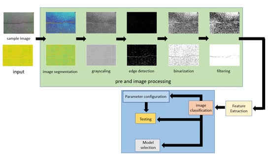
3. Methodology
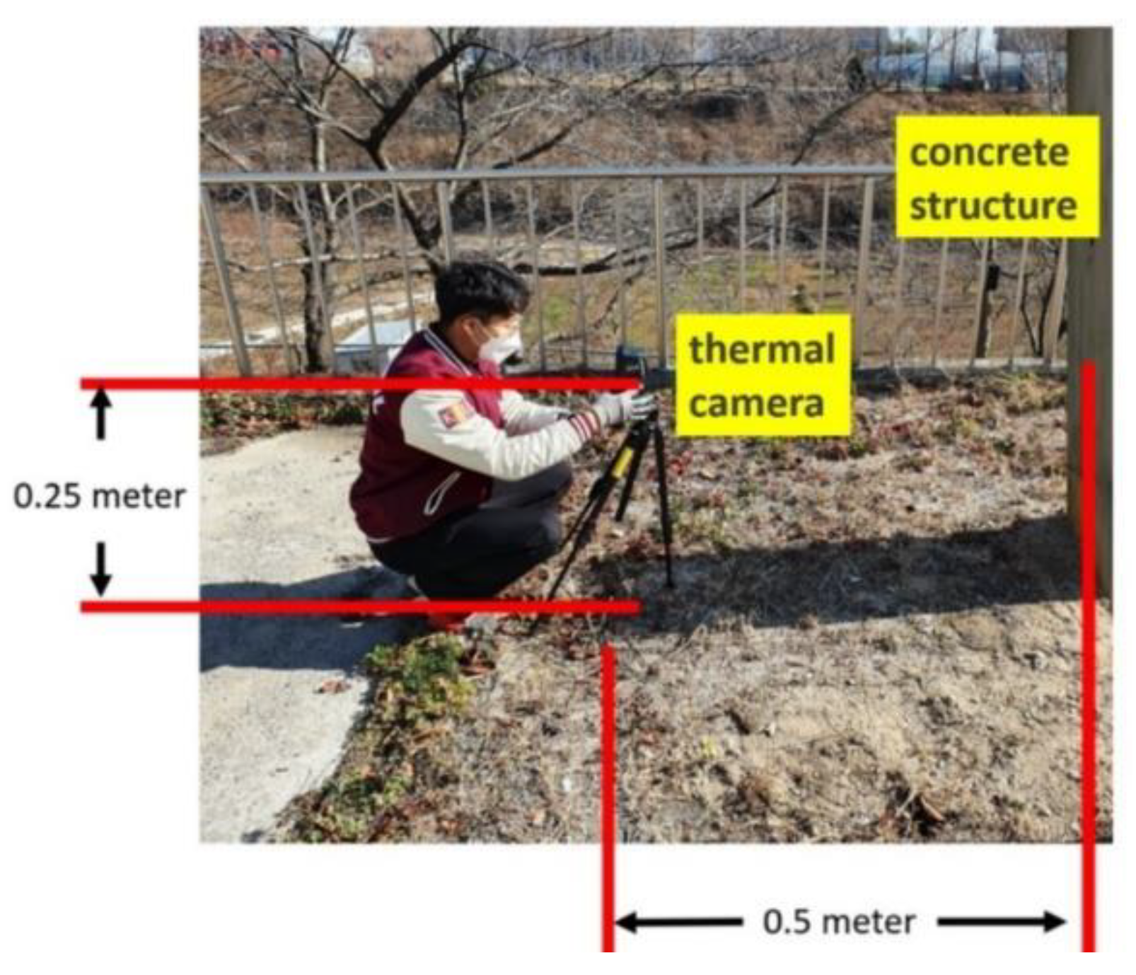
3.1. Image Acquisition
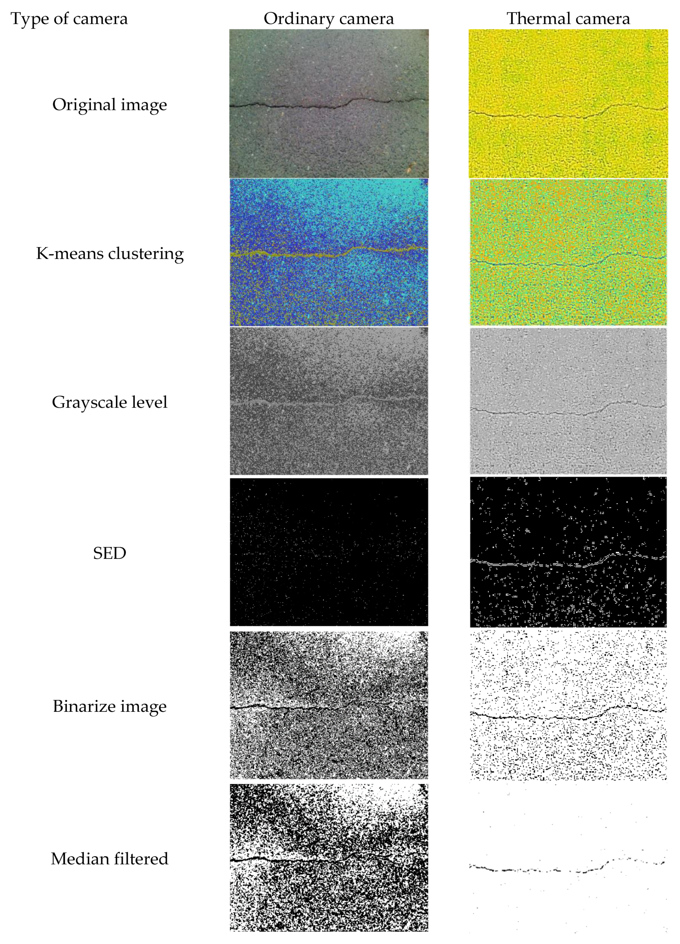
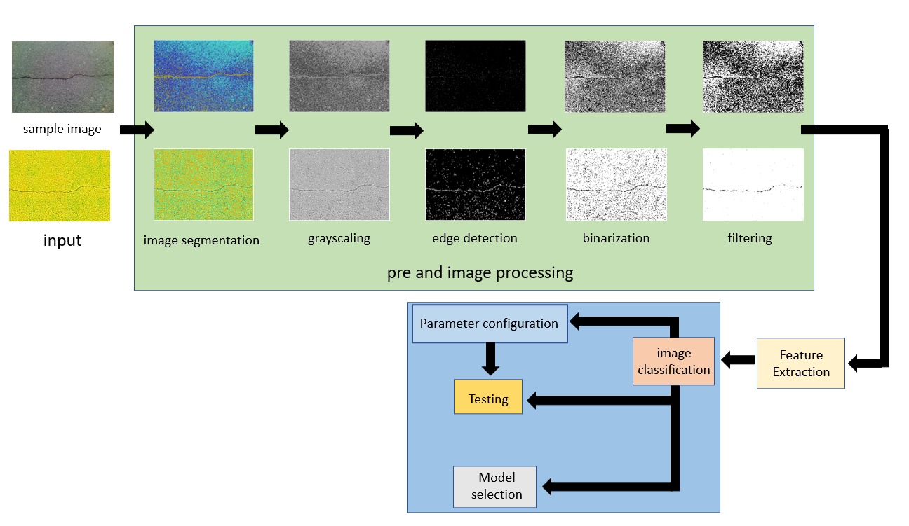
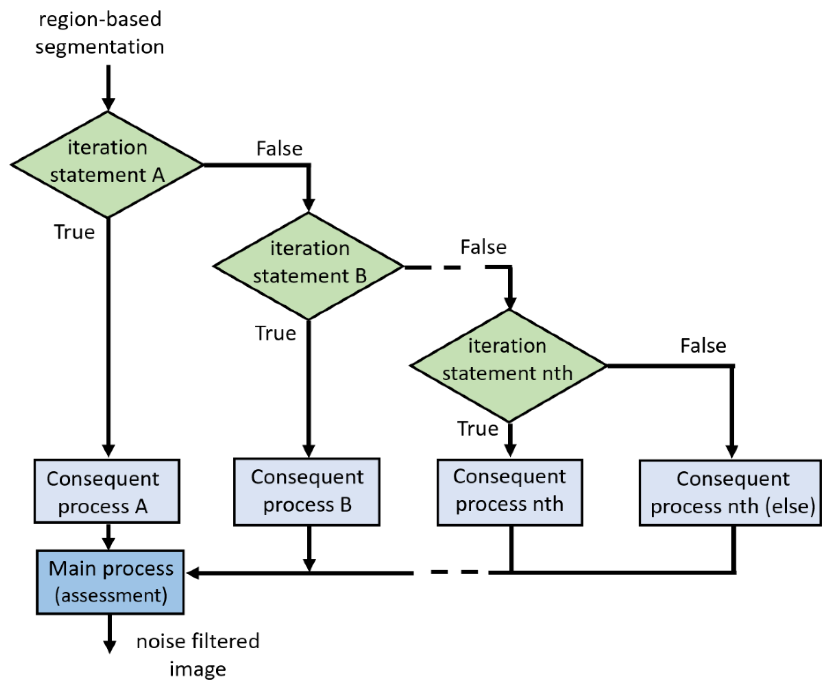
3.2. Algorithm
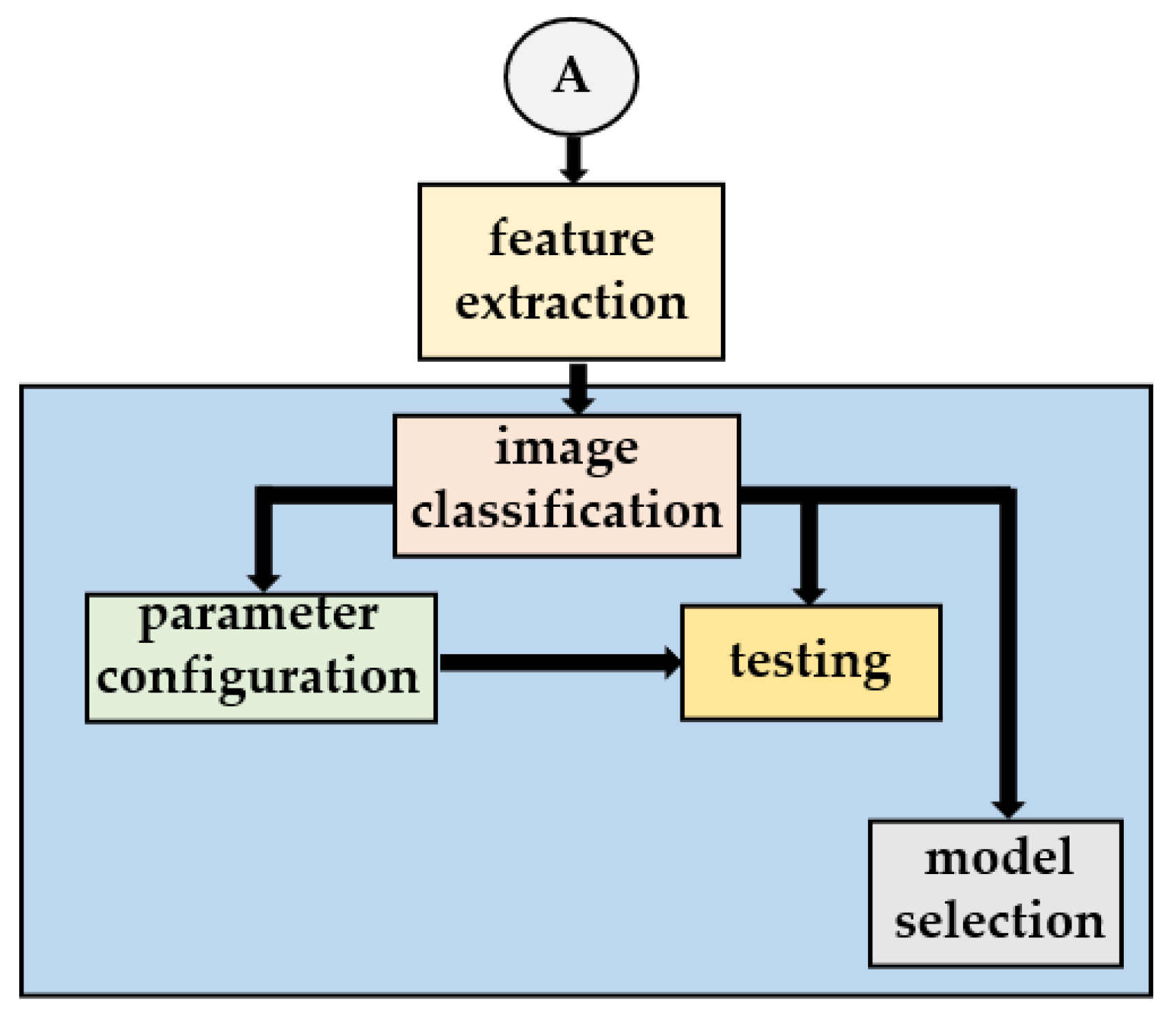
3.3. Image Classifier
4. Results and Discussion
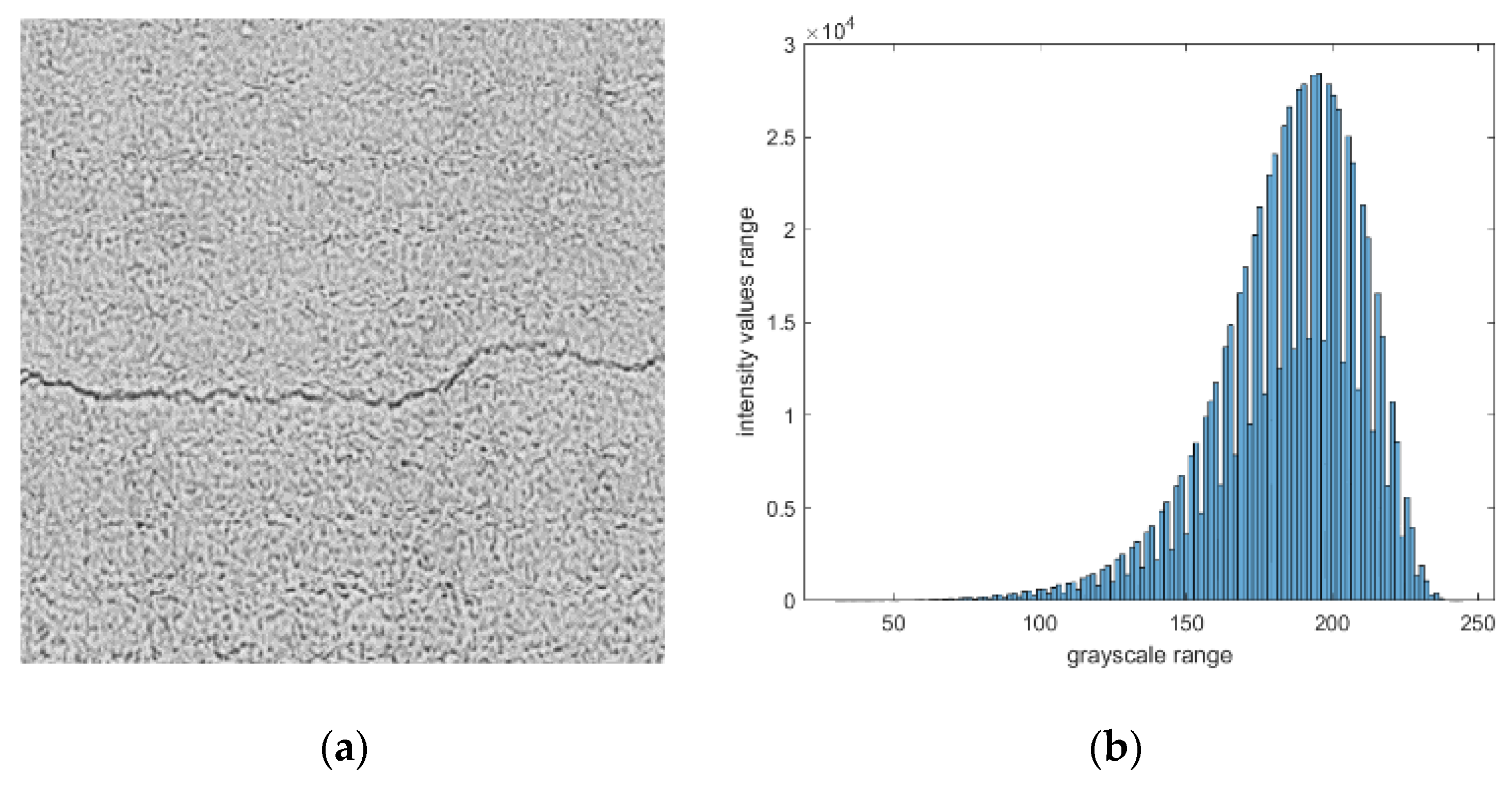
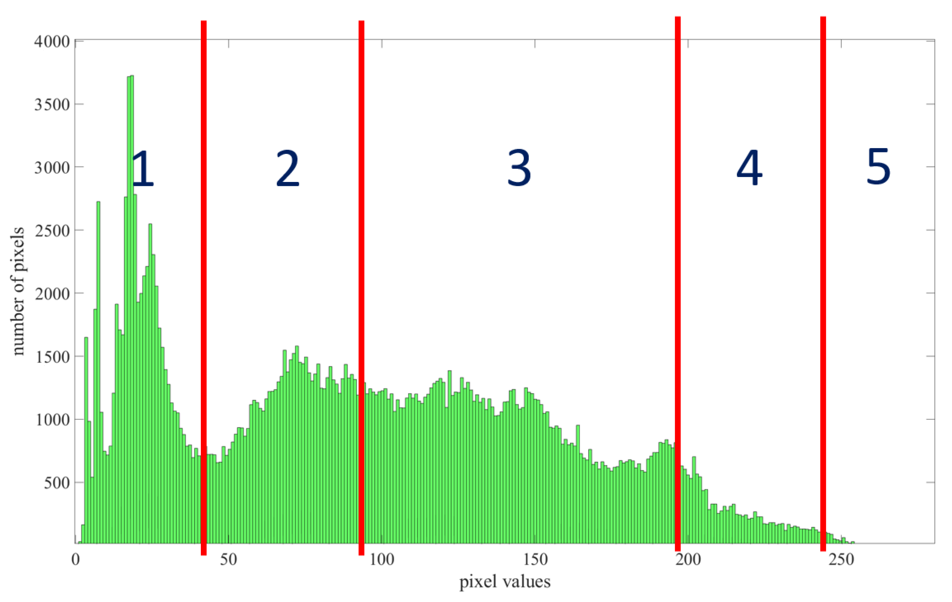
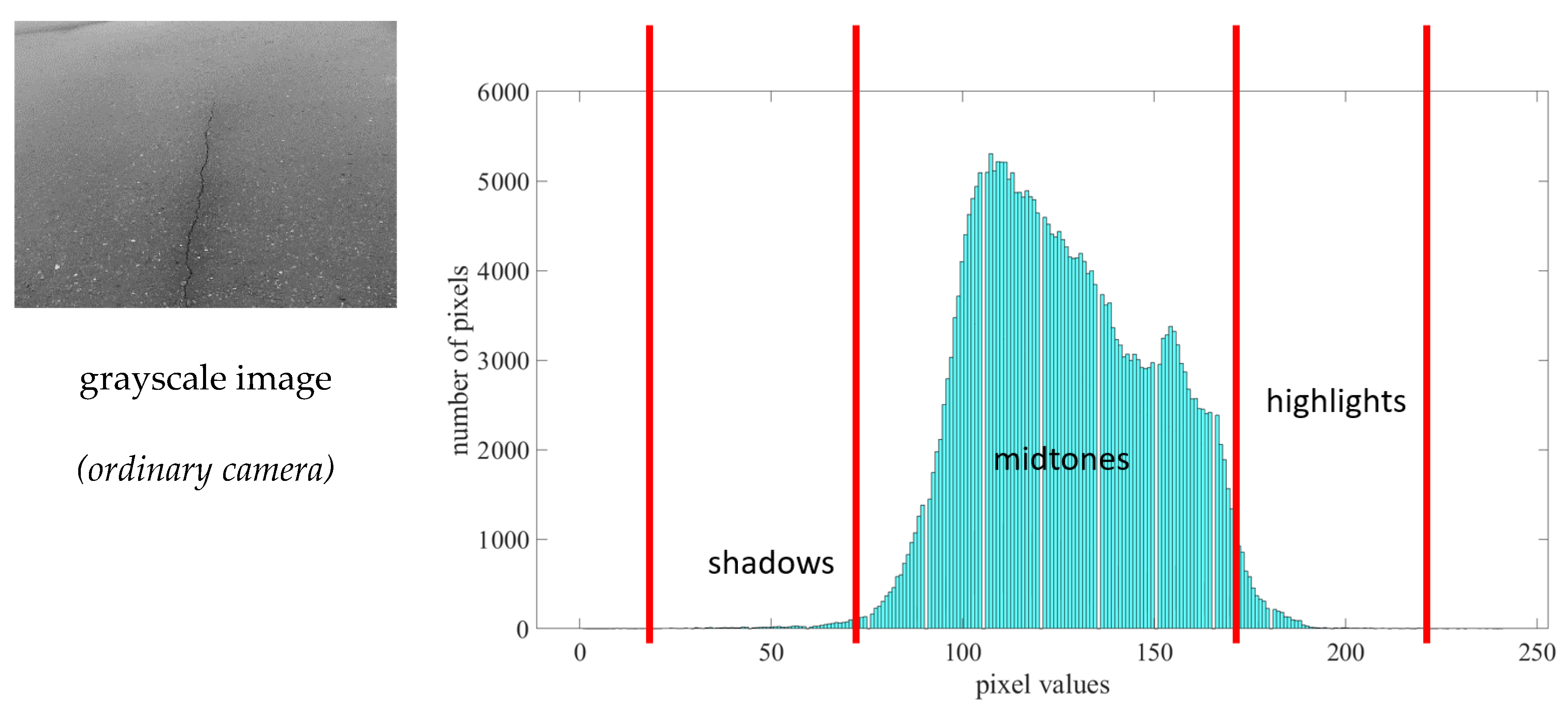
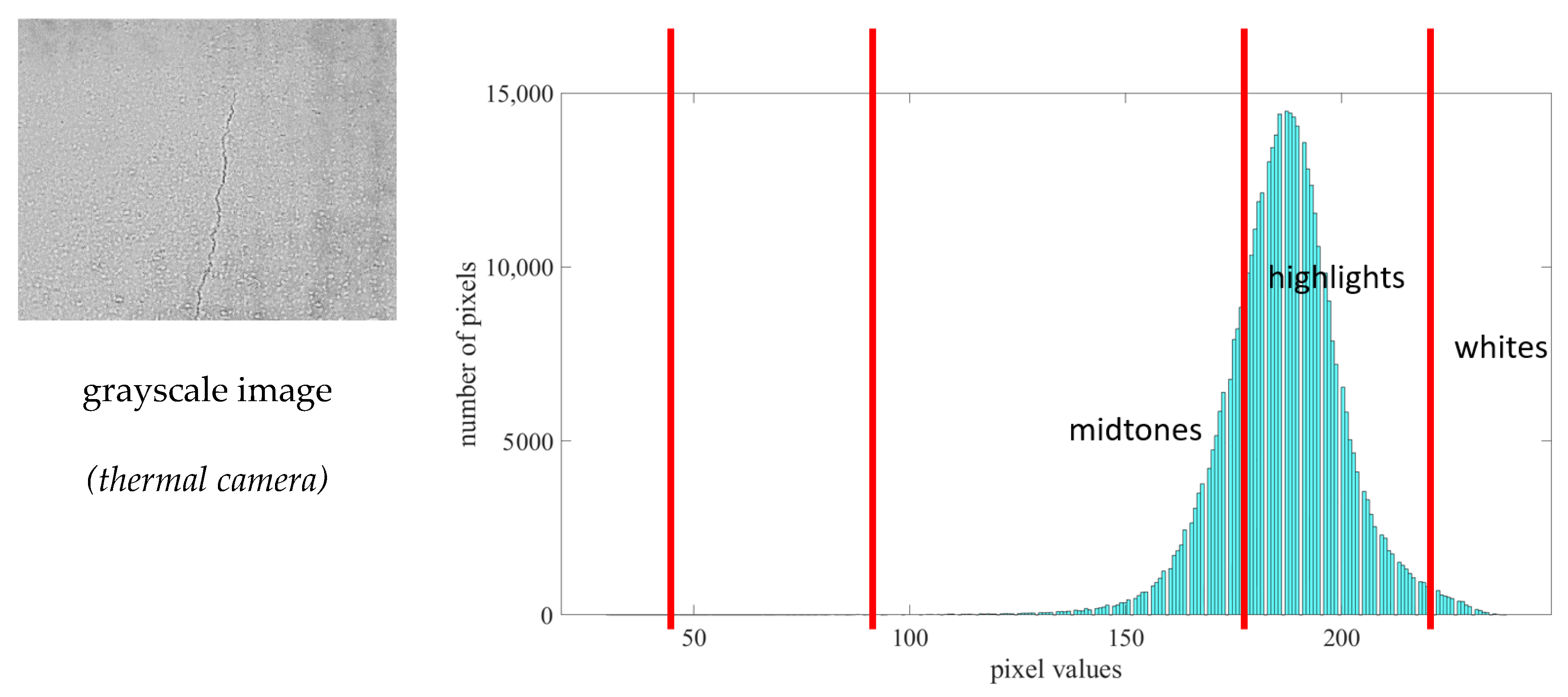
4.1. Analysis of Five Tonal Zone of Histogram
4.2. Image Quality Metrics
5. Conclusions
Author Contributions
Funding
Institutional Review Board Statement
Informed Consent Statement
Data Availability Statement
Conflicts of Interest
Abbreviations
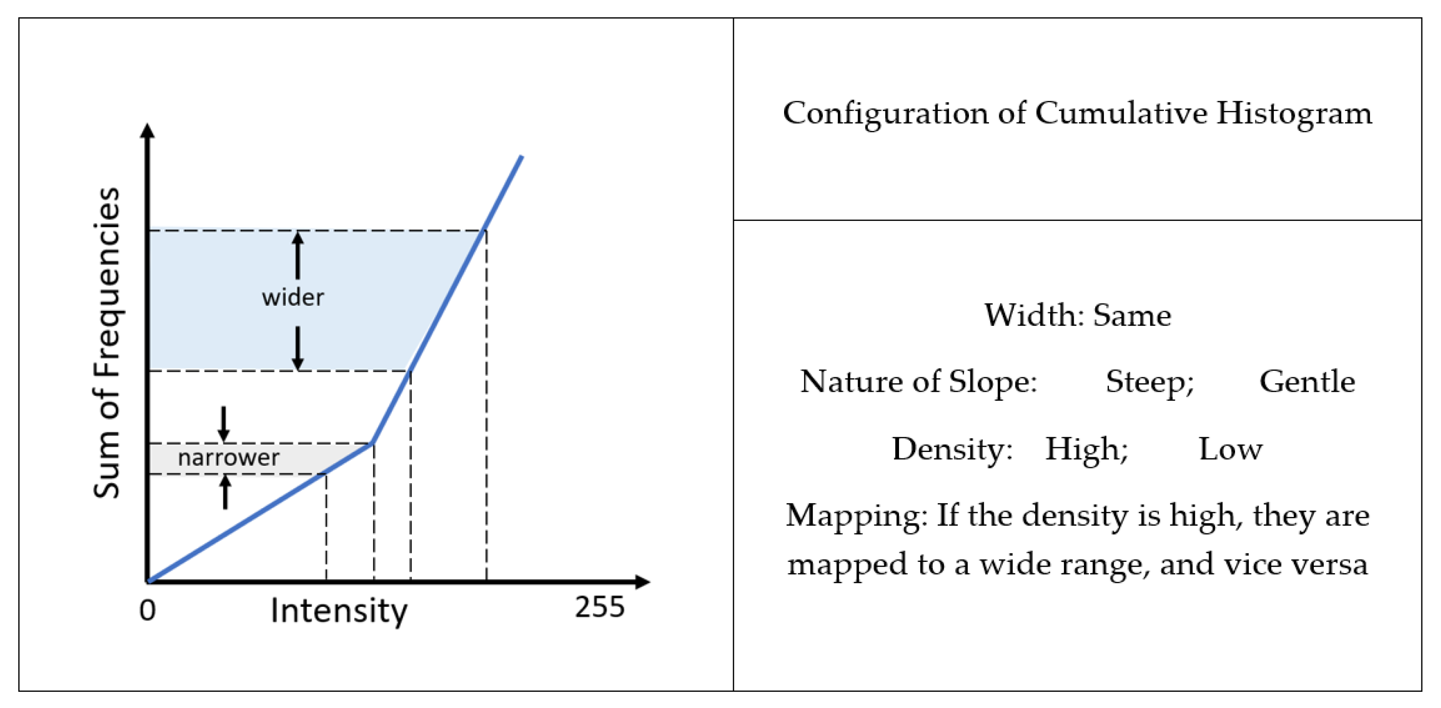
| CDF | Cumulative Distribution Function: this function of image processing presents the resulting image as a linear cumulative distribution function. |
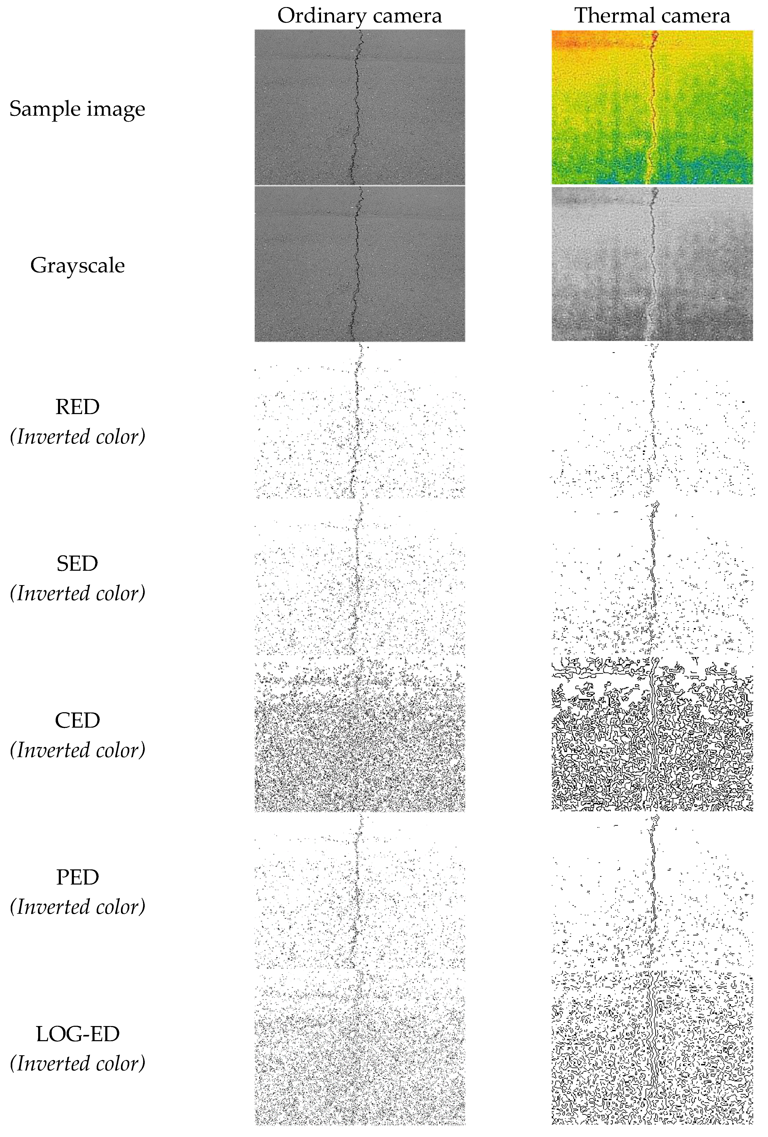
| CED | Canny Edge Detection: this edge detection operator uses a multi-stage algorithm to detect a wide range of edges in images. It locates the intensity gradients of the image and applies non-maximum suppression remove spurious response in the edges. |
| CNN | Convolutional Neural Network: this provides the function of classification of images. |
| ED | Edge Detection: this technique identifies points in a digital image with discontinuities. It sharpens changes in the image brightness. |
| FN | False Negative: this provides the predicted “no”, indicating that non-defective concrete images are classified as “defective”. |
| FP | False Positive: this provides the predicted “yes”, indicating that cracked images are classified inaccurately as “non-defective”. |
| HE | Histogram Equalization: this function is a method in digital image processing that provides contrast adjustment using the histogram of the sampled image. |
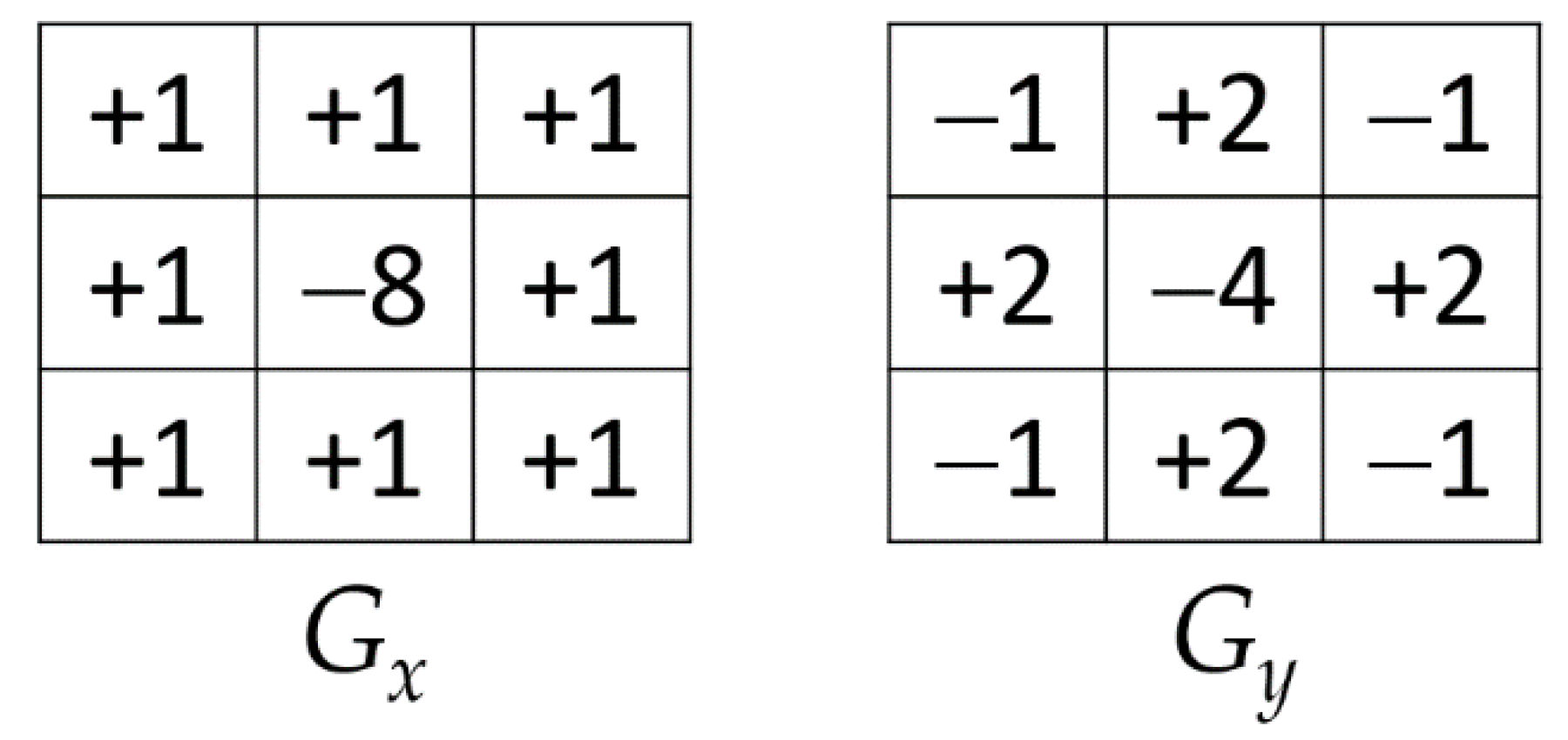
| LOG-ED | Laplacian of Gaussian Edge Detection: initially, this smoothens an image, and it then calculates the Laplacian. The process results in a double-edged image. It finds edges and then locates the zero-crossing between the double edges. |
| ML | Machine Learning: this simply predicts outcomes of classifying the sampled images. Machine learning algorithms use historical data as input to predict new output values. |
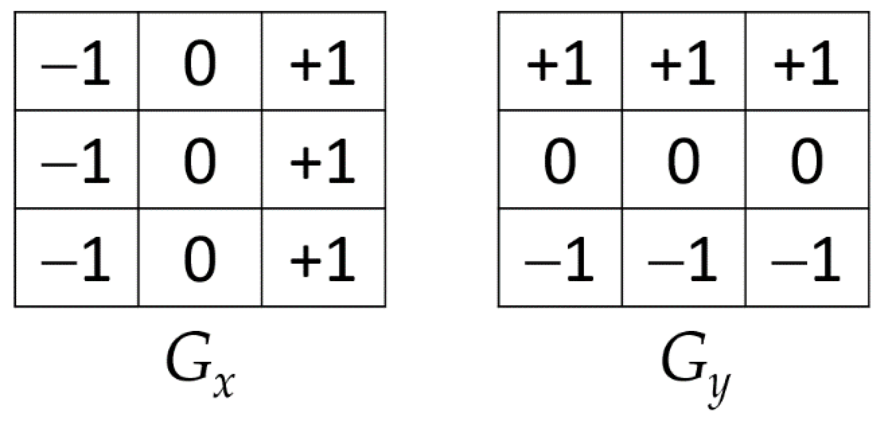
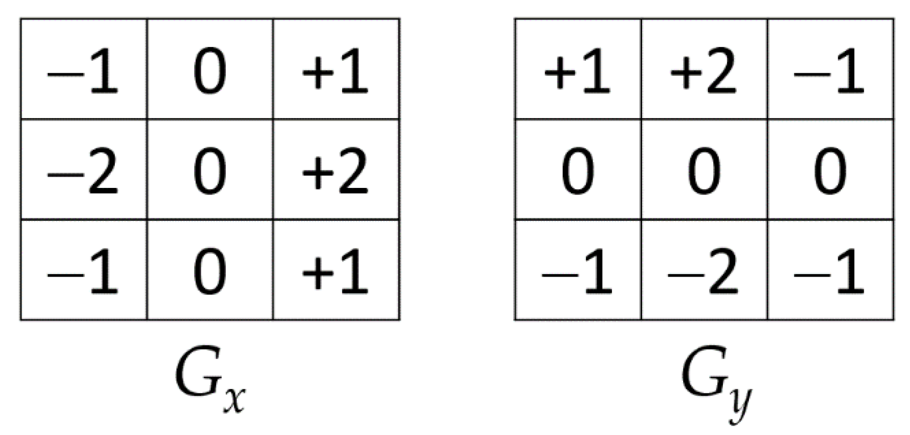
| PED | Prewitt Edge Detection: this operator is appropriate for detecting the magnitude and orientation of edges. It also has the same parameters as Sobel edge detection; however, it is easier to implement. |
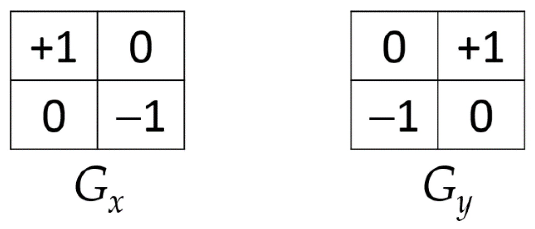
| RED | Robert’s Edge Detection: this operator is a straightforward and efficient approach to quantifying an image’s spatial gradient. The pixel value at a location in the produced image represents the estimated absolute magnitude value of the inputted image’s spatial gradient at that location. |
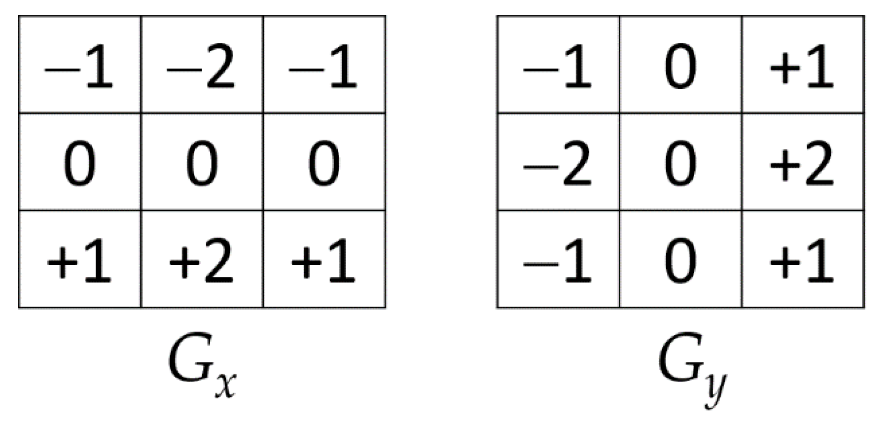
| SED | Sobel Edge Detection: this operator works by calculating the gradient of the intensity of the digital image at each pixel within the image. It locates the direction of the maximum increase from light to dark and the rate of change in that direction. |
| SNR | Signal-to-Noise Ratio: this function is a general metric for determining image quality. It is described as the relative strength of an aimed signal from a sample compared with the undesired background signal from noise. |
| TN | True Negative: this provides the predicted “no”, indicating that cracked images are classified correctly as “defective”. |
| TP | True Positive: this provides the predicted “yes”, indicating that non-defective concrete images are classified correctly as “non-defective”. |
Appendix A. Fundamental Definitions of Terms Used in This Article
Appendix A.1. Image-Processing Analysis
Appendix A.1.1. Fundamentals of Image Parameters
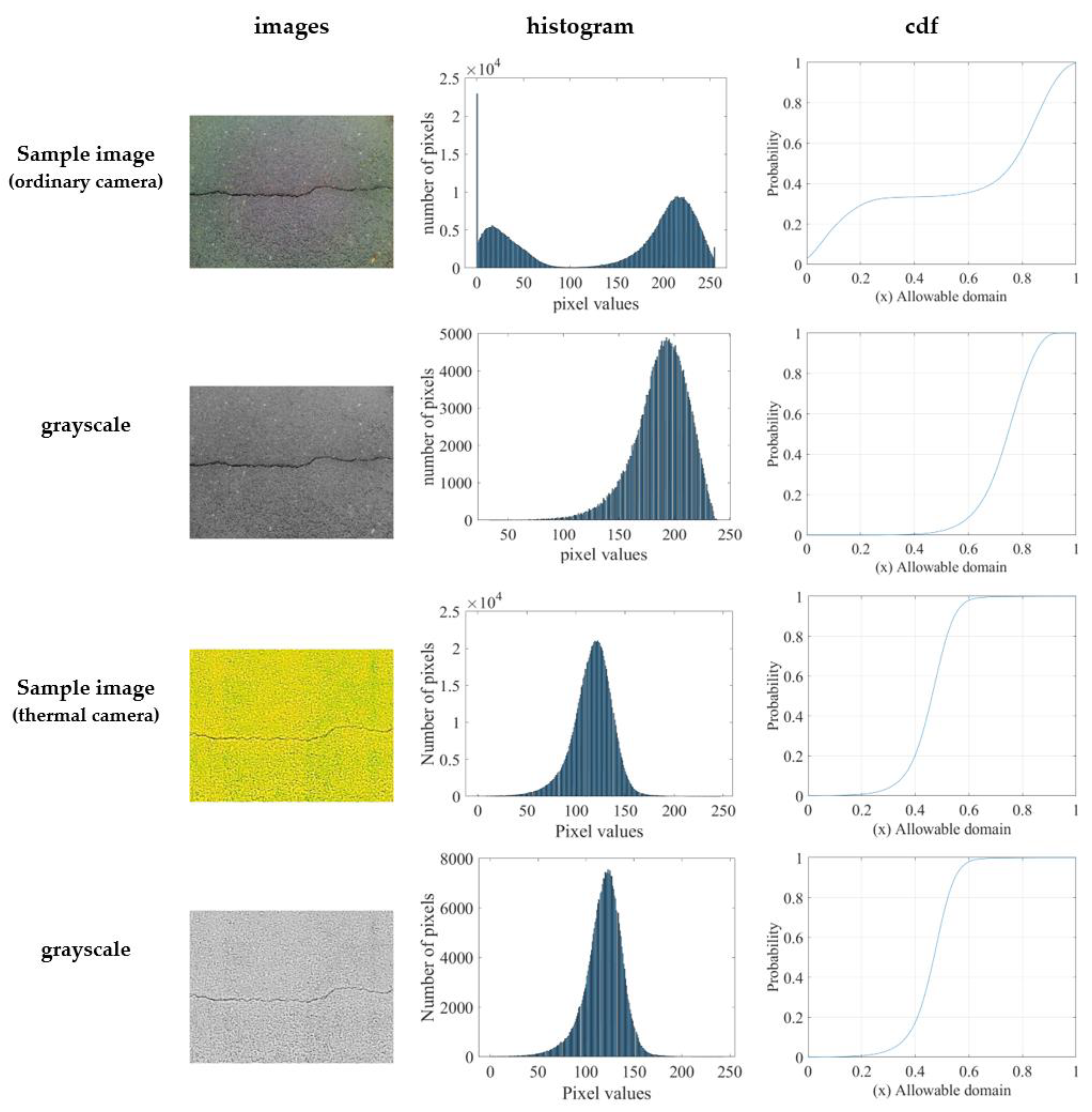
Appendix A.1.2. Graphical Representation of Digital Image
Histogram
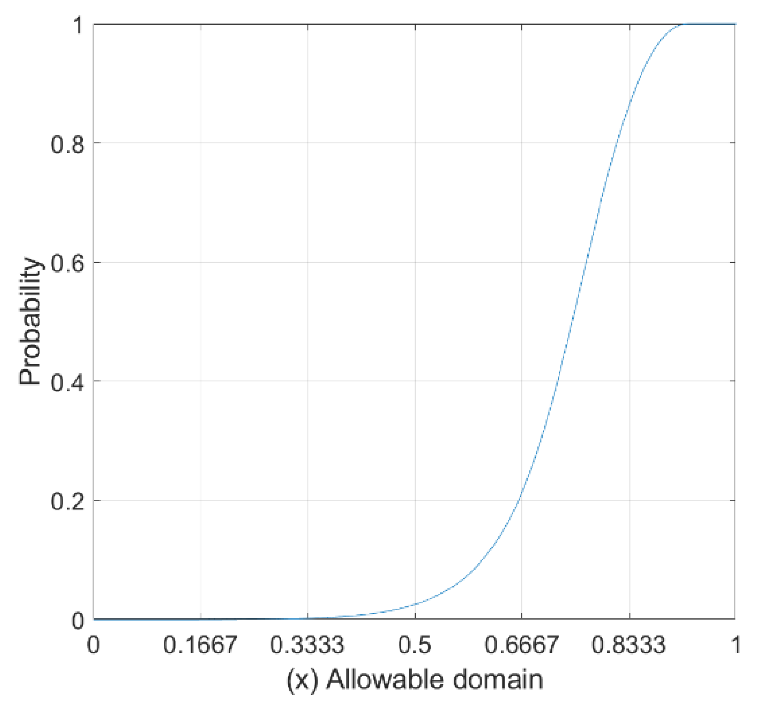
CDF

Appendix A.1.3. Factors That Affect Image Quality
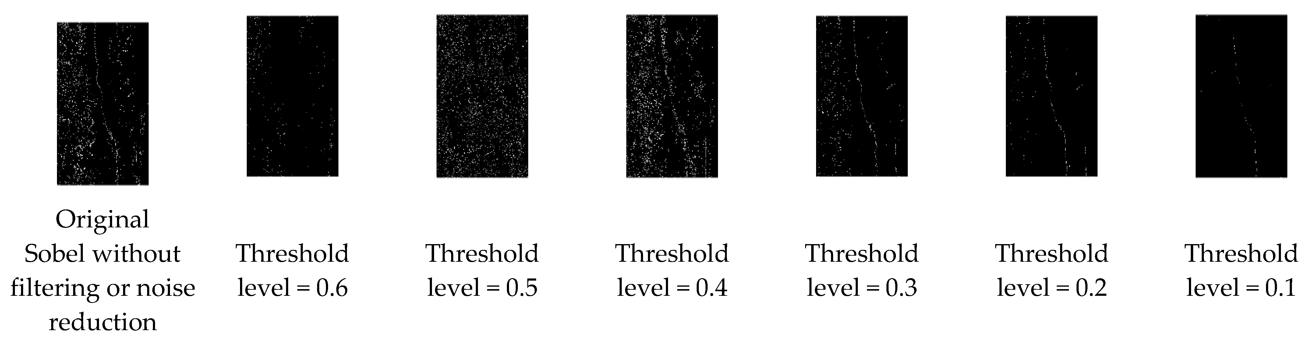
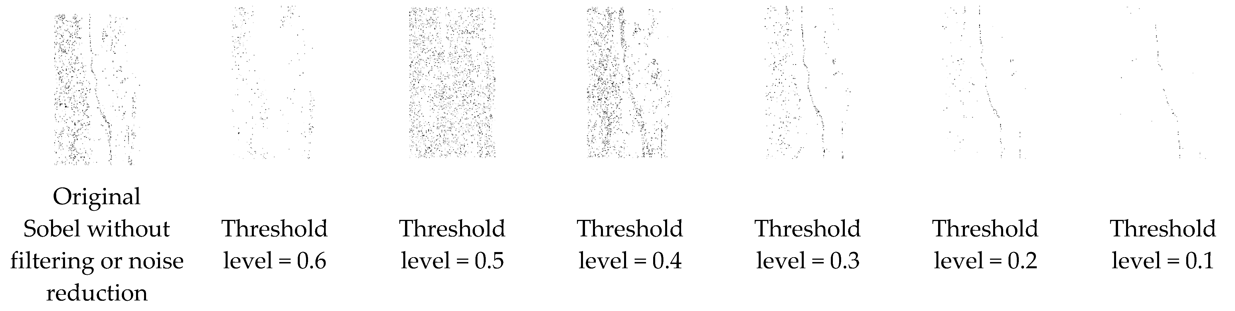
Appendix A.1.4. Image ED Methods for Image Segmentation
Image Segmentation
ED Techniques

References
- Kim, B.; Yuvaraj, N.; Preethaa, K.S.; Hu, G.; Lee, D.-E. Wind-Induced Pressure Prediction on Tall Buildings Using Generative Adversarial Imputation Network. Sensors 2021, 21, 2515. [Google Scholar] [CrossRef] [PubMed]
- Hüthwohl, P.; Brilakis, I. Detecting healthy concrete surfaces. Adv. Eng. Inform. 2018, 37, 150–162. [Google Scholar] [CrossRef]
- Liu, Y.; Yeoh, J.K.W.; Chua, D.K.H. Deep Learning–Based Enhancement of Motion Blurred UAV Concrete Crack Images. J. Comput. Civ. Eng. 2020, 34, 04020028. [Google Scholar] [CrossRef]
- Kim, B.; Yuvaraj, N.; Tse, K.T.; Lee, D.E.; Hu, G. Pressure pattern recognition in buildings using an unsupervised machine-learning algorithm. J. Wind. Eng. Ind. Aerodyn. 2021, 214, 1–18. [Google Scholar] [CrossRef]
- Chen, Z.; Kim, B.; Lee, D.E. Aerodynamic characteristics and lateral displacements of a set of two buildings in a linked tall building system. Sensors 2021, 21, 4046. [Google Scholar] [CrossRef] [PubMed]
- Bhosale, A.B.; Lakavath, C.; Prakash, S.S. Multi-linear tensile stress-crack width relationship s for hybrid fibre reinforced concrete using inverse analysis and digital image correlation. Eng. Struct. 2020, 225, 1–19. [Google Scholar] [CrossRef]
- Zhu, Z.; Brilakis, I. Parameter optimization for automated concrete detection in image data. Autom. Constr. 2010, 19, 944–953. [Google Scholar] [CrossRef]
- Yeh, P.; Liu, P. Imaging of internal cracks in concrete structures using the surface rendering technique. NDT E Int. 2009, 42, 181–187. [Google Scholar] [CrossRef]
- Omar, T.; Nehdi, M. Remote sensing of concrete bridge decks using unmanned aerial vehicle infrared thermography. Autom. Constr. 2017, 83, 360–371. [Google Scholar] [CrossRef]
- Dogan, G.; Arslan, M.H.; Ceylan, M. Concrete compressive strength detection using image processing based new test method. Measurement 2017, 109, 137–148. [Google Scholar] [CrossRef]
- Bhattacharya, G.; Mandal, B.; Puhan, N.B. Multi-deformation aware attention learning for concrete structural defect classification. IEEE Trans. Circuits Syst. Video 2020, 31, 3707–3713. [Google Scholar] [CrossRef]
- Başyiğit, C.; Çomak, B.; Kılınçarslan, Ş.; Üncü, İ.S. Assessment of concrete compressive strength by image processing technique. Constr. Build. Mater. 2012, 37, 526–532. [Google Scholar] [CrossRef]
- Fang, F.; Li, L.; Gu, Y.; Zhu, H.; Lim, J.-H. A novel hybrid approach for crack detection. Pattern Recognit. 2020, 107, 107474. [Google Scholar] [CrossRef]
- Kabir, S. Imaging-based detection of AAR induced map-cracking damage in concrete structure. NDT E Int. 2010, 43, 461–469. [Google Scholar] [CrossRef]
- Kong, S.Y.; Fan, J.S.; Liu, Y.F.; Wei, X.C.; Ma, X.W. Automated crack assessment and quantitative growth monitoring. Comput. Aided Civ. Infrastruct. Eng. 2020, 36, 656–674. [Google Scholar] [CrossRef]
- Chow, J.K.; Su, Z.; Wu, J.; Li, Z.; Tan, P.S.; Liu, K.; Mao, X.; Wang, Y.H. Artificial intelligence-empowered pipeline for image-based inspection of concrete structures. Autom. Constr. 2020, 120, 103372. [Google Scholar] [CrossRef]
- Hsieh, Y.A.; Tsai, Y.J. Machine learning for crack detection: Review and model performance comparison. J. Comput. Civ. Eng. 2020, 34, 1–12. [Google Scholar] [CrossRef]
- Ma, J.; Song, W.-G.; Fang, Z.-M.; Lo, S.-M.; Liao, G.-X. Experimental study on microscopic moving characteristics of pedestrians in built corridor based on digital image processing. Build. Environ. 2010, 45, 2160–2169. [Google Scholar] [CrossRef]
- Zhang, Q.; An, Z.; Liu, T.; Zhang, Z.; Huangfu, Z.; Li, Q.; Yang, Q.; Liu, J. Intelligent rolling compaction system for earth-rock dams. Autom. Constr. 2020, 116, 103246. [Google Scholar] [CrossRef]
- Song, Y.; Huang, Z.; Shen, C.; Shi, H.; Lange, D.A. Deep learning-based automated image segmentation for concrete petrographic analysis. Cem. Concr. Res. 2020, 135, 106118. [Google Scholar] [CrossRef]
- Jung, H.K.; Park, G. Rapid and non-invasive surface crack detection for pressed-panel products based on online image processing. Struct. Health Monit. 2018, 18, 1928–1942. [Google Scholar] [CrossRef]
- Talab, A.M.A.; Huang, Z.; Xi, F.; HaiMing, L. Detection crack in image using Otsu method and multiple filtering in image processing techniques. Optik 2016, 127, 1030–1033. [Google Scholar] [CrossRef]
- Abdel-Qader, I.; Abudayyeh, O.; Kelly, M.E. Analysis of Edge-Detection Techniques for Crack Identification in Bridges. J. Comput. Civ. Eng. 2003, 17, 255–263. [Google Scholar] [CrossRef]
- Dorafshan, S.; Thomas, R.J.; Maguire, M. Comparison of deep convolutional neural networks and edge detectors for image-based crack detection in concrete. Constr. Build. Mater. 2018, 186, 1031–1045. [Google Scholar] [CrossRef]
- Tong, Z.; Gao, J.; Zhang, H. Recognition, location, measurement, and 3D reconstruction of concealed cracks using convolutional neural networks. Constr. Build. Mater. 2017, 146, 775–787. [Google Scholar] [CrossRef]
- Kim, B.; Yuvaraj, N.; Preethaa, K.R.S.; Pandian, R.A. Surface crack detection using deep learning with shallow CNN architecture for enhanced computation. Neural Comput. Appl. 2021, 33, 9289–9305. [Google Scholar] [CrossRef]
- Kim, B.; Yuvaraj, N.; Preethaa, K.R.S.; Santhosh, R.; Sabari, A. Enhanced pedestrian detection using optimized deep convolution neural network for smart building surveillance. Soft Comput. 2020, 24, 17081–17092. [Google Scholar] [CrossRef]
- Kim, B.; Serfa Juan, R.O.; Lee, D.-E.; Chen, Z. Importance of Image Enhancement and CDF for Fault Assessment of Photovoltaic Module Using IR Thermal Image. Appl. Sci. 2021, 11, 8388. [Google Scholar] [CrossRef]
- Shamsolmoali, P.; Zareapoor, M.; Zhang, J.; Yang, J. Image super resolution by dilated dense progressive network. Image Vis. Comput. 2019, 88, 9–18. [Google Scholar] [CrossRef]
- Chan, F.K.S.; Kong, A.W.K. A further study of low resolution androgenic hair patterns as a soft biometric trait. Image Vis. Comput. 2018, 69, 125–142. [Google Scholar] [CrossRef]
- Elliott, M.A.; Insko, E.K.; Greenman, R.L.; Leigh, J.S. Improved Resolution and Signal-to-Noise Ratio in MRI via Enhanced Signal Digitization. J. Magn. Reson. 1998, 130, 300–304. [Google Scholar] [CrossRef]
- Zelelew, H.M.; Papagiannakis, A.T. A volumetrics thresholding algorithm for processing asphalt concrete X-ray CT images. Int. J. Pavement Eng. 2011, 12, 543–551. [Google Scholar] [CrossRef]
- Pardo, A.; Sapiro, G. Visualization of high dynamic range images. IEEE Trans. Image Process. 2003, 12, 639–647. [Google Scholar] [CrossRef] [PubMed] [Green Version]
- Yu, S.; Dai, G.; Wang, Z.; Li, L.; Wei, X.; Xie, Y. A consistency evaluation of signal-to-noise ratio in the quality assessment of human brain magnetic resonance images. BMC Med. Imaging 2018, 18, 17. [Google Scholar] [CrossRef] [Green Version]
- Khormani, M.; Jaari, V.R.K.; Aghayan, I.; Ghaderi, S.H.; Ahmadyfard, A. Compressive strength determination of concrete specimens using X-ray computed tomography and finite element method. Constr. Build. Mater. 2020, 256, 119427. [Google Scholar] [CrossRef]
- Jasmine, J.; Annadurai, S. Real time video image enhancement approach using particle swarm optimisation technique with adaptive cumulative distribution function based histogram equalization. Measurement 2019, 145, 833–840. [Google Scholar] [CrossRef]
- Gao, X.; Lu, W.; Tao, D.; Li, X. Image Quality Assessment Based on Multiscale Geometric Analysis. IEEE Trans. Image Process. 2009, 18, 1409–1423. [Google Scholar]
- Kabir, S.; Rivard, P.; He, D.-C.; Thivierge, P. Damage assessment for concrete structure using image processing techniques on acoustic borehole imagery. Constr. Build. Mater. 2009, 23, 3166–3174. [Google Scholar] [CrossRef]
- Bugarinović, Ž.; Pajewski, L.; Ristić, A.; Vrtunski, M.; Govedarica, M.; Borisov, M. On the introduction of canny operator in an advanced imaging algorithm for real-time detection of hyperbolas in ground-penetrating radar data. Electronics 2020, 9, 541. [Google Scholar] [CrossRef] [Green Version]


| Brand/Company Name | FLIR E8 |
|---|---|
| Field of View | 45° × 34° |
| Object Temperature Range | −20 °C to 250 °C |
| Image Frequency | 9 Hz |
| Thermal Sensitivity | <0.06 °C |
| Accuracy | ±2 °C |
| Thermal Palettes | Iron, Rainbow, Grayscale |
| File Format | Radiometric JPG |
| On-board Digital Camera | 640 × 480 |
| Ordinary Camera | Thermal Camera | |
|---|---|---|
| images |  |  |
| MSE | 23,432.0312 | 240.7319 |
| PSNR | 4.4327 | 24.3155 |
| SNR | 4.4053 | 24.2881 |
| MS-SSIM | 0.0321 | 0.7885 |
| BRISQUE | 43.4582 | 45.0100 |
| NIQE | 15.1913 | 13.2069 |
| PIQE | 63.0411 | 88.7166 |
| Classifier Method | Percent Sensitivity | Percent Specificity | Percent Accuracy |
|---|---|---|---|
| CNN | 98% | 94.96 | 93.96 |
| CNN-SVM | 99% | 95.3% | 98% |
| Classifier Method | Percent Sensitivity | Percent Specificity | Percent Accuracy |
|---|---|---|---|
| CNN | 94.25 | 90% | 90% |
| CNN-SVM | 97.55% | 93.65% | 93.96% |
| Coefficient | CNN | CNN–SVM |
|---|---|---|
| Correlation | 0.9321 | 0.9981 |
| Regression | 0.9629 | 0.9995 |
Publisher’s Note: MDPI stays neutral with regard to jurisdictional claims in published maps and institutional affiliations. |
© 2021 by the authors. Licensee MDPI, Basel, Switzerland. This article is an open access article distributed under the terms and conditions of the Creative Commons Attribution (CC BY) license (https://creativecommons.org/licenses/by/4.0/).
Share and Cite
Kim, B.; Choi, S.-W.; Hu, G.; Lee, D.-E.; Serfa Juan, R.O. Multivariate Analysis of Concrete Image Using Thermography and Edge Detection. Sensors 2021, 21, 7396. https://doi.org/10.3390/s21217396
Kim B, Choi S-W, Hu G, Lee D-E, Serfa Juan RO. Multivariate Analysis of Concrete Image Using Thermography and Edge Detection. Sensors. 2021; 21(21):7396. https://doi.org/10.3390/s21217396
Chicago/Turabian StyleKim, Bubryur, Se-Woon Choi, Gang Hu, Dong-Eun Lee, and Ronnie O. Serfa Juan. 2021. "Multivariate Analysis of Concrete Image Using Thermography and Edge Detection" Sensors 21, no. 21: 7396. https://doi.org/10.3390/s21217396
APA StyleKim, B., Choi, S.-W., Hu, G., Lee, D.-E., & Serfa Juan, R. O. (2021). Multivariate Analysis of Concrete Image Using Thermography and Edge Detection. Sensors, 21(21), 7396. https://doi.org/10.3390/s21217396