
Fault Detection in the MSW Incineration Process Using Stochastic Configuration Networks and Case-Based Reasoning

Abstract
:1. Introduction
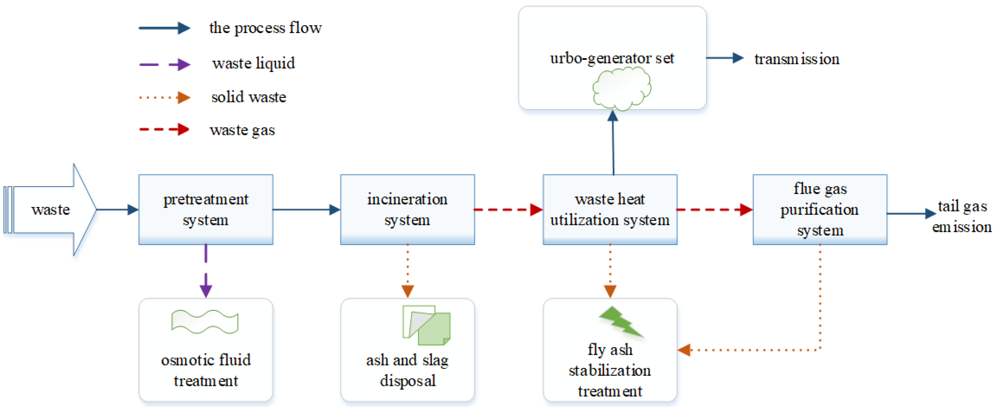
2. Fault Description of MSW Incineration Process
3. Fault Detection Model for MSW Incineration Process
3.1. SCN-LPM Method
- (1)
- Constructing sample set. Ck is a subset of sample set C that represents some kinds of real data. M is an n-dimensional extractor that can map Ck to its characteristic space Fk. Namely:where x is an element in a point set . Sample set D is defined as follows:where × represents Cartesian product, which can be obtained by combining any two characteristic attributes Fi and Fj. represents the Dirichlet symbolic function whose value is 0 when x and y belong to the same category; otherwise it is 1. That is, when i = j, δij = 0, otherwise δij = 1. According to the definition of Formula (2), several pairs of sample data can be formed from the sample set and sample set D can be constructed. Sample set D can be divided into training sample set Dtrain and testing sample set Dtest [31], which can be used to train and validate the following network model. The number of sample data pairs formed is p(p − 1)/2.
- (2)
- Training SCN. The SCN model is trained with a training sample set. The selection of SCNs should consider the structure of the network; that is, the number of nodes in the input layer and output layer as well as the number of neurons in the hidden layer are determined. Document [32] describes the determination method, which is described as follows:
3.2. Fault Detection Model Based on SCN-CBR
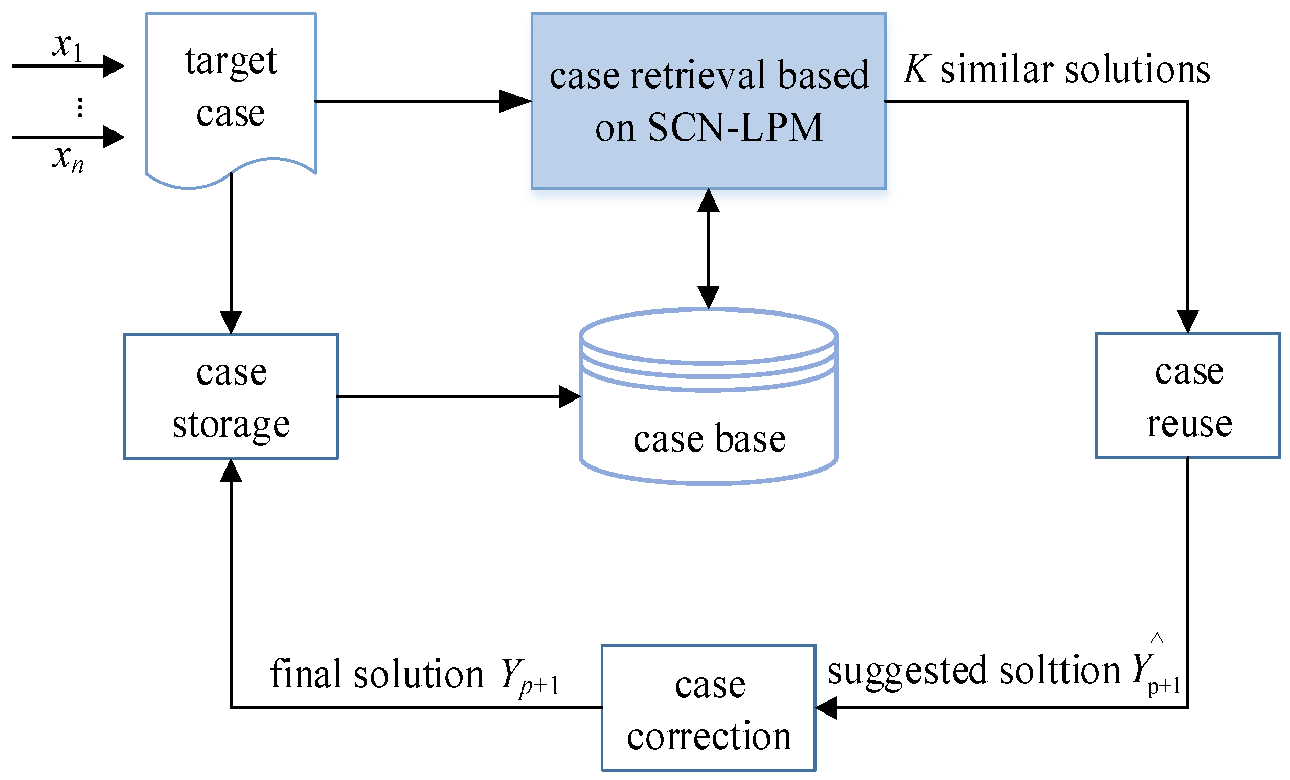
3.2.1. Model Structure and Function
3.2.2. Fault Detection Algorithms
- (1)
- Constructing case base. The problem descriptions and solutions of target case Xp+1 and source case Ck are normalized and expressed as an eigenvector form in binary tuples to form p source cases, which are stored in the case base. Each source case is recorded as . It can be expressed in the form of binary tuples as follows:where p is the total number of source cases, Xk is the set of characteristic attributes in the k-th source cases, and Yk is the category of characteristic attributes in the k-th source cases. Assuming that each source case has n characteristic attributes, Xk can be expressed in the following form:where xi,k is the normalized value of the i-th characteristic attribute in the record of article k-th.
- (2)
- Case retrieval based on SCN-LPM. The input variable of the target case Xp+1 and the input variable of the source case Xk(k = 1, 2, …, p) are composed of p input pairs, namely:Then, p YNN(Xp+1, Xk) can be obtained according to the SCN-LPM method. According to A1 of the four metrics in Section 3.1, K source cases similar to the target case Xp+1 can be obtained.
- (3)
- Case reuse. According to the KNN rule, the number of categories corresponding to the K source cases retrieved is counted, and the category with a large number is taken as the suggested category .
- (4)
- Case revision. When evaluating the suggested category , if the evaluation is unsuccessful, the classification results need to be revised to obtain the correct category .
- (5)
- Case storage. Target case and corrected category are stored in the case base to form a new case. So far, the number of source cases has been from p→p+1, and the CBR problem solving process is completed.
3.3. Algorithmic Steps
4. Experimental Study
4.1. Experimental Parameters
4.2. Performance Testing
4.2.1. Stability
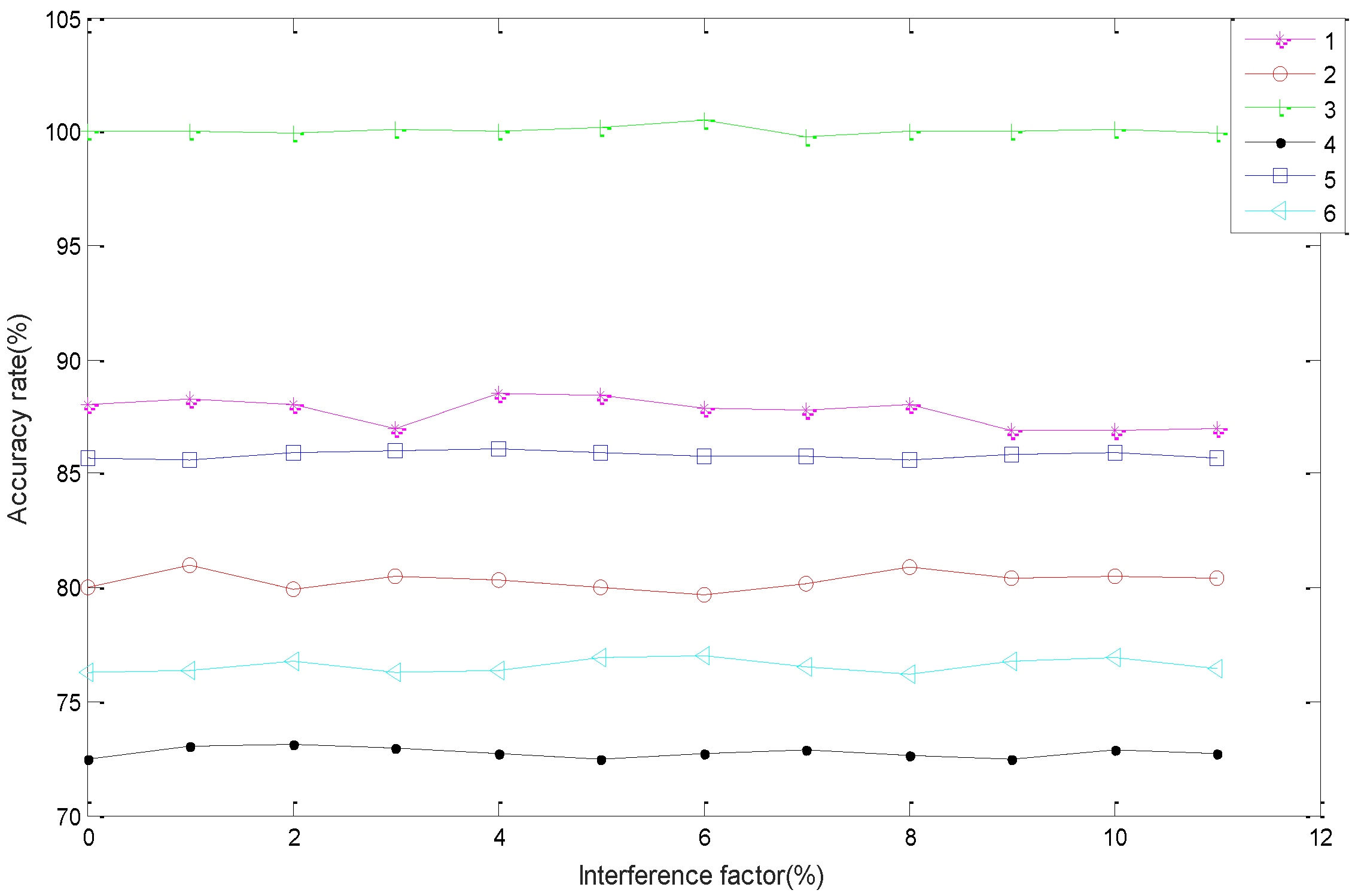
4.2.2. Robustness
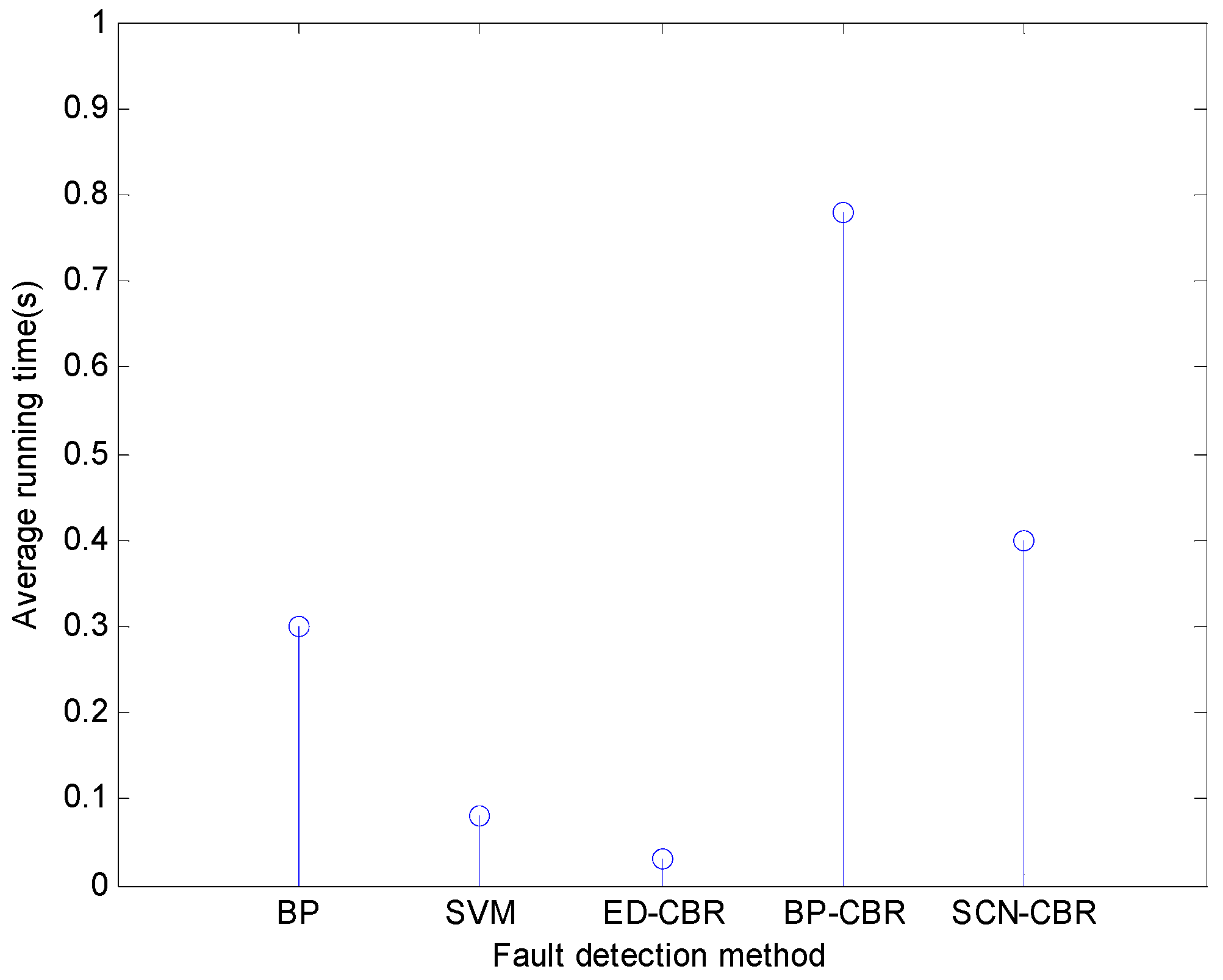
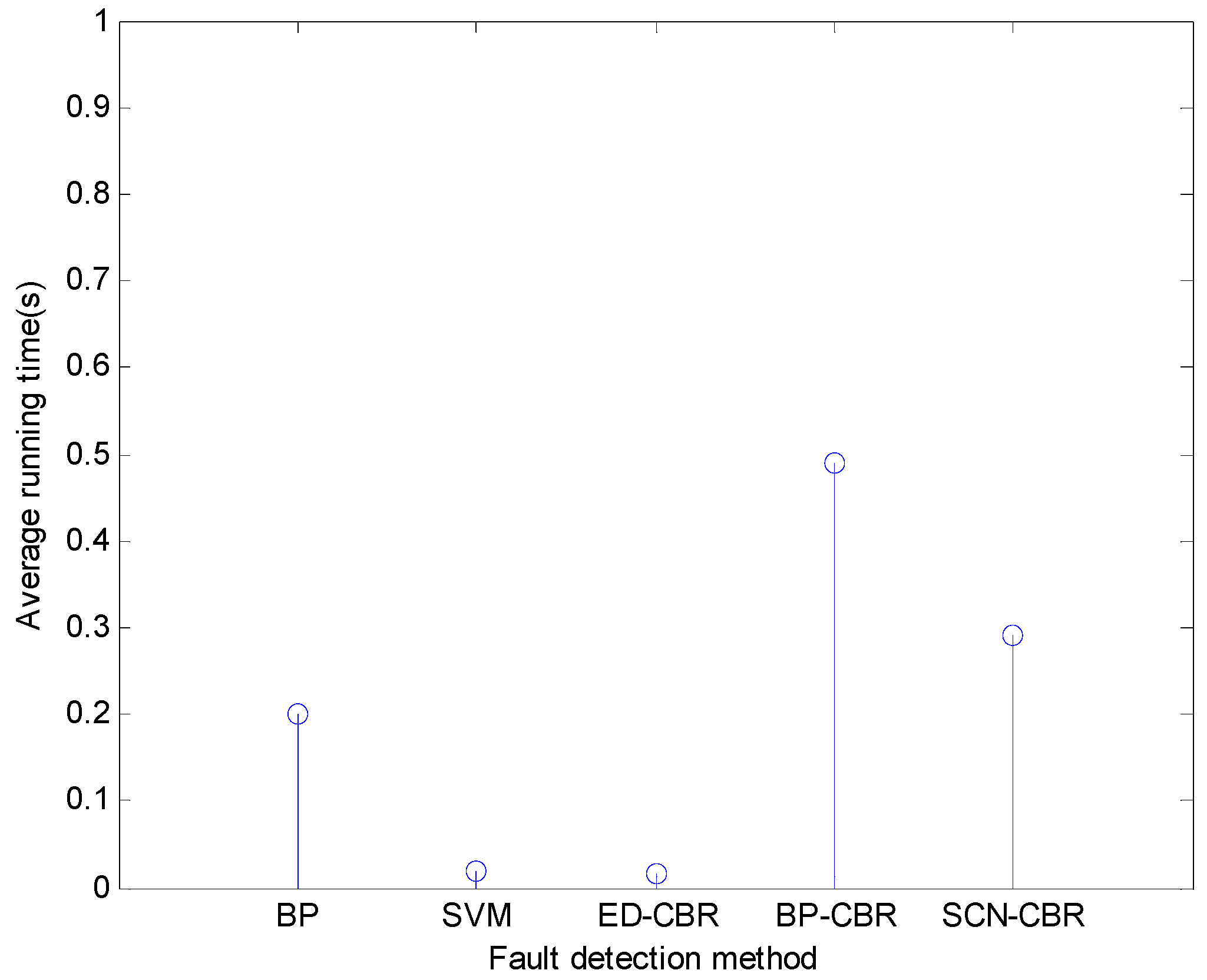
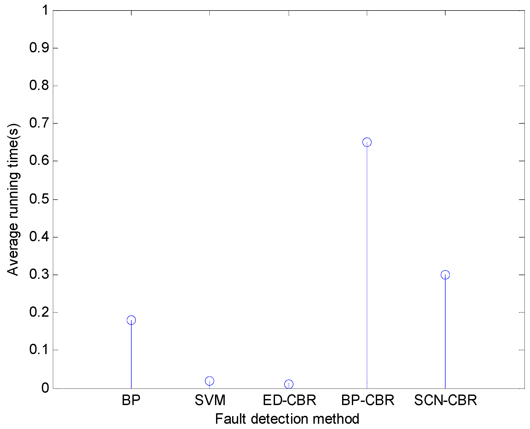
4.3. Contrast Experiments
5. Conclusions
- (1)
- A learning pseudo metric method based on SCN was constructed. First, the sample set was constructed according to the Cartesian product. Then, the pseudo metric criterion was defined. Finally, according to the training sample set and the defined pseudo metric criteria, the SCN learning model was trained, and a new learning pseudo metric method was obtained.
- (2)
- A fault detection model based on SCN-CBR was constructed. The similarity measurement method based on SCN-LPM was applied to the retrieval stage of CBR, and a fault detection model of the waste incineration process based on SCN-CBR was established.
Author Contributions
Funding
Institutional Review Board Statement
Informed Consent Statement
Data Availability Statement
Acknowledgments
Conflicts of Interest
References
- Tozlu, A.; Özahi, E.; Abuşoğlu, A. Waste to energy technologies for municipal solid waste management in Gaziantep. Renew. Sustain. Energy Rev. 2016, 54, 809–815. [Google Scholar] [CrossRef]
- Huang, W. Research on the status quo and supervision countermeasures of urban domestic waste treatment technology. Environ. Dev. 2019, 31, 84–86. [Google Scholar]
- Tian, W.; Sun, S.; Guo, Q. Fault detection and diagnosis for distillation column using two-tier model. Can. J. Chem. Eng. 2013, 91, 1671–1685. [Google Scholar] [CrossRef]
- Wang, B.; Yan, X. Loading-based principal component selection for PCA integrated with support vector data description. Ind. Eng. Chem. Res. 2015, 54, 1615–1627. [Google Scholar] [CrossRef]
- Tao, H.; Sun, W.; Zhao, J.; Chen, X.; Yang, Y. Fault diagnosis using BP neural networks for municipal solid waste incineration. J. Environ. Eng. 2008, 2, 989–993. [Google Scholar]
- Tavares, G.; Zsigraiová, Z.; Semiao, V.; Carvalho, M.d.G. Monitoring, fault detection and operation prediction of MSW incinerators using multivariate statistic methods. Waste Manag. 2011, 31, 1635–1644. [Google Scholar] [CrossRef]
- Zhao, J.; Huang, J.; Sun, W. On-line early fault detection and diagnosis of municipal solid waste incinerators. Waste Manag. 2008, 28, 2406–2414. [Google Scholar] [CrossRef]
- Dogan, K.; Jonathan, S.; Florentina, P.; Wolf, F. Extended forecast methods for day-ahead electricity spot prices applying artificial neural networks. Appl. Energy 2016, 162, 218–230. [Google Scholar]
- Niu, D.; Wang, H.; Chen, H.; Liang, Y. The general regression neural network based on the fruit fly optimization algorithm and the data inconsistency rate for transmission line icing prediction. Energies 2017, 10, 2066. [Google Scholar] [CrossRef] [Green Version]
- Chen, H.; Lu, F.; He, B. Topographic property of backpropagation artificial neural network: From human functional connectivity network to artificial neural network. Neurocomputing 2020, 418, 200–210. [Google Scholar] [CrossRef]
- Deo, R.C.; Wen, X.; Qi, F. A wavelet-coupled support vector machine model for forecasting global incident solar radiation using limited meteorological dataset. Appl. Energy 2016, 168, 568–593. [Google Scholar] [CrossRef]
- Wang, N.; Wang, F.; Yin, Y.T.; Li, H.; Hou, Y. Research on cost predicting of power transformation projects based on SVM. Constr. Econ. Financ. 2016, 37, 48–52. [Google Scholar]
- Shao, Z.; Karza, W.; Muhammet, U. Kriging Empirical Mode Decomposition via support vector machine learning technique for autonomous operation diagnosing of CHP in microgrid. Appl. Therm. Eng. 2018, 145, 58–70. [Google Scholar] [CrossRef]
- Zhao, H.; Liu, J.; Dong, W.; Sun, X.; Ji, Y. An improved case-based reasoning method and its application on fault diagnosis of Tennessee Eastman process. Neurocomputing 2017, 249, 266–276. [Google Scholar] [CrossRef]
- Yan, A.; Yu, L.; Ni, P. Fault Diagnosis Method by Case-based Reasoning for Reverse Osmosis Membrane. J. Beijing Univ. Technol. 2018, 44, 1396–1400. [Google Scholar]
- Yan, A.; Wang, D. Fault diagnosis method using learning case-based reasoning for Tennessee-Eastman process. Control Theory Appl. 2017, 34, 1179–1184. [Google Scholar]
- Liao, T.W.; Zhang, Z.; Mount, C.R. Similarity measures for retrieval in case-based reasoning systems. Appl. Artif. Intell. 1998, 12, 267–288. [Google Scholar] [CrossRef]
- Ertuğrul, Ö.F. A Novel Distance Metric Based on Differential Evolution. Arab. J. Sci. Eng. 2019, 44, 9641–9651. [Google Scholar] [CrossRef]
- Reza, A.A.; Yu, H.; Michael, V. Gait Evaluation Using Procrustes and Euclidean Distance Matrix Analysis. IEEE J. Biomed. Health Inform. 2019, 23, 2021–2029. [Google Scholar]
- William, C.; Ian, W. Fielded applications of case-based reasoning. Knowl. Eng. Rev. 2005, 20, 321–323. [Google Scholar]
- Liu, C. Discriminant analysis and similarity measure. Pattern Recognit. 2014, 47, 359–367. [Google Scholar] [CrossRef]
- Yan, Y.; Shao, H.; Guo, Z. Weight optimization for case-based reasoning using membrane computing. Inf. Sci. 2014, 287, 109–120. [Google Scholar] [CrossRef]
- Li, S. On the weight distribution of second order Reed–Muller codes and their relatives. Des. Codes Cryptogr. 2019, 87, 2447–2460. [Google Scholar] [CrossRef] [Green Version]
- Zhao, H.; Yan, A.; Wang, P. On improving reliability of case-based reasoning classifier. Acta Autom. Sin. 2014, 40, 2029–2036. [Google Scholar]
- Madhumita, S.; Satiprasad, S.; Anirban, D.; Biswajeet, P. Effectiveness evaluation of objective and subjective weighting methods for aquifer vulnerability assessment in urban context. J. Hydrol. 2016, 541, 1303–1315. [Google Scholar]
- Mohammad, A.-A.; Milani, A.S.; Spiro, Y.; Golnaz, S. On the effect of subjective, objective and combinative weighting in multiple criteria decision making: A case study on impact optimization of composites. Expert Syst. Appl. 2016, 46, 426–438. [Google Scholar]
- Beddoe, G.R.; Sanja, P. Selecting and weighting features using a genetic algorithm in a case-based reasoning approach to personnel rostering. Eur. J. Oper. Res. 2006, 175, 649–671. [Google Scholar] [CrossRef]
- Xiao, Q.; He, R.; Ma, C.; Zhang, W. Evaluation of urban taxi-carpooling matching schemes based on entropy weight fuzzy matter-element. Appl. Soft Comput. 2019, 81, 105493. [Google Scholar] [CrossRef]
- Lawvere, F.W. Metric spaces, generalized logic, and closed categories. Rend. Del Semin. Mat. E Fis. Di Milano 1973, 43, 135–166. [Google Scholar] [CrossRef]
- Kesicioğlu, M.N.; Karaçal, F.; Mesiar, R. Order-equivalent triangular norms. Fuzzy Sets Syst. 2015, 268, 59–71. [Google Scholar] [CrossRef]
- Yan, A.; Yu, H.; Wang, D. Case-based reasoning classifier based on learning pseudo metric retrival. Expert Syst. Appl. 2017, 89, 91–98. [Google Scholar] [CrossRef]
- Wang, D.; Li, M. Stochastic configuration networks: Fundamentals and algorithms. IEEE Trans. Cybern. 2017, 47, 3466–3479. [Google Scholar] [CrossRef] [PubMed] [Green Version]
- Thittaya, N.; Monthira, Y. Vulnerability assessment of areas allocated for municipal solid waste disposal systems: A case study of sanitary landfill and incineration. Environ. Sci. Pollut. Res. Int. 2019, 26, 27239–27258. [Google Scholar]
- Zheng, C.; Wang, D. Discussion on Technical Scheme of Domestic Waste Incineration for Electricity Generation and Design of HRSG. Energy Energy Conserv. 2018, 10, 90–93. [Google Scholar]


| Serial Number | Fault Type | Influence Factor |
|---|---|---|
| 1 | Leakage of super-heater | boiler drum water level x1, feed pump outlet total flow x2, primary and secondary super-heater cooling water flow x3, boiler outlet main steam flow x4, three-stage super-heater inlet flue gas temperature x6, three-stage super-heater outlet steam pressure x7, protective pipe inlet flue gas temperature x8, evaporator inlet flue gas temperature x9. |
| 2 | Leakage of economizer |
| Serial Number | Fault Type | Influence Factor |
|---|---|---|
| 1 | Horizontal flue ash deposit | boiler outlet main steam flow x4, furnace negative pressure x5, three-stage super-heater inlet flue gas temperature x6, protective pipe inlet flue gas temperature x8, evaporator inlet flue gas temperature x9, flue gas temperature of economizer import x10. |
| 2 | Slagging in horizontal flue |
| Serial Number | Fault Type | Influence Factor |
|---|---|---|
| 1 | Furnace coking | furnace temperature x11, air flow rate of grate in drying section x12, air flow rate of grate in combustion section I x13, air flow rate of grate in combustion section II x14, air flow rate of grate in burning section x15, secondary air flow x16, exit flue gas temperature of economizer x17. |
| 2 | Slagging discharge is not smooth |
| Input Pairs | Training Set | Testing Set | ||||||
|---|---|---|---|---|---|---|---|---|
| (A1) | (A2) | (A3) | (A4) | (A1) | (A2) | (A3) | (A4) | |
| 1000 | 96.57 | 95.24 | 91.30 | 89.34 | 96.34 | 89.02 | 95.23 | 86.24 |
| 4000 | 97.32 | 96.02 | 92.05 | 89.57 | 97.48 | 88.53 | 95.17 | 85.49 |
| 8000 | 96.81 | 95.67 | 91.84 | 89.25 | 96.01 | 89.74 | 95.46 | 86.02 |
| 12,000 | 97.29 | 95.38 | 91.79 | 88.36 | 96.27 | 88.36 | 95.12 | 87.10 |
| 16,000 | 95.75 | 96.35 | 90.96 | 89.02 | 95.51 | 88.68 | 96.04 | 86.28 |
| 20,000 | 96.04 | 95.39 | 91.38 | 88.43 | 97.30 | 89.12 | 95.85 | 86.93 |
| Average value | 96.63 | 95.68 | 91.55 | 89.00 | 96.49 | 88.91 | 95.48 | 86.34 |
| Standard deviation | 0.59 | 0.39 | 0.37 | 0.45 | 0.69 | 0.46 | 0.35 | 0.54 |
| Coefficient variation | 0.61% | 0.41% | 0.41% | 0.51% | 0.72% | 0.52% | 0.37% | 0.63% |
| Interference Factors | Classification Accuracy Rate | |||||
|---|---|---|---|---|---|---|
| Fault 1 | Fault 2 | Fault 3 | Fault 4 | Fault 5 | Fault 6 | |
| 1 | 88.30 | 81.02 | 99.89 | 73.09 | 85.61 | 76.41 |
| 2 | 88.01 | 79.90 | 99.87 | 73.11 | 85.90 | 76.82 |
| 3 | 87.02 | 80.49 | 99.91 | 72.98 | 85.99 | 76.30 |
| 4 | 88.52 | 80.32 | 99.74 | 72.71 | 86.11 | 76.41 |
| 5 | 88.41 | 80.02 | 99.93 | 72.52 | 85.89 | 76.90 |
| 6 | 87.89 | 79.77 | 99.96 | 72.70 | 85.78 | 77.01 |
| 7 | 87.78 | 80.19 | 99.81 | 72.92 | 85.78 | 76.52 |
| 8 | 88.01 | 80.91 | 99.83 | 72.65 | 85.62 | 76.20 |
| 9 | 86.90 | 80.43 | 99.85 | 72.53 | 85.81 | 76.80 |
| 10 | 86.90 | 80.50 | 99.87 | 72.90 | 85.89 | 76.89 |
| Average value | 87.77 | 80.36 | 99.87 | 72.81 | 85.84 | 76.63 |
| Standard deviation | 0.62 | 0.41 | 0.06 | 0.22 | 0.15 | 0.29 |
| Coefficient variation | 0.7% | 0.5% | 0.06% | 0.3% | 0.1% | 0.4% |
Publisher’s Note: MDPI stays neutral with regard to jurisdictional claims in published maps and institutional affiliations. |
© 2021 by the authors. Licensee MDPI, Basel, Switzerland. This article is an open access article distributed under the terms and conditions of the Creative Commons Attribution (CC BY) license (https://creativecommons.org/licenses/by/4.0/).
Share and Cite
Ding, C.; Yan, A. Fault Detection in the MSW Incineration Process Using Stochastic Configuration Networks and Case-Based Reasoning. Sensors 2021, 21, 7356. https://doi.org/10.3390/s21217356
Ding C, Yan A. Fault Detection in the MSW Incineration Process Using Stochastic Configuration Networks and Case-Based Reasoning. Sensors. 2021; 21(21):7356. https://doi.org/10.3390/s21217356
Chicago/Turabian StyleDing, Chenxi, and Aijun Yan. 2021. "Fault Detection in the MSW Incineration Process Using Stochastic Configuration Networks and Case-Based Reasoning" Sensors 21, no. 21: 7356. https://doi.org/10.3390/s21217356
APA StyleDing, C., & Yan, A. (2021). Fault Detection in the MSW Incineration Process Using Stochastic Configuration Networks and Case-Based Reasoning. Sensors, 21(21), 7356. https://doi.org/10.3390/s21217356