Closed-Form Pseudolinear Estimators for DRSS-AOA Localization

Abstract

This paper investigates the hybrid source localization problem using differential received signal strength (DRSS) and angle of arrival (AOA) measurements. The main advantage of hybrid measurements is to improve the localization accuracy with respect to a single sensor modality. For sufficiently short wavelengths, AOA sensors can be constructed with size, weight, power and cost (SWAP-C) requirements in mind, making the proposed hybrid DRSS-AOA sensing feasible at a low cost. Firstly the maximum likelihood estimation solution is derived, which is computationally expensive and likely to become unstable for large noise levels. Then a novel closed-form pseudolinear estimation method is developed by incorporating the AOA measurements into a linearized form of DRSS equations. This method eliminates the nuisance parameter associated with linearized DRSS equations, hence improving the estimation performance. The estimation bias arising from the injection of measurement noise into the pseudolinear data matrix is examined. The method of instrumental variables is employed to reduce this bias. As the performance of the resulting weighted instrumental variable (WIV) estimator depends on the correlation between the IV matrix and data matrix, a selected-hybrid-measurement WIV (SHM-WIV) estimator is proposed to maintain a strong correlation. The superior bias and mean-squared error performance of the new SHM-WIV estimator is illustrated with simulation examples.

1. Introduction

Source localization plays an important role in wireless sensor networks, providing location information about sensor nodes and emitters from sensor measurements. Several sensor modalities have been considered for source localization such as angle of arrival (AOA), differential received signal strength (DRSS), time of arrival, time difference of arrival, and frequency difference of arrival. This paper develops new closed-form source localization methods using hybrid DRSS-AOA measurements, built on pseudolinear DRSS and AOA equations combined in a unique way to eliminate the undesirable nuisance parameter associated with pseudolinear DRSS equations.

Source localization and tracking using AOA measurements has been an active research area for several decades. The nonlinear relationship between source location and sensor measurements is the key challenge with AOA localization. This challenge is also shared to varying degrees by other sensor modalities. The pioneering work of Stansfield [1] established the basis for most AOA localization algorithms proposed to this day. The Stansfield estimator is a weighted least-squares estimator which requires prior knowledge of the source range from each AOA sensor. The maximum likelihood estimator (MLE) for AOA localization [2,3] solves a nonlinear optimization problem representing the log-likelihood function by using iterative algorithms such as the Gauss–Newton and Levenberg–Marquardt algorithms [4]. While the MLE enjoys asymptotic efficiency and unbiasedness, it is computationally expensive as a result of iterative computations and can suffer from divergence issues caused by poor initialization and threshold effect [5]. This makes the MLE unsuitable for most practical implementations.

The pseudolinear estimator (PLE) was developed as a closed-from alternative to the MLE, where the nonlinear estimation problem is converted into a linear problem, allowing for a computationally simple least squares solution [6]. An estimator identical to the PLE was also presented in [7]. Despite its simplicity, the PLE was discovered to produce biased estimates [3,8]. This led to an intensive research effort to reduce or eliminate the PLE bias (see, e.g., [9,10,11,12,13,14,15,16,17,18]). Among those, two ideas that have gained popularity are bias compensation and weighted instrumental variables (WIV) [13]. The bias compensation method is based on estimation and subtraction of bias, whereas the method of weighted instrumental variables reduces bias by introducing an instrumental variable matrix, which is statistically independent of measurement noise, into the WLS solution. In [19], a closed-form AOA localization algorithm is presented with no prior knowledge of AOA measurement variances. AOA-based self localization algorithms built on the PLE were developed in [20,21].

Received signal strength (RSS) localization offers a low-cost alternative to other localization systems as RSS measurements are readily available in most wireless systems. As different from RSS localization, DRSS localization methods use the differences between RSS measurements taken at pairs of sensor nodes, which eliminates the requirement for prior knowledge of transmit power at the source. This makes DRSS better suited for practical applications [22,23,24]. DRSS values, measured in dB, correspond to the ratio of source-sensor ranges from two sensors. Therefore, the DRSS source localization problem is reduced into a circular intersection problem where each circle represents a locus of possible source locations with the same range ratio from a pair of sensors as given by the corresponding DRSS measurement (the Apollonian circles theorem [25]). The research on DRSS localization has also focused on solving nonlinear and nonconvex optimization problems. Some of the existing solutions for DRSS localization include the MLE [22], weighted least-squares (WLS) [24,26,27], the generalized trust region subproblem (GTRS) estimator [24], semi-definite programming [24,28] and the PLE with bias reduction [29,30]. The derivation of DRSS equations and a summary of basic methods for DRSS localization are provided in [31].

Hybrid localization algorithms combining AOA and RSS measurements have been reported in the open literature. The work in [32,33,34,35,36,37] uses different linearization methods to convert both RSS and AOA equations into a linear form with a common unknown vector. The source location is easily obtained by using the WLS. However, the WLS estimates obtained from linearized RSS measurements have a bias problem, which has not been widely discussed in the current research. In contrast, for hybrid localization methods using TDOA-AOA measurements, besides the MLE and the WLS solution [38,39], the PLE with a bias reduction method has also been developed. For example, the work in [40] proposes bias compensation and weighted instrumental variable methods to reduce the bias.

Hybrid DRSS-AOA localization has not attracted much research despite the great potential it offers as a feasible and low-cost localization method compared with RSS-AOA and TDOA-AOA methods. The work in [41] proposes a hybrid RSS-AOA localization algorithm that treats the transmit power as unknown parameter, based on second-order cone programming relaxation techniques. In this paper, we present new hybrid localization algorithms using DRSS and AOA measurements based on the PLE and its instrumental variable variants. In DRSS localization, the knowledge of source transmit power is not required and therefore its estimation is not necessary. The conventional MLE is also derived, which is capable of achieving the Cramer–Rao lower bound (CRLB) with low bias, but has convergence problems and suffers from high computational complexity. The PLE is developed by converting the nonlinear measurement equations into linear form. The PLE is a closed-form estimator and has the advantage of low computational difficulty. In addition, the proposed PLE is free of nuisance parameter introduced into the linearized DRSS equations, thereby avoiding complications with constrained parameters in the solution vector. The PLE can be solved by using least squares (LS) and WLS. However, both these solutions have a bias problem due to the injection of measurement noise into the data matrix during the linearization process. The bias problem can be mitigated by introducing an instrumental variable matrix which correlates strongly with the data matrix and is independent of noise. However, when the measurement noise is high, the correlation between the instrumental variable matrix and data matrix is weakened. This can be remedied by adopting a selective measurement method when constructing the instrumental variable matrix, resulting in the selective-hybrid-measurement WIV (SHM-WIV) estimator. The SHM-WIV estimator is shown to outperform the MLE, LS, WLS and WIV estimators by way of simulation examples. The multipath effects on AOA and DRSS measurements are ignored even though shadowing effects are taken into account by lognormal noise on DRSS measurements.

The paper is organized as follows. Section 2 defines the hybrid localization problem addressed in this paper. The MLE and CRLB for the hybrid DRSS-AOA localization problem are presented in Section 3. In Section 4, linearized AOA and DRSS measurement equations are derived, and it is shown how the nuisance parameter present in the linearized DRSS measurement equation can be eliminated by incorporating the AOA measurements. The hybrid DRSS-AOA equation free of nuisance parameter is then solved using LS, WLS, WIV and SHM-WIV in Section 5. Comparative simulation results are demonstrated and discussed in Section 6. Concluding remarks are made in Section 7.

2. Problem Definition

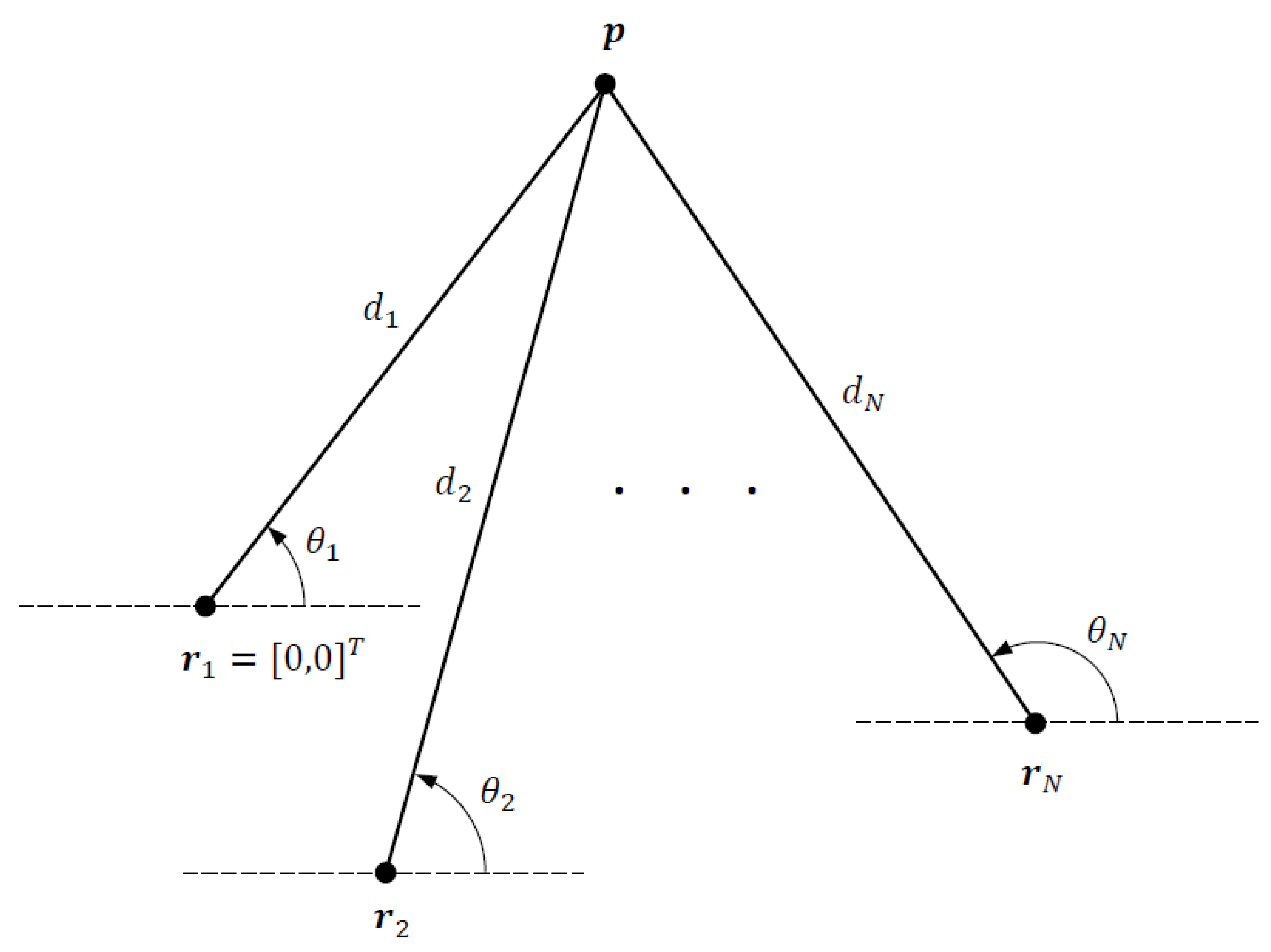
We consider a 2D DRSS-AOA localization problem depicted in Figure 1, where the objective is to estimate the unknown source location $p={[x,y]}^T$ from DRSS and AOA measurements collected by N sensors at fixed and known locations $r_i={[x_i,y_i]}^T$, $i=1,\dots ,N$. The distance between the source and a sensor is given by $d_i=\parallel d_i\parallel$ where $d_i=p-r_i$ and $\parallel ·\parallel$ denotes the Euclidean norm. Letting $r_1$ be the reference sensor location for DRSS measurements, we set $r_1=0$ after appropriate geometric translation with no loss of generality.

Figure 1. DRSS-AOA localization geometry.

The noisy AOA measurements at sensor i are given by

$${\tilde{\theta }}_i={\theta }_i+n_i,i=1,\dots ,N,$$

(1)

where $n_i\sim \mathcal{N}(0,{\sigma }_{{\theta }_i}^2)$ is an independent additive noise with zero mean and variance ${\sigma }_{{\theta }_i}^2$. The true angle ${\theta }_i$ is

$${\theta }_i={tan}^{-1}(y-y_i,x-x_i),{\theta }_i\in (-\pi ,\pi ]$$

(2)

where ${tan}^{-1}$ is the 4-quadrant inverse tangent. The covariance matrix of the AOA measurements $[{\tilde{\theta }}_1,\dots ,{\tilde{\theta }}_N]$ is a diagonal matrix:

$${\mathbf{W}}_{\mathrm{AOA}}=\mathrm{diag}({\sigma }_{{\theta }_1}^2,\dots ,{\sigma }_{{\theta }_N}^2).$$

(3)

The power difference (DRSS) measurements with respect to the reference sensor at $r_1$ follow the propagation path loss model [24,26,29,30,42]

$${\tilde{p}}_{i,1}=p_{i,1}+{ϵ}_{i,1},i=2,\dots ,N,$$

(4)

where $p_{i,1}=10\gamma {log}_{10}\frac{d_1}{d_i}$ is the true power difference between sensor i and the reference sensor (in dBm or dBW), $\gamma$ is the path loss exponent which is assumed known a priori, and ${ϵ}_{i,1}\sim \mathcal{N}(0,{\sigma }_{p_1}^2+{\sigma }_{p_i}^2)$ is the log-normal noise representing shadowing effects with variance ${\sigma }_{p_1}^2+{\sigma }_{p_i}^2$, which is the sum of RSS log-normal noise variances at $r_1$ and $r_i$. The covariance matrix of the DRSS measurements $[{\tilde{p}}_{2,1},\dots ,{\tilde{p}}_{N,1}]$ is

$${\mathbf{W}}_{\mathrm{DRSS}}={\sigma }_{p_1}^2{{\displaystyle 1}}_{N-1}+\mathrm{diag}({\sigma }_{p_2}^2,\dots ,{\sigma }_{p_N}^2)$$

(5)

where $1_{N-1}$ is an $(N-1)\times (N-1)$ matrix of ones.

The $(2N-1)\times 1$ hybrid measurement vector combining the AOA and DRRS measurements is

$$\tilde{\mathbf{\psi }}={\displaystyle \mathbf{\psi }}+{\displaystyle \mathbf{\beta }},$$

(6)

where

$$\tilde{\mathbf{\psi }}={[{\tilde{\theta }}_1,\dots ,{\tilde{\theta }}_N,{\tilde{p}}_{2,1},\dots ,{\tilde{p}}_{N,1}]}^T,$$

(7a)

$${\displaystyle \mathbf{\psi }}={[{\theta }_1,\dots ,,{\theta }_N,p_{2,1},\dots ,p_{N,1}]}^T,$$

(7b)

$${\displaystyle \mathbf{\beta }}={[n_1,\dots ,n_N,{ϵ}_{2,1},\dots ,{ϵ}_{N,1}]}^T.$$

(7c)

The covariance matrix of $\mathbf{\beta }$ is a $(2N-1)\times (2N-1)$ block-diagonal matrix

$$\mathbf{W}=\mathbb{E}\left\{{\displaystyle \mathbf{\beta }}{{\displaystyle \mathbf{\beta }}}^T\right\}=\left[\begin{array}{cc}{\mathbf{W}}_{AOA}& {\displaystyle 0}\\ {\displaystyle 0}& {\mathbf{W}}_{DRSS}\end{array}\right].$$

(8)

Observe that the AOA and DRSS measurement errors are not correlated. This is because the AOA measurement errors arise from thermal noise and possibly some interference at sensors while the log-normal noise in DRSS measurements is caused by shadowing. The two noise sources are physically independent phenomena.

3. Maximum Likelihood Estimator

The likelihood function for the hybrid measurements is a multivariate Gaussian pdf [43], which is given by

$$\begin{array}{cc}\hfill p\left(\tilde{\mathbf{\psi }}\right|\widehat{p})& =\frac{1}{{\left(2\pi \right)}^{(2N-1)/2}{\left|\mathbf{W}\right|}^{1/2}}\hfill \\ & \times exp\left\{-\frac{1}{2}{(\tilde{\mathbf{\psi }}-{\displaystyle \mathbf{\psi }}\left(\widehat{p}\right))}^T{\mathbf{W}}^{-1}(\tilde{\mathbf{\psi }}-{\displaystyle \mathbf{\psi }}\left(\widehat{p}\right))\right\},\hfill \end{array}$$

(9)

where $|·|$ denotes matrix determinant or scalar absolute value, and

$${\displaystyle \mathbf{\psi }}\left(\widehat{p}\right)={[{\theta }_1\left(\widehat{p}\right),\dots ,,{\theta }_N\left(\widehat{p}\right),p_{2,1}\left(\widehat{p}\right),\dots ,p_{N,1}\left(\widehat{p}\right)]}^T$$

(10)

is the $(2N-1)\times 1$ vector of DRSS-AOA estimates constructed by substituting the estimated source location $\widehat{p}={[\widehat{x},\widehat{y}]}^T$ for the true source location $p$:

$${\theta }_i\left(\widehat{p}\right)={tan}^{-1}(\widehat{y}-y_i,\widehat{x}-x_i),{\theta }_i\left(\widehat{p}\right)\in (-\pi ,\pi ],i=1,\dots ,N,$$

(11a)

$$p_{i,1}\left(\widehat{p}\right)=-10\gamma {log}_{10}\frac{\parallel \widehat{p}-r_i\parallel }{\parallel \widehat{p}\parallel },i=2,\dots ,N.$$

(11b)

The maximum likelihood estimate (MLE) of the source location is obtained by maximizing the log-likelihood function $lnp\left(\tilde{\mathbf{\psi }}\right|\widehat{p})$ over $\widehat{p}$, which is equivalent to

$${\widehat{p}}_{ML}=\underset{p\in {\mathbb{R}}^2}{arg\; min}{{\displaystyle h}}^T\left({\displaystyle p}\right){\mathbf{W}}^{-1}{\displaystyle h}\left({\displaystyle p}\right),$$

(12)

where

$${\displaystyle h}\left({\displaystyle p}\right)=\tilde{\mathbf{\psi }}-{\displaystyle \mathbf{\psi }}\left({\displaystyle p}\right).$$

(13)

The nonlinear minimization problem in (12) can be solved numerically by an iterative search algorithm such as the steepest-descent, Levenberg–Marquardt, trust region and Gauss–Newton method [44]. In this paper, the Gauss–Newton method is adopted, which calculates the MLE using the following iterations:

$$\widehat{p}(j+1)=\widehat{p}\left(j\right)+{\left({\mathbf{J}}^T\left(j\right){\mathbf{W}}^{-1}\mathbf{J}\left(j\right)\right)}^{-1}{\mathbf{J}}^T\left(j\right){\mathbf{W}}^{-1}{\displaystyle h}\left(\widehat{p}\left(j\right)\right),j=0,1,\dots$$

(14)

Here $\mathbf{J}\left(j\right)$ is the $(2N-1)\times 2$ Jacobian matrix of $\mathbf{\psi }\left(\widehat{p}\right)$ evaluated at $p=\widehat{p}\left(j\right)$:

$$\mathbf{J}\left(j\right)={[{{\displaystyle J}}_{{\theta }_1}^T\left(j\right),\dots ,{{\displaystyle J}}_{{\theta }_N}^T\left(j\right),{{\displaystyle J}}_{p_{2,1}}^T\left(j\right),\dots ,{{\displaystyle J}}_{p_{N,1}}^T\left(j\right)]}^T,$$

(15)

where

$${{\displaystyle J}}_{{\theta }_k}\left(j\right)=\frac{[-sin{\theta }_i\left(\widehat{p}\left(j\right)\right),cos{\theta }_i\left(\widehat{p}\left(j\right)\right)]}{\parallel \widehat{p}\left(j\right)-r_i\parallel },i=1,\dots ,N$$

(16a)

$$\begin{array}{cc}\hfill {{\displaystyle J}}_{p_{i,1}}\left(j\right)& =\frac{10\gamma }{ln\left(10\right)}\left(\frac{{(r_i-\widehat{p}\left(j\right))}^T}{\parallel r_i-\widehat{p}{\left(j\right)\parallel }_2^2}+\frac{{\widehat{p}}^T\left(j\right)}{\parallel \widehat{p}{\left(j\right)\parallel }_2^2}\right)\hfill \\ \hfill & =\frac{10\gamma }{ln\left(10\right)}{\left[\begin{array}{c}-\frac{cos{\theta }_i\left(\widehat{p}\left(j\right)\right)}{\parallel \widehat{p}\left(j\right)-r_i\parallel }+\frac{cos{\theta }_1\left(\widehat{p}\left(j\right)\right)}{\parallel \widehat{p}\left(j\right)\parallel }\\ -\frac{sin{\theta }_i\left(\widehat{p}\left(j\right)\right)}{\parallel \widehat{p}\left(j\right)-r_i\parallel }+\frac{sin{\theta }_1\widehat{p}\left(j\right)}{\parallel \widehat{p}\left(j\right)\parallel }\end{array}\right]}^T,i=2,3\dots ,N.\hfill \end{array}$$

(16b)

The GN is initialized by $\widehat{p}\left(0\right)$, which needs to be selected carefully.

Being asymptotically efficient and unbiased, the MLE is often considered to be a benchmark in performance comparisons. However, the iterative methods used in MLE calculation can diverge if they are poorly initialized or the noise is too large, causing threshold effects (sharp degradation in estimation performance as the measurement noise increases above a threshold value). Furthermore, the MLE algorithms have a large computational complexity.

The Cramer–Rao lower bound for the hybrid DRSS-AOA localization problem is given by [43]

$$\mathrm{CRLB}={\left({\mathbf{J}}_0^T{\mathbf{W}}^{-1}{\mathbf{J}}_0\right)}^{-1},$$

(17)

where ${\mathbf{J}}_0$ is the Jacobian matrix in (15) evaluated at the true source location $p$.

4. Pseudolinear Equations for Hybrid Measurements

4.1. Linearized AOA Equations

According to [6,40], the pseudolinear form for AOA measurements is

$${\mathbf{A}}_{{\theta }_i}{\displaystyle p}=b_{{\theta }_i}+e_{{\theta }_i},i=1,\dots ,N$$

(18)

where

$${\mathbf{A}}_{{\theta }_i}=[sin{\tilde{\theta }}_i,-cos{\tilde{\theta }}_i],$$

(19a)

$$b_{{\theta }_i}=[sin{\tilde{\theta }}_i,-cos{\tilde{\theta }}_i]{{\displaystyle r}}_i,$$

(19b)

$$e_{{\theta }_i}=d_{i}sin{n}_i\approx d_i{n}_i.$$

(19c)

The approximation in (19c) is valid for sufficiently small AOA measurement noise.

4.2. Linearized DRSS Equations

The DRSS measurement Equation (4) can be rewritten as

$${10}^{\frac{{\tilde{p}}_{i,1}}{10\gamma }}{d}_i={10}^{\frac{{ϵ}_{i,1}}{10\gamma }}{d}_1,i=2,\dots ,N.$$

(20)

Squaring both sides of the above equation yields

$${\mathbf{A}}_{i,1}{\displaystyle y}=b_i+e_i,i=2,\dots ,N$$

(21)

where

$$\begin{array}{cc}\hfill {\mathbf{A}}_{i,1}& =[-2\times {10}^{\frac{{\tilde{p}}_{i,1}}{5\gamma }}{{\displaystyle r}}_i^T,{10}^{\frac{{\tilde{p}}_{i,1}}{5\gamma }}-1]\hfill \end{array}$$

(22a)

$$\begin{array}{cc}\hfill {\displaystyle y}& =\left[\begin{array}{c}{\displaystyle p}\\ {\parallel {\displaystyle p}\parallel }^2\end{array}\right]\hfill \end{array}$$

(22b)

$$\begin{array}{cc}\hfill b_i& =-{10}^{\frac{{\tilde{p}}_{i,1}}{5\gamma }}{\parallel {{\displaystyle r}}_i\parallel }^2\hfill \end{array}$$

(22c)

$$\begin{array}{cc}\hfill e_i& =\left({10}^{\frac{{ϵ}_{i,1}}{5\gamma }}-1\right)d_1^2\hfill \end{array}$$

(22d)

A key challenge with the linearized DRSS Equation (21) is the presence of a nuisance parameter, viz., ${\parallel p\parallel }^2$, in $y$, that depends on the source location, thereby creating an undesirable nonlinear constraint in the solution. This constraint must be imposed on the estimate of $y$ to assure good estimation performance.

4.3. Linearized DRSS-AOA Equations

Here we show how the nuisance parameter in the linearized DRSS equation can be eliminated by using hybrid DRSS-AOA measurements, leading to a linear matrix equation free of nuisance parameter and nonlinear constraints. To do this, first consider the noiseless DRSS equation

$$p_{i,1}=-10\gamma {log}_{10}\frac{d_i}{d_1},i=2,\dots ,N$$

(23)

which can be rewritten as

$${10}^{-\frac{p_{i,1}}{10\gamma }}\parallel {\displaystyle p}\parallel =d_i.$$

(24)

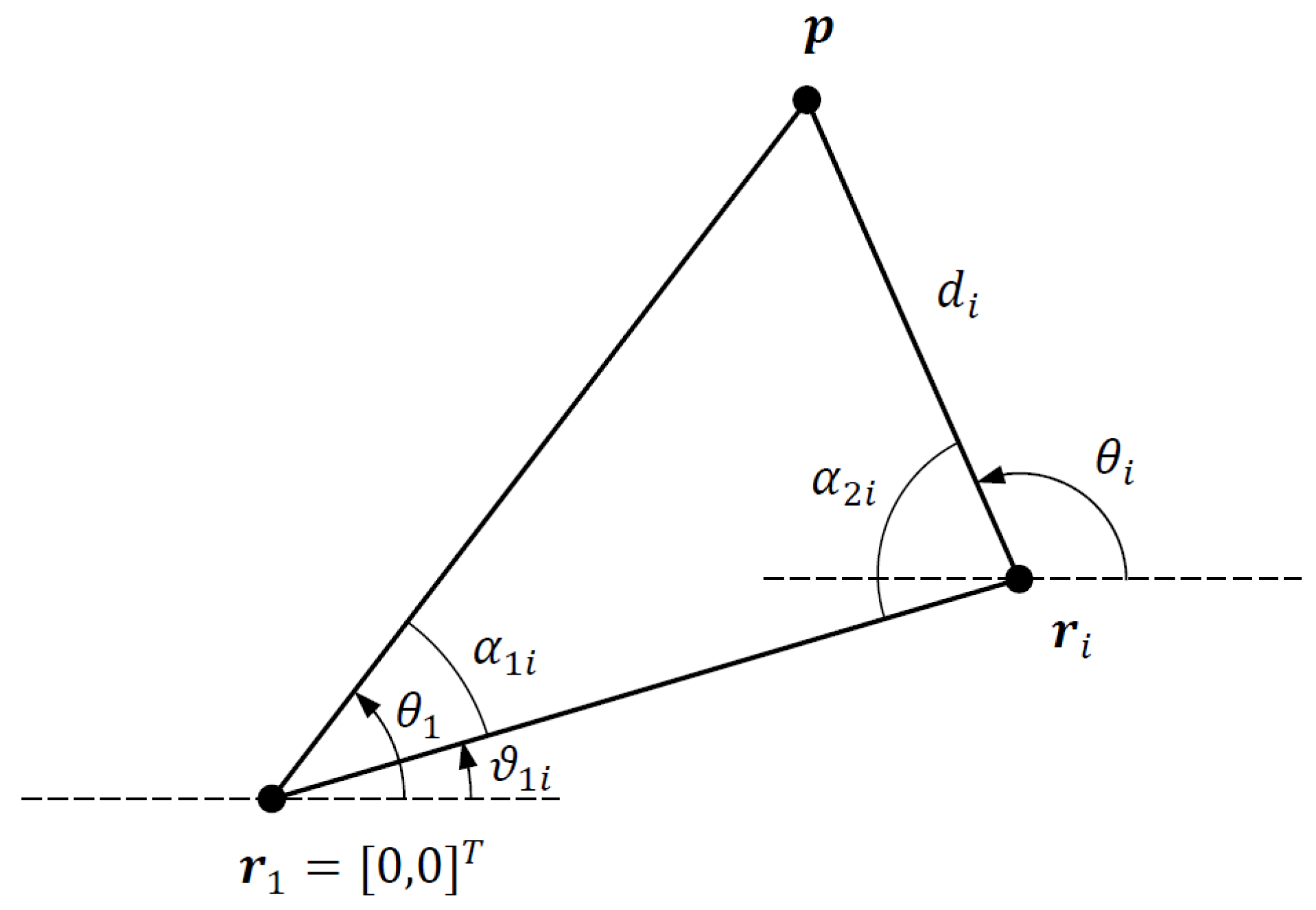
Next, consider the triangle formed by the corner points $p$, $r_1$ and $r_i$, which shown in Figure 2. From the dot products $r_i·p$ and $r_i·d_i$, we obtain

$$cos{\alpha }_{1i}=\frac{r_i^{T}p}{\parallel r_i\parallel \parallel p\parallel }\Rightarrow \parallel {\displaystyle p}\parallel =\frac{r_i^{T}p}{\parallel r_i\parallel cos{\alpha }_{1i}},$$

(25a)

$$cos{\alpha }_{2i}=-\frac{r_i^T{d}_i}{\parallel r_i\parallel d_i}\Rightarrow d_i=-\frac{r_i^T{d}_i}{\parallel r_i\parallel cos{\alpha }_{2i}}.$$

(25b)

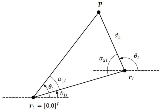
Figure 2. Triangle formed by corner points $p$, $r_1$ and $r_i$.

The angles of the triangle ${\alpha }_{1i}$ and ${\alpha }_{2i}$ are easily obtained from the AOA angles ${\theta }_1$ and ${\theta }_i$ as follows:

$$\begin{array}{cc}\hfill {\vartheta }_{1i}& =\angle {{\displaystyle r}}_i\hfill \end{array}$$

(26a)

$$\begin{array}{cc}\hfill {\alpha }_{1i}& ={\theta }_1-{\vartheta }_{1i},-\pi <{\alpha }_{1i}\le \pi \hfill \end{array}$$

(26b)

$$\begin{array}{cc}\hfill {\alpha }_{2i}& =\pi -{\theta }_i+{\vartheta }_{1i},-\pi <{\alpha }_{2i}\le \pi \hfill \end{array}$$

(26c)

where ∠ denotes the vector angle. Note that both ${\alpha }_{1i}$ and ${\alpha }_{2i}$ are wrapped to the interval $(-\pi ,\pi ]$.

Substituting (25a) and (25b) into (24) yields

$$\begin{array}{c}{10}^{-\frac{p_{i,1}}{10\gamma }}\frac{r_i^{T}p}{\parallel r_i\parallel cos{\alpha }_{1i}}=-\frac{r_i^T{d}_i}{\parallel r_i\parallel cos{\alpha }_{2i}}\end{array}$$

(27a)

$$\begin{array}{c}{10}^{-\frac{p_{i,1}}{10\gamma }}{{\displaystyle r}}_i^T{\displaystyle p}cos{\alpha }_{2i}=-{{\displaystyle r}}_i^T{{\displaystyle d}}_{i}cos{\alpha }_{1i}.\end{array}$$

(27b)

Finally, plugging $d_i=p-r_i$ into (27b), we obtain the following linearized DRSS equation incorporating AOA, which is free of nuisance parameter:

$${\overline{\mathbf{A}}}_{p_{i,1}}{\displaystyle p}={\overline{b}}_{p_{i,1}}$$

(28)

where

$${\overline{\mathbf{A}}}_{p_{i,1}}=\left({10}^{-\frac{p_{i,1}}{10\gamma }}cos{\alpha }_{2i}+cos{\alpha }_{1i}\right){{\displaystyle r}}_i^T$$

and

$${\overline{b}}_{p_{i,1}}={\parallel {{\displaystyle r}}_i\parallel }^{2}cos{\alpha }_{1i}.$$

Replacing the true AOA and DRSS values with noisy measurements, (28) becomes

$${\mathbf{A}}_{p_{i,1}}{\displaystyle p}=b_{p_{i,1}}+e_{p_{i,1}},$$

(29)

where $e_{p_{i,1}}$ is given by (A5) in Appendix A, and

$$\begin{array}{cc}\hfill {\mathbf{A}}_{p_{i,1}}& =\left({10}^{-\frac{{\tilde{p}}_{i,1}}{10\gamma }}cos{\tilde{\alpha }}_{2i}+cos{\tilde{\alpha }}_{1i}\right){{\displaystyle r}}_i^T\hfill \end{array}$$

(30a)

$$\begin{array}{cc}\hfill b_{p_{i,1}}& =\parallel {{\displaystyle r}}_i{\parallel }^{2}cos{\tilde{\alpha }}_{1i}\hfill \end{array}$$

(30b)

$$\begin{array}{cc}\hfill {\tilde{\alpha }}_{1i}& ={\alpha }_{1i}+n_1\hfill \end{array}$$

(30c)

$$\begin{array}{cc}\hfill {\tilde{\alpha }}_{2i}& ={\alpha }_{2i}-n_i.\hfill \end{array}$$

(30d)

As AOA and DRSS measurement errors are zero mean, we have

$$\mathbb{E}\left\{e_{p_{i,k}}\right\}\approx 0.$$

(31)

Stacking N AOA measurements and $N-1$ DRSS measurements, we obtain the linearized DRSS-AOA matrix equation:

$$\mathbf{A}{\displaystyle p}={\displaystyle b}+{\displaystyle e},$$

(32)

where

$$\begin{array}{cc}\hfill \mathbf{A}& ={[{\mathbf{A}}_{{\theta }_1}^T,\cdots ,{\mathbf{A}}_{{\theta }_N}^T,{\mathbf{A}}_{p_{2,1}}^T,\cdots ,{\mathbf{A}}_{p_{N,1}}^T]}^T,\hfill \end{array}$$

(33a)

$$\begin{array}{cc}\hfill {\displaystyle b}& ={[b_{{\theta }_1},\cdots ,b_{{\theta }_N},b_{p_{2,1}},\cdots ,b_{p_{N,1}}]}^T,\hfill \end{array}$$

(33b)

$$\begin{array}{cc}\hfill {\displaystyle e}& ={[e_{{\theta }_1},\cdots ,e_{{\theta }_N},e_{p_{2,1}},\cdots ,e_{p_{N,1}}]}^T\hfill \end{array}$$

(33c)

and

$$\mathbb{E}\left\{{\displaystyle e}\right\}\approx {\displaystyle 0}.$$

(34)

Note that (32) does not have a nuisance parameter. Therefore it can be solved without any constraint on the unknown vector as described in the next section.

5. Hybrid Pseudolinear Estimators

5.1. LS Solution and Bias Analysis

The least-squares solution for the linear matrix equation $\mathbf{A}p\approx b$ (see (32)) is [43]

$$\begin{array}{cc}\hfill {\widehat{p}}_{LS}& =\underset{p\in {\mathbb{R}}^2}{arg\; min}{\parallel \mathbf{A}{\displaystyle p}-{\displaystyle b}\parallel }^2\hfill \end{array}$$

(35a)

$$\begin{array}{cc}\hfill & ={\left({\mathbf{A}}^T\mathbf{A}\right)}^{-1}{\mathbf{A}}^T{\displaystyle b}.\hfill \end{array}$$

(35b)

Substituting (32) into (35b), the least-squares estimate in terms of the pseudolinear noise vector $e$ can be written as

$$\begin{array}{cc}\hfill {\widehat{p}}_{LS}& ={\left({\mathbf{A}}^T\mathbf{A}\right)}^{-1}{\mathbf{A}}^T{\displaystyle b}\hfill \\ \hfill & ={\left({\mathbf{A}}^T\mathbf{A}\right)}^{-1}{\mathbf{A}}^T(\mathbf{A}{\displaystyle p}-{\displaystyle e})\hfill \\ \hfill & ={\displaystyle p}-{\left({\mathbf{A}}^T\mathbf{A}\right)}^{-1}{\mathbf{A}}^T{\displaystyle e}.\hfill \end{array}$$

(36)

The least-squares estimation bias is

$${{\displaystyle \mathbf{\delta }}}_{\mathrm{LS}}=\mathbb{E}\left\{{\widehat{p}}_{\mathrm{LS}}\right\}-{\displaystyle p}=-\mathbb{E}\left\{{\left({\mathbf{A}}^{\mathbf{T}}\mathbf{A}\right)}^{-1}{\mathbf{A}}^T{\displaystyle e}\right\},$$

(37)

and the error covariance matrix of the estimate is

$$\begin{array}{cc}\hfill {\mathbf{C}}_{\mathrm{LS}}& =\mathbb{E}\left\{({\widehat{p}}_{LS}-{\displaystyle p}){({\widehat{p}}_{LS}-{\displaystyle p})}^T\right\}\hfill \\ \hfill & =\mathbb{E}\left\{{\left({\mathbf{A}}^T\mathbf{A}\right)}^{-1}{\mathbf{A}}^T{\displaystyle e{e}^T}\mathbf{A}{\left({\mathbf{A}}^T\mathbf{A}\right)}^{-1}\right\}.\hfill \end{array}$$

(38)

For sufficiently large N and under mild assumptions, Slutsky’s theorem [45] allows (37) to be approximated by the product of expectations:

$${{\displaystyle \mathbf{\delta }}}_{\mathrm{LS}}\approx -\mathbb{E}{\left\{\frac{{\mathbf{A}}^T\mathbf{A}}{2N-1}\right\}}^{-1}\mathbb{E}\left\{\frac{{\mathbf{A}}^{T}e}{2N-1}\right\}.$$

(39)

Using (33), the cross-correlation between $\mathbf{A}$ and $e$ is

$$\mathbb{E}\left\{{\mathbf{A}}^T{\displaystyle e}\right\}=\sum _{i=1}^N\mathbb{E}\left\{{\mathbf{A}}_{{\theta }_i}^T{e}_{{\theta }_i}\right\}+\sum _{i=2}^N\mathbb{E}\left\{{\mathbf{A}}_{p_{i,1}}^T{e}_{p_{i,1}}\right\}.$$

(40)

According to (19a) and (19c), even for small AOA noise, we have [40]

$$\mathbb{E}\left\{{\mathbf{A}}_{{\theta }_i}^T{e}_{{\theta }_i}\right\}\approx {\sigma }_{{\theta }_i}^2{{\displaystyle d}}_i\ne {\displaystyle 0}.$$

(41)

An approximate expression for $\mathbb{E}\left\{{\mathbf{A}}_{p_{i,1}}^T{e}_{p_{i,1}}\right\}$ can be derived from (30a) and (A4). Firstly, expanding the cosine terms of ${\mathbf{A}}_{p_{i,1}}$ and approximating ${\mathbf{A}}_{p_{i,1}}$ using (A3), we obtain

$$\begin{array}{cc}\hfill {\mathbf{A}}_{p_{i,1}}& \approx (C_{1i}cos{\alpha }_{2i}+cos{\alpha }_{1i}-C_{2i}{ϵ}_{i,1}cos{\alpha }_{2i}\hfill \\ \hfill & +C_{1i}{n}_{i}sin{\alpha }_{2i}-n_{1}sin{\alpha }_{1i}\hfill \\ \hfill & -C_{1i}\frac{n_i^2}{2}cos{\alpha }_{2i}+C_{3i}{ϵ}_{i,1}^{2}cos{\alpha }_{2i}\hfill \\ \hfill & -C_{2i}{n}_i{ϵ}_{i,1}sin{\alpha }_{2i}-\frac{n_1^2}{2}cos{\alpha }_{1i}\hfill \\ \hfill & +C_{2i}\frac{n_i^2}{2}{ϵ}_{i,1}cos{\alpha }_{2i}+C_{3i}{n}_i{ϵ}_{i,1}^{2}sin{\alpha }_{2i}\hfill \\ \hfill & -C_{3i}\frac{n_i^2}{2}{ϵ}_{i,1}^{2}cos{\alpha }_{2i}){{\displaystyle r}}_i^T.\hfill \end{array}$$

(42)

Taking the expectation of ${\mathbf{A}}_{p_{i,1}}^T{e}_{p_{i,1}}$ yields

$$\begin{array}{cc}\hfill \mathbb{E}\left\{{\mathbf{A}}_{p_{i,1}}^T{e}_{p_{i,1}}\right\}& \approx (-C_{1i}^2\parallel {{\displaystyle r}}_i\parallel \frac{{\sigma }_{{\theta }_i}^2}{2}{cos}^2{\alpha }_{2i}-C_{1i}\parallel {{\displaystyle r}}_i\parallel \frac{{\sigma }_{{\theta }_i}^2}{2}cos{\alpha }_{2i}cos{\alpha }_{1i}\hfill \\ \hfill & +3C_{1i}{C}_{3i}\parallel {{\displaystyle r}}_i\parallel {\sigma }_{p_{i,1}}^2{cos}^2{\alpha }_{2i}+C_{3i}\parallel {{\displaystyle r}}_i\parallel {\sigma }_{p_{i,1}}^{2}cos{\alpha }_{2i}cos{\alpha }_{1i}\hfill \\ \hfill & +C_{1i}^2\parallel {{\displaystyle d}}_i\parallel \frac{{\sigma }_{{\theta }_i}^2}{2}{cos}^3{\alpha }_{2i}+C_{1i}\parallel {{\displaystyle d}}_i\parallel \frac{{\sigma }_{{\theta }_i}^2}{2}{cos}^2{\alpha }_{2i}cos{\alpha }_{1i}\hfill \\ & -3C_{1i}{C}_{3i}\parallel {{\displaystyle d}}_i\parallel {\sigma }_{p_{i,1}}^2{cos}^3{\alpha }_{2i}-C_{3i}\parallel {{\displaystyle d}}_i\parallel {\sigma }_{p_{i,1}}^2{cos}^2{\alpha }_{2i}cos{\alpha }_{1i}\hfill \\ \hfill & -C_{1i}^2\parallel {{\displaystyle d}}_i\parallel {\sigma }_{{\theta }_i}^2{sin}^2{\alpha }_{2i}cos{\alpha }_{2i}+C_{1i}\parallel {{\displaystyle r}}_i\parallel \frac{{\sigma }_{{\theta }_1}^2}{2}cos{\alpha }_{2i}cos{\alpha }_{1i}\hfill \\ \hfill & +\parallel {{\displaystyle r}}_i\parallel \frac{{\sigma }_{{\theta }_1}^2}{2}{cos}^2{\alpha }_{1i}-C_{1i}\parallel {\displaystyle p}\parallel \frac{{\sigma }_{{\theta }_1}^2}{2}cos{\alpha }_{2i}{cos}^2{\alpha }_{1i}\hfill \\ \hfill & -\parallel {\displaystyle p}\parallel \frac{{\sigma }_{{\theta }_1}^2}{2}{cos}^3{\alpha }_{1i}+\parallel {\displaystyle p}\parallel {\sigma }_{{\theta }_1}^2{sin}^2{\alpha }_{1i}cos{\alpha }_{1i}\hfill \\ \hfill & +C_{1i}^2\parallel {{\displaystyle r}}_i\parallel {\sigma }_{{\theta }_i}^2{sin}^2{\alpha }_{2i}-\parallel {{\displaystyle r}}_i\parallel {\sigma }_{{\theta }_1}^2{sin}^2{\alpha }_{1i})\parallel {{\displaystyle r}}_i\parallel {{\displaystyle r}}_i^T\hfill \end{array}$$

(43)

It is clear that $\mathbb{E}\left\{{\mathbf{A}}_{p_{i,1}}^T{e}_{p_{i,1}}\right\}$ cannot be guaranteed to be zero for all $i=2,\dots ,N$. Thus, $\mathbb{E}\left\{{\mathbf{A}}_{p_{i,1}}^T{e}_{p_{i,1}}\right\}\ne 0$.

Based on (41) and (43), we conclude that

$$\mathbb{E}\left\{{\mathbf{A}}^T{\displaystyle e}\right\}=\sum _{i=1}^N\mathbb{E}\left\{{\mathbf{A}}_{{\theta }_i}^T{e}_{{\theta }_i}\right\}+\sum _{i=2}^N\mathbb{E}\left\{{\mathbf{A}}_{p_{i,1}}^T{e}_{p_{i,1}}\right\}\ne {\displaystyle 0}$$

(44)

which means ${\mathbf{\delta }}_{LS}\ne 0$ and the least-squares estimate (35b) is biased.

5.2. WLS Solution and Bias Analysis

The weighted least-squares estimate for $p$ is obtained from [43]

$$\begin{array}{cc}\hfill {\widehat{p}}_{\mathrm{WLS}}& =\underset{p\in {\mathbb{R}}^2}{arg\; min}{\left(\mathbf{A}{\displaystyle p}-{\displaystyle b}\right)}^T{\mathbf{W}}_{\mathrm{PLE}}^{-1}\left(\mathbf{A}{\displaystyle p}-{\displaystyle b}\right)\hfill \end{array}$$

(45a)

$$\begin{array}{cc}\hfill & ={\left({\mathbf{A}}^T{\mathbf{W}}_{PLE}^{-1}\mathbf{A}\right)}^{-1}{\mathbf{A}}^T{\mathbf{W}}_{PLE}^{-1}{\displaystyle b}.\hfill \end{array}$$

(45b)

where ${\mathbf{W}}_{\mathrm{PLE}}$ is the weighting matrix that approximates the covariance of the noise vector $e$:

$${\mathbf{W}}_{\mathrm{PLE}}=\mathbb{E}\left\{{\displaystyle e}{{\displaystyle e}}^T\right\}=\left[\begin{array}{ccc}{W}_{11}& {\mathbf{W}}_{12}& {\mathbf{W}}_{13}\\ {\mathbf{W}}_{12}^T& {\mathbf{W}}_{22}& {\mathbf{W}}_{23}\\ {\mathbf{W}}_{13}^T& {\mathbf{W}}_{23}^T& {\mathbf{W}}_{33}\end{array}\right].$$

(46)

The entries of ${\mathbf{W}}_{\mathrm{PLE}}$ are given by

$$\begin{array}{cc}\hfill W_{11}& =\mathbb{E}\left\{e_{{\theta }_{1,k}}^2\right\}\approx {\parallel {\displaystyle p}\parallel }^2{\sigma }_{{\theta }_1}^2,\hfill \end{array}$$

(47a)

$$\begin{array}{cc}\hfill {\mathbf{W}}_{12}& =\mathbb{E}\left\{e_{{\theta }_{1,k}}[e_{{\theta }_{2,k}},\dots ,e_{{\theta }_{N,k}}]\right\}={{\displaystyle 0}}_{1\times (N-1)},\hfill \\ \hfill {\mathbf{W}}_{13}& =\mathbb{E}\left\{e_{{\theta }_1}[e_{p_{2,1}},\dots ,e_{p_{N,1}}]\right\}\hfill \\ \hfill & \approx [\parallel {{\displaystyle r}}_2{\parallel }^2\parallel {\displaystyle p}\parallel sin{\alpha }_{12}-\parallel {{\displaystyle r}}_2{\parallel \parallel {\displaystyle p}\parallel }^{2}sin{\alpha }_{12}cos{\alpha }_{12},\hfill \\ \hfill & \dots ,\parallel {{\displaystyle r}}_N{\parallel }^2\parallel {\displaystyle p}\parallel sin{\alpha }_{1N}-\parallel {{\displaystyle r}}_N{\parallel \parallel {\displaystyle p}\parallel }^{2}sin{\alpha }_{1N}cos{\alpha }_{1N}]{\sigma }_{{\theta }_1}^2\hfill \end{array}$$

(47b)

$$\begin{array}{cc}\hfill {\mathbf{W}}_{22}& =\mathbb{E}\left\{{[e_{{\theta }_2},\dots ,e_{{\theta }_N}]}^T[e_{{\theta }_2},\dots ,e_{{\theta }_N}]\right\}\hfill \\ \hfill & \approx diag(\dots ,\parallel {{\displaystyle d}}_i{{\parallel }^2{\sigma }_{{\theta }_i}^2,\dots )}_{i=2,\dots ,N},\hfill \end{array}$$

(47c)

$$\begin{array}{cc}\hfill {\mathbf{W}}_{23}& =\mathbb{E}\left\{{[e_{{\theta }_2},\dots ,e_{{\theta }_N}]}^T[e_{p_{2,1}},\dots ,e_{p_{N,1}}]\right\}\hfill \\ \hfill & \approx diag(\dots ,(C_{1i}\parallel {{\displaystyle r}}_i{\parallel }^2\parallel {{\displaystyle d}}_i\parallel sin{\alpha }_{2i}\hfill \\ \hfill & -C_{1i}\parallel {{\displaystyle r}}_i\parallel \parallel {{\displaystyle d}}_i{\parallel }^{2}sin{\alpha }_{2i}cos{\alpha }_{2i}){\sigma }_{{\theta }_i}^2,\dots {)}_{i=2,\dots ,N}\hfill \end{array}$$

(47d)

$$\begin{array}{cc}\hfill {\mathbf{W}}_{33}& =\mathbb{E}\left\{{[e_{p_{2,1}},\dots ,e_{p_{N,1}}]}^T[e_{p_{2,1}},\dots ,e_{p_{N,1}}]\right\}\hfill \\ \hfill & ={[{\beta }_{2,1},\dots ,{\beta }_{N,1}]}^T[{\beta }_{2,1},\dots ,{\beta }_{N,1}]{\sigma }_{{\theta }_1}^2\hfill \\ \hfill & +diag(\dots ,(C_{1i}{\parallel {{\displaystyle r}}_i\parallel }^{2}sin{\alpha }_{2i}\hfill \\ & -C_{1i}\parallel {{\displaystyle r}}_i\parallel \parallel {{\displaystyle d}}_i\parallel sin{\alpha }_{2i}cos{\alpha }_{2i}{)}^2{\sigma }_{{\theta }_i}^2,\dots {)}_{i=2,\dots ,N}\hfill \end{array}$$

(47e)

$$\begin{array}{cc}\hfill & +{[{\eta }_{2,1},\dots ,{\eta }_{N,1}]}^T[{\eta }_{2,1},\dots ,{\eta }_{N,1}]{\mathbf{W}}_{\mathrm{DRSS}}.\hfill \end{array}$$

(47f)

where

$${\beta }_{2,i}=\parallel {{\displaystyle r}}_i{\parallel }^{2}sin{\alpha }_{1i}-\parallel {{\displaystyle r}}_i\parallel \parallel {\displaystyle p}\parallel sin{\alpha }_{1i}cos{\alpha }_{1i},$$

(48a)

$${\eta }_{2,i}=C_{2i}\parallel {{\displaystyle r}}_i\parallel \parallel {{\displaystyle d}}_i\parallel {cos}^2{\alpha }_{2i}-C_{2i}{\parallel {{\displaystyle r}}_i\parallel }^{2}cos{\alpha }_{2i}.$$

(48b)

Note that $d_i$, $r_i$, ${\alpha }_{1i}$, ${\alpha }_{2i}$, $C_{1i}$ and $C_{2i}$ require prior knowledge of the source location $p$, which is not available. We replace $p$ with ${\widehat{p}}_{\mathrm{LS}}$ to calculate those terms.

Substituting (32) into (45b), we have

$${\widehat{p}}_{WLS}={\displaystyle p}-{\left({\mathbf{A}}^T{\mathbf{W}}_{PLE}^{-1}\mathbf{A}\right)}^{-1}{\mathbf{A}}^T{\mathbf{W}}_{PLE}^{-1}{\displaystyle e}$$

(49)

whence the estimation bias is obtained as

$${\delta }_{\mathrm{WLS}}=\mathbb{E}\left\{{\widehat{p}}_{\mathrm{WLS}}\right\}-{\displaystyle p}=-\mathbb{E}\left\{{\left({\mathbf{A}}^T{\mathbf{W}}_{\mathrm{PLE}}^{-1}\mathbf{A}\right)}^{-1}{\mathbf{A}}^T{\mathbf{W}}_{\mathrm{PLE}}^{-1}{\displaystyle e}\right\}.$$

(50)

Similar to (39), for large N, (50) can be approximated as

$${{\displaystyle \mathbf{\delta }}}_{\mathrm{WLS}}\approx -\mathbb{E}{\left\{\frac{{\mathbf{A}}^T{\mathbf{W}}_{\mathrm{PLE}}^{-1}\mathbf{A}}{2N-1}\right\}}^{-1}\mathbb{E}\left\{\frac{{\mathbf{A}}^T{\mathbf{W}}_{\mathrm{PLE}}^{-1}e}{2N-1}\right\}.$$

(51)

As $\mathbf{A}$ and $e$ are correlated as shown in Section 5.1, $\mathbb{E}\left\{{\mathbf{A}}^T{\mathbf{W}}_{\mathrm{PLE}}^{-1}e\right\}\ne 0$, which implies ${\mathbf{\delta }}_{\mathrm{WLS}}\ne 0$ and the WLS estimate is biased.

5.3. WIV Solution

The bias in the LS and WLS estimates can be significantly reduced by employing the method of instrumental variables. A weighted instrumental variable (WIV) estimator is obtained by introducing an IV matrix $\mathbf{G}$ which is strongly correlated with the matrix $\mathbf{A}$ while being statistically independent of $e$. The WIV solution is given by [45]

$${\widehat{p}}_{WIV}={\left({\mathbf{G}}^T{\mathbf{W}}_{PLE}^{-1}\mathbf{A}\right)}^{-1}{\mathbf{G}}^T{\mathbf{W}}_{PLE}^{-1}{\displaystyle b}.$$

(52)

The IV matrix $\mathbf{G}$ is selected such that $\mathbb{E}\left\{\frac{{\mathbf{G}}^T{\mathbf{W}}_{PLE}^{-1}\mathbf{A}}{2N-1}\right\}$ is nonsingular and $\mathbb{E}\left\{\frac{{\mathbf{G}}^T{\mathbf{W}}_{PLE}^{-1}e}{2N-1}\right\}\to 0$ as $N\to \infty$ [46]. A practical IV matrix that meets these requirements can be constructed from an initial source location estimate, such as the LS or WLS estimate, as described below. This procedure is based on [47]. Consider the following row partitioning of the IV matrix $\mathbf{G}$:

$$\mathbf{G}={[{\mathbf{G}}_{{\theta }_1}^T,\dots ,{\mathbf{G}}_{{\theta }_N}^T,{\mathbf{G}}_{p_{2,1}}^T,\dots ,{\mathbf{G}}_{p_{N,1}}^T]}^T,$$

(53)

where

$$\begin{array}{cc}\hfill {\mathbf{G}}_{{\theta }_i}& =\left[sin{\widehat{\theta }}_i,cos{\widehat{\theta }}_i\right],i=1,\dots ,N\hfill \end{array}$$

(54a)

$$\begin{array}{cc}\hfill {\mathbf{G}}_{p_{j,1}}& =\left({10}^{-\frac{{\widehat{p}}_{j,1}}{10\gamma }}cos{\widehat{\alpha }}_{2j}+cos{\widehat{\alpha }}_{1j}\right){{\displaystyle r}}_j^T,j=2,\dots ,N.\hfill \end{array}$$

(54b)

Here the AOA, triangle angle and DRSS estimates are obtained from the initial source location estimate $\widehat{p}={[\widehat{x},\widehat{y}]}^T$ as

$$\begin{array}{cc}\hfill {\widehat{\theta }}_i& ={tan}^{-1}(\widehat{y}-y_i,\widehat{x}-x_i),{\widehat{\theta }}_i\in (-\pi ,\pi ]\hfill \end{array}$$

(55a)

$$\begin{array}{cc}\hfill {\widehat{\alpha }}_{1j}& ={\widehat{\theta }}_1-{\vartheta }_{1j},-\pi <{\widehat{\alpha }}_{1i}\le \pi \hfill \end{array}$$

(55b)

$$\begin{array}{cc}\hfill {\widehat{\alpha }}_{2j}& =\pi -{\widehat{\theta }}_j+{\vartheta }_{1j},-\pi <{\widehat{\alpha }}_{2j}\le \pi \hfill \end{array}$$

(55c)

$$\begin{array}{cc}\hfill {\widehat{p}}_{j,1}& =10\gamma {log}_{10}\frac{\parallel \widehat{p}\parallel }{\parallel \widehat{p}-r_j\parallel }.\hfill \end{array}$$

(55d)

The bias of the WIV estimate is given by

$$\begin{array}{cc}\hfill {{\displaystyle \mathbf{\delta }}}_{\mathrm{WIV}}& =\mathbb{E}\left\{{\widehat{p}}_{WIV}\right\}-{\displaystyle p}\hfill \\ \hfill & =-\mathbb{E}\left\{{\left({\mathbf{G}}^T{\mathbf{W}}_{\mathrm{PLE}}^{-1}\mathbf{A}\right)}^{-1}{\mathbf{G}}^T{\mathbf{W}}_{\mathrm{PLE}}^{-1}{\displaystyle e}\right\}\hfill \end{array}$$

(56)

which, for sufficiently large N, can be approximated as

$${{\displaystyle \mathbf{\delta }}}_{\mathrm{WIV}}\approx -\mathbb{E}{\left\{\frac{{\mathbf{G}}^T{\mathbf{W}}_{\mathrm{PLE}}^{-1}\mathbf{A}}{2N-1}\right\}}^{-1}\mathbb{E}\left\{\frac{{\mathbf{G}}^T{\mathbf{W}}_{\mathrm{PLE}}^{-1}e}{2N-1}\right\}$$

(57)

where

$$\mathbb{E}\left\{\frac{{\mathbf{G}}^T{\mathbf{W}}_{\mathrm{PLE}}^{-1}e}{2N-1}\right\}\approx {\displaystyle 0}.$$

As a result, ${\mathbf{\delta }}_{\mathrm{WIV}}\approx 0$ and, therefore, the WIV estimate is approximately unbiased.

5.4. SHM-WIV Solution

A selective hybrid measurement method is introduced here to keep the IV matrix $\mathbf{G}$, constructed from an initial source location estimate, and the data matrix $\mathbf{A}$ strongly correlated as there is a high probability that $\mathbf{G}$ and $\mathbf{A}$ lose correlation when the measurement noise is large [18]. The principle of selective hybrid measurements is to decide which rows of $\mathbf{G}$ should remain identical to those of $\mathbf{A}$ based on a measure of difference between them.

Consider the difference between the first N rows of $\mathbf{A}$ and $\mathbf{G}$ corresponding to the AOA measurements:

$$\begin{array}{cc}\hfill {\mathbf{A}}_{{\theta }_i}-{\mathbf{G}}_{{\theta }_i}& =\left[\begin{array}{cc}sin{\tilde{\theta }}_i-sin{\widehat{\theta }}_i,& cos{\tilde{\theta }}_i-cos{\widehat{\theta }}_i\end{array}\right]\hfill \\ \hfill & =2sin\left(\frac{{\tilde{\theta }}_i-{\widehat{\theta }}_i}{2}\right)\left[\begin{array}{cc}cos\left(\frac{{\tilde{\theta }}_i+{\widehat{\theta }}_i}{2}\right),& -sin\left(\frac{{\tilde{\theta }}_i+{\widehat{\theta }}_i}{2}\right)\end{array}\right].\hfill \end{array}$$

(58)

The common factor $sin\left(({\tilde{\theta }}_i-{\widehat{\theta }}_i)/2\right)$ suggests that it will be appropriate to use the angle difference $|{\tilde{\theta }}_i-{\widehat{\theta }}_i|$ as a measure of row difference [18], which leads to the following criterion for using ${\widehat{\theta }}_i$, instead of ${\tilde{\theta }}_i$, in the ith row of the IV matrix $\mathbf{G}$:

$$|{\tilde{\theta }}_i-{\widehat{\theta }}_i|\le {\lambda }_1.$$

(59)

The recommended range of values for the threshold is $5{\sigma }_{{\theta }_i}\le {\lambda }_1\le 20{\sigma }_{{\theta }_i}$, $i=1,\dots ,N$. Following extensive simulation studies, we have concluded that selecting ${\lambda }_1$ in this range achieves the intended effect of making the IV matrix strongly correlated with the data matrix. In general, the larger the angle noise, the larger ${\lambda }_1$ should be.

The row difference between $\mathbf{A}$ and $\mathbf{G}$ for the DRSS measurements is

$$\begin{array}{cc}\hfill {\mathbf{A}}_{p_{i,1}}-{\mathbf{G}}_{p_{i,1}}& =\left({10}^{\frac{{\tilde{p}}_{i,1}}{-10\gamma }}cos{\tilde{\alpha }}_{2i}+cos{\tilde{\alpha }}_{1i}\right){{\displaystyle r}}_i^T-\left({10}^{\frac{{\widehat{p}}_{i,1}}{-10\gamma }}cos{\widehat{\alpha }}_{2i}+cos{\widehat{\alpha }}_{1i}\right){{\displaystyle r}}_i^T\hfill \\ \hfill & =(\left({10}^{\frac{{\tilde{p}}_{i,1}}{-10\gamma }}-{10}^{\frac{{\widehat{p}}_{i,1}}{-10\gamma }}\right)(cos{\tilde{\alpha }}_{2i}-cos{\widehat{\alpha }}_{2i})+\left({10}^{\frac{{\tilde{p}}_{i,1}}{-10\gamma }}-{10}^{\frac{{\widehat{p}}_{i,1}}{-10\gamma }}\right)cos{\widehat{\alpha }}_{2i}\hfill \\ \hfill & +{10}^{\frac{{\widehat{p}}_{i,1}}{-10\gamma }}\left(cos{\tilde{\alpha }}_{2i}-cos{\widehat{\alpha }}_{2i}\right)+(cos{\tilde{\alpha }}_{1i}-cos{\widehat{\alpha }}_{1i})){{\displaystyle r}}_i^T\hfill \end{array}$$

(60)

where the following terms determine the magnitude of difference

$$\begin{array}{c}|{10}^{\frac{{\tilde{p}}_{i,1}}{-10\gamma }}-{10}^{\frac{{\widehat{p}}_{i,1}}{-10\gamma }}|\end{array}$$

(61a)

$$\begin{array}{c}|cos{\tilde{\alpha }}_{1i}-cos{\widehat{\alpha }}_{1i}|=|2sin\left(\frac{{\tilde{\alpha }}_{1i}+{\widehat{\alpha }}_{1i}}{2}\right)sin\left(\frac{{\tilde{\theta }}_i-{\widehat{\theta }}_i}{2}\right)|\end{array}$$

(61b)

$$\begin{array}{c}|cos{\tilde{\alpha }}_{2i}-cos{\widehat{\alpha }}_{2i}|=|2sin\left(\frac{{\tilde{\alpha }}_{2i}+{\widehat{\alpha }}_{2i}}{2}\right)sin\left(\frac{{\tilde{\theta }}_1-{\widehat{\theta }}_1}{2}\right)|.\end{array}$$

(61c)

From (61a) we obtain the following criterion for using ${\widehat{p}}_{i,1}$, instead of ${\tilde{p}}_{i,1}$, in $\mathbf{G}$:

$$\begin{array}{c}\hfill |{\tilde{p}}_{i,1}-{\widehat{p}}_{i,1}|\le {\lambda }_2\end{array}$$

(62)

where the recommended range for ${\lambda }_2$ is $5{\sigma }_{p_{i,1}}\le {\lambda }_2\le 20{\sigma }_{p_{i,1}}$ with ${\sigma }_{p_{i,1}}=\sqrt{{\sigma }_{p_1}^2+{\sigma }_{p_i}^2}$. This range was confirmed to yield satisfactory estimation performance through extensive simulation studies.

Equations (61b) and (61c) result in the same criterion as (59). Thus, applying the difference measures in (59) and (62) to (60) yields the hybrid measurement selection criterion:

$$|{\tilde{p}}_{i,1}-{\widehat{p}}_{i,1}\left|\right|{\tilde{\theta }}_1-{\widehat{\theta }}_1|+|{\tilde{p}}_{i,1}-{\widehat{p}}_{i,1}|+|{\tilde{\theta }}_1-{\widehat{\theta }}_1|+|{\tilde{\theta }}_i-{\widehat{\theta }}_i|\le {\lambda }_1{\lambda }_2+{\lambda }_2+2{\lambda }_1.$$

(63)

We refer to the WIV estimate incorporating (59) and (63) in the construction of the IV matrix $\mathbf{G}$ as the selective hybrid measurement WIV (SHM-WIV) algorithm.

6. Simulation Results

6.1. Simulation Set-Up

The RMSE and bias performance of the MLE, LS, WLS, WIV and SHM-WIV algorithms is compared using Monte Carlo simulations. The simulated network topology has ten sensor nodes at fixed locations and a source, all contained within a 60 m × 60 m region. The path loss exponent is assumed to be $\gamma =4$. The range of AOA and DRSS measurement noise is indicated by a noise index given in Table 1. The average SNR values for AOA and DRSS measurements are also included. AOA and DRSS measurements have different SNR values because the AOA noise power is the variance of the additive thermal (Gaussian) noise and the DRSS measurements are corrupted by the shadowing log-normal noise. The AOA measurements are obtained from an antenna array with $m=10$ elements, using [48]

$${\mathrm{SNR}}_i=\frac{6}{m^3{\sigma }_{{\theta }_i}^2},i=1,\dots ,N$$

(64)

which assumes the Cramer–Rao lower bound is achieved. The DRSS SNR values are for a source with transmit power of 40 dBm (10 W). The MLE uses the iterative Gauss–Newton method with initialization obtained from the LS estimate. The SHM-WIV threshold values are given in Table 2.

Table 1. Noise index for AOA/DRSS measurements.

Index	1	2	3	4	5	6	7
${\sigma }_{{\theta }_i}$ (degrees)	0.1	0.2	0.3	0.4	0.5	0.6	0.7
${\sigma }_{p_{i,1}}$ (dBm)	1	1.5	2	2.5	3	4	5
AOA SNR (dB)	32.95	26.92	23.40	20.90	18.96	17.38	16.04
DRSS SNR (dB)	$-22.70$	$-23.20$	$-23.70$	$-24.20$	$-24.70$	$-25.70$	$-26.70$

Table 2. ${\lambda }_1$ and ${\lambda }_2$ for SHM-WIV.

Noise Index	1	2	3	4	5	6	7
AOA ${\lambda }_1$	$6.5\sigma$	$6.5\sigma$	$6.5\sigma$	$6.5\sigma$	$6.5\sigma$	$18\sigma$	$20\sigma$
DRSS ${\lambda }_2$	$6.5\sigma$	$6.5\sigma$	$6.5\sigma$	$6.5\sigma$	$6.5\sigma$	$18\sigma$	$20\sigma$

6.2. Fixed Source Location

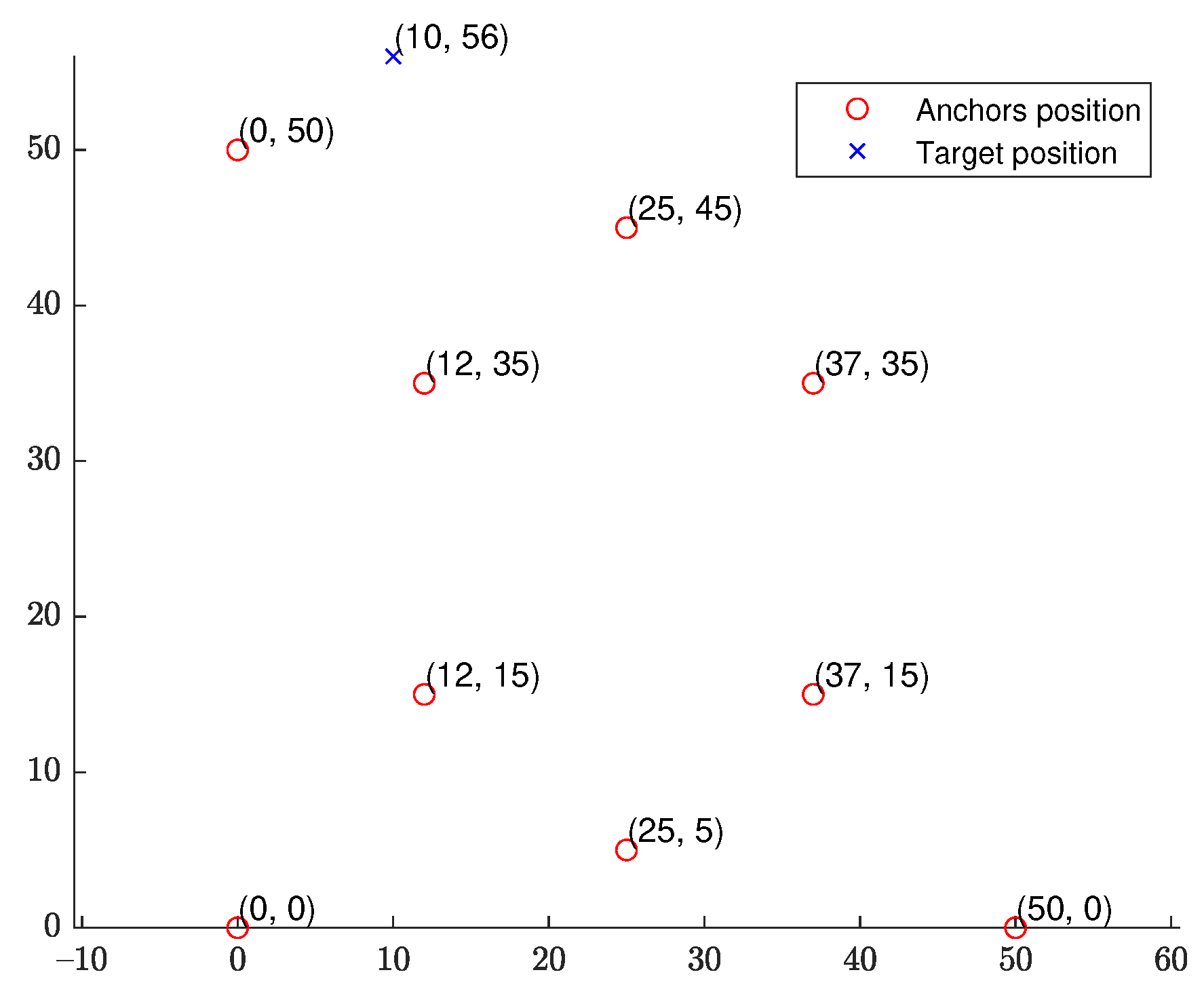
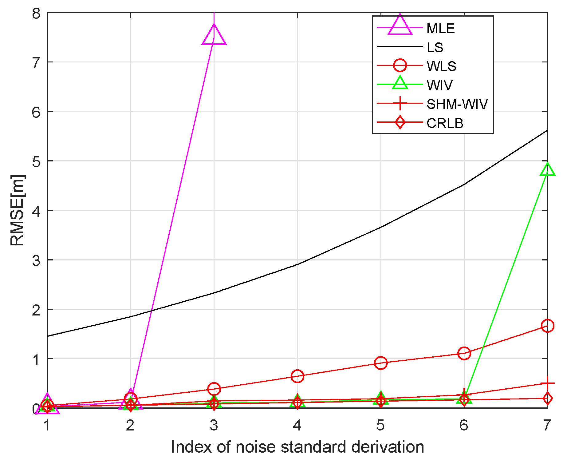
We start with a fixed network topology simulation where the source is stationary at a fixed location $p={[10,56]}^T$ as shown in Figure 3. The simulations consist of 10,000 Monte Carlo runs. Figure 4 and Figure 5 present the RMSE and bias results versus noise index. The MLE achieves the CRLB at small noise (noise index 1 and 2), but starts to diverge for large noise. The LS exhibits significant bias and poor RMSE compared to the other estimates for all noise levels. The WLS has a better bias and RMSE performance than the LS, but still shows a large bias and deviates from the CRLB for large noise. The WIV attains the CRLB when the noise index is below 6, but its RMSE rapidly deviates from the CRLB at noise index 7. The SHM-WIV exhibits the best overall RMSE and bias performance for the entire noise range.

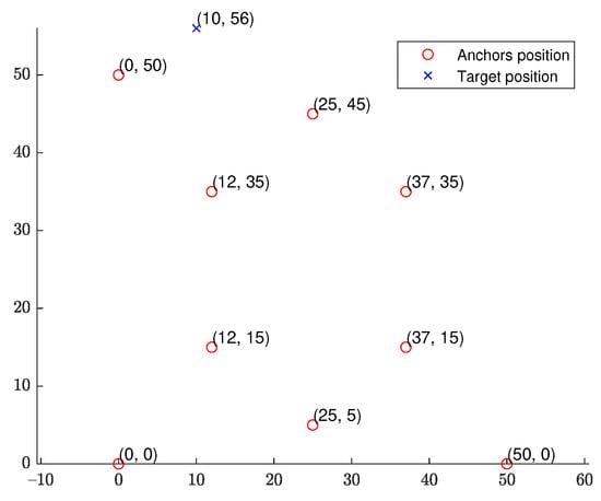
Figure 3. DRSS-AOA geometry with fixed source location.

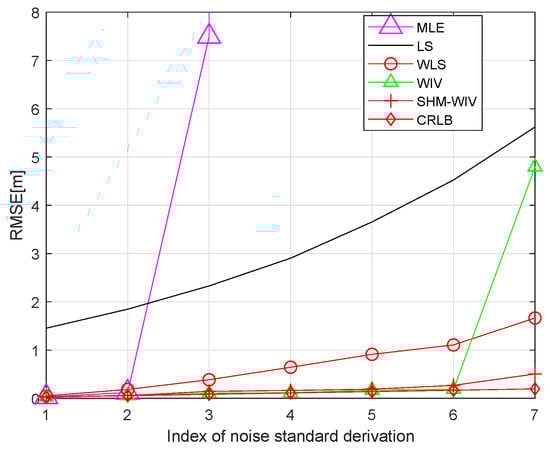
Figure 4. RMSE versus noise with fixed source location.

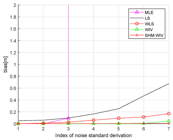
Figure 5. Bias versus noise with fixed source location.

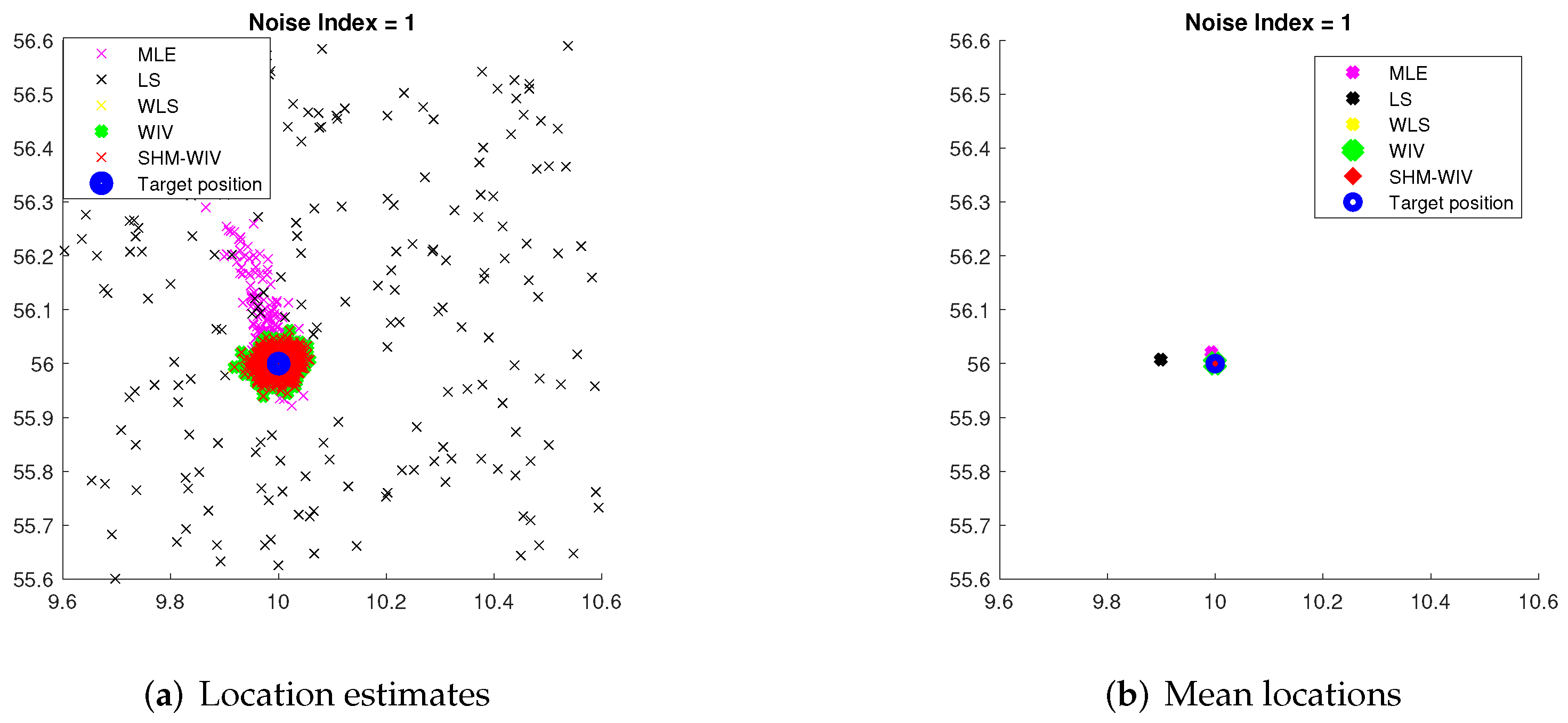
For noise index 1 and 4, individual location estimates along with mean locations for the simulated algorithms are shown in Figure 6 and Figure 7, respectively, to demonstrate the spread of estimates. The standard deviations of Monte Carlo simulation results that led to the bias and RMSE values plotted in Figure 4 and Figure 5 are listed in Table 3. The standard deviation is left blank for algorithms that exhibit divergence.

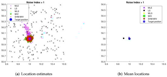
Figure 6. (a) Plot of individual location estimates for noise index 1; (b) Plot of mean location estimates for noise index 1.

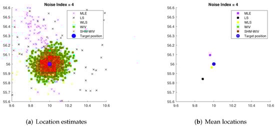
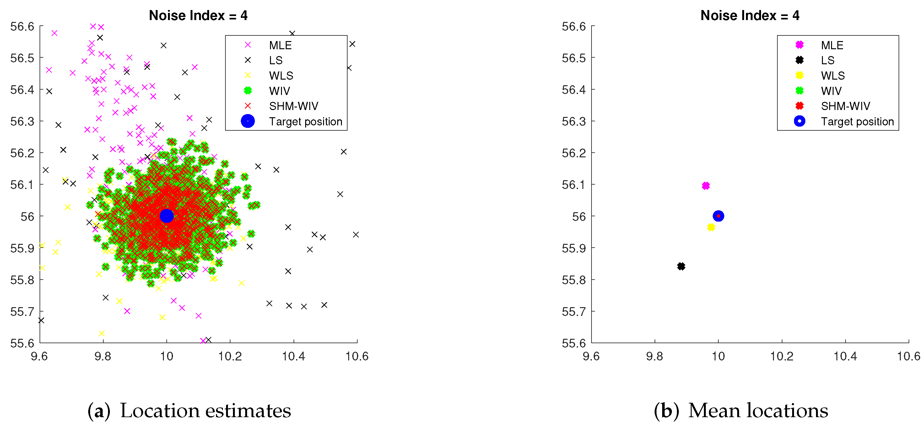
Figure 7. (a) Plot of individual location estimates for noise index 4; (b) Plot of mean location estimates for noise index 4.

Table 3. Standard deviations of Monte Carlo results for bias/RMSE values.

Index	bias/RMSE	MLE	LS	WLS	WIV	SHM-WIV
1	Bias	$0.0007$	$0.0069$	$0.0004$	$0.0002$	$0.0001$
	RMSE	$0.0024$	$0.0098$	$0.0183$	$0.0147$	$0.0044$
2	Bias	$0.0013$	$0.0095$	$0.0013$	$0.0002$	$0.0003$
	RMSE	$0.0037$	$0.0115$	$0.0268$	$0.0019$	$0.0110$
3	Bias	$0.0017$	$0.0113$	$0.0029$	$0.0012$	$0.0008$
	RMSE	$0.0053$	$0.0123$	$0.0351$	$0.1219$	$0.0203$
4	Bias	$0.0033$	$0.0170$	$0.0045$	$0.0018$	$0.0012$
	RMSE	$0.1676$	$0.0159$	$0.0417$	$0.1596$	$0.0237$
5	Bias		$0.0184$	$0.0062$	$0.3103$	$0.0020$
	RMSE		$0.0206$	$0.0503$	$0.4246$	$0.0453$
6	Bias		$0.0233$	$0.0070$	$0.0044$	$0.0041$
	RMSE		$0.0294$	$0.0641$	$0.4337$	$0.4022$
7	Bias		$0.0288$	$0.0125$	$56.8201$	$0.0048$
	RMSE		$0.0302$	$0.0771$	5682	$0.4105$

The total run times of the simulated algorithms are listed in Table 4. We observe that the LS runs the fastest; however, it has a poor performance. The WLS is approximately three times slower than the LS due to weighting matrix computation. The MLE and WLS have comparable run times, even though the Gauss–Newton iterations can take longer time depending on initialization. The WIV is roughly five times slower than the LS because of computational overheads associated with weighting matrix and IV matrix computations. The SHM-WIV is slightly slower than the WIV method because of the additional SHM step.

Table 4. Total simulation run time in MATLAB.

	MLE	LS	WLS	WIV	SHM-WIV
Time (s)	$15.7860$	$5.5127$	$14.5313$	$24.3188$	$25.7447$

6.3. Randomized Source Location

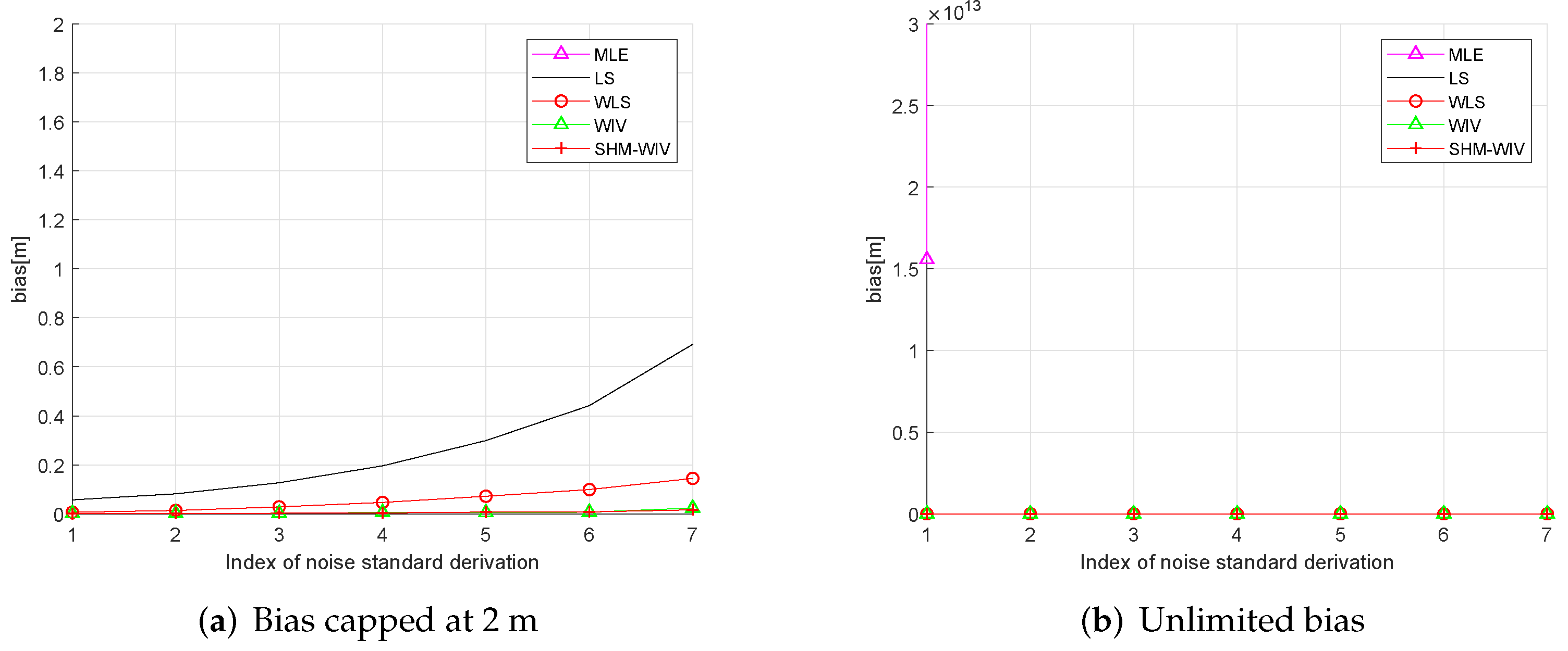
In these simulations 100 source locations are generated randomly in the 60 m × 60 m region, and, for each source location, RMSE and bias are evaluated using 10,000 Monte Carlo runs. The RMSE and bias results are shown in Figure 8 and Figure 9, respectively. The MLE has a divergence problem across the whole noise range. Among the remaining algorithms, the LS has the largest bias and RMSE. The WLS shows improved performance compared to the LS. The WIV and SHM-WIV have the best RMSE and bias performance with the SHM-WIV slightly outperforming the WIV at large noise levels.

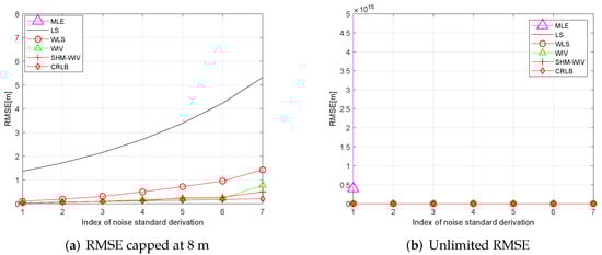
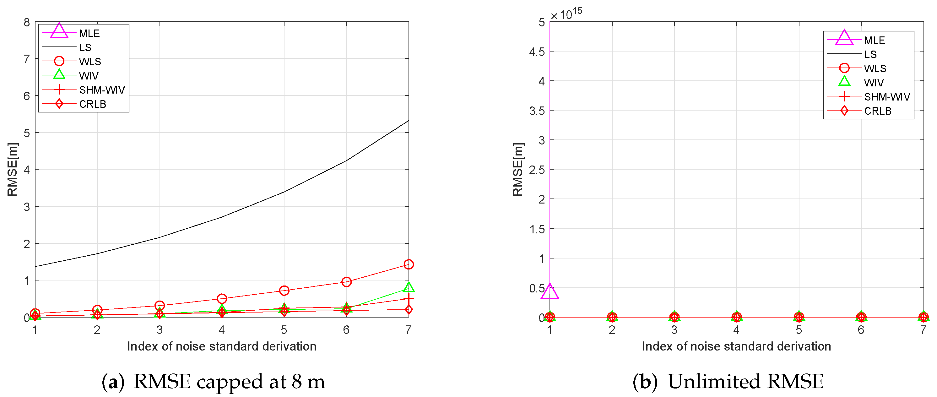
Figure 8. (a) RMSE versus noise with randomized source location (RMSE is capped at 8 m); (b) RMSE versus noise with randomized source location (MLE is missing in (a) as it diverges for entire noise range).

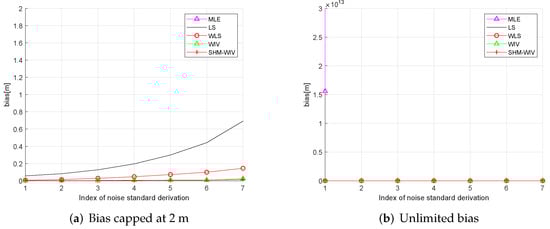
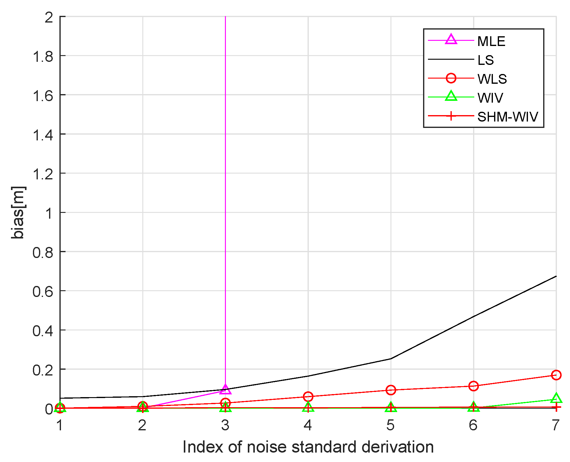
Figure 9. (a) Bias versus noise with randomized source location (bias is capped at 2 m); (b) Bias versus noise with randomized source location (MLE is missing in (a) as it diverges for entire noise range).

7. Conclusions

A new pseudolinear hybrid DRSS-AOA localization method, free of nuisance parameter (squared source range from the reference sensor), was developed by exploiting the geometric relationship between AOA and DRSS measurements. To solve the resulting linear matrix equation for the source location, several variants of the pseudolinear estimator were proposed. These estimators are closed-form, leading to fewer computational steps than the MLE. However, the LS and WLS solutions have severe bias problems as verified by the simulations. The WIV estimator, on the other hand, was seen to be capable of alleviating the bias problem, achieving approximately zero bias for a large number of sensor measurements and small noise. The SHM-WIV was developed to guarantee a strong correlation between the IV matrix and the linearized data matrix for the WIV method as this correlation can be weakened when the noise is large. Simulation studies were carried out to compare the performance of the proposed estimators in fixed and randomized localization geometries. It was observed that the MLE has severe stability issues and cannot be considered an optimal solution at large noise. In the simulation studies the SHM-WIV outperformed all the estimators with an RMSE close to the CRLB and bias approaching zero.

References

- Stansfield, R.G. Statistical theory of d.f. fixing. J. Inst. Electr. Eng. Part IIIA Radiocommun. 1947, 94, 762–770. [Google Scholar] [CrossRef]
- Torrieri, D.J. Statistical Theory of Passive Location Systems. IEEE Trans. Aerosp. Electron. Syst. 1984, AES-20, 183–198. [Google Scholar] [CrossRef] [Green Version]
- Nardone, S.; Lindgren, A.; Gong, K. Fundamental properties and performance of conventional bearings-only target motion analysis. IEEE Trans. Autom. Control 1984, 29, 775–787. [Google Scholar] [CrossRef]
- Ljung, L.; Söderström, T. Theory and Practice of Recursive Identification; MIT Press: Cambridge, MA, USA, 1983. [Google Scholar]
- Athley, F. Threshold region performance of maximum likelihood direction of arrival estimators. IEEE Trans. Signal Process. 2005, 53, 1359–1373. [Google Scholar] [CrossRef]
- Lingren, A.G.; Gong, K.F. Position and velocity estimation via bearing observations. IEEE Trans. Aerosp. Electron. Syst. 1978, AES-14, 564–577. [Google Scholar] [CrossRef]
- Pages-Zamora, A.; Vidal, J.; Brooks, D. Closed-form solution for positioning based on angle of arrival measurements. In Proceedings of the 13th IEEE International Symposium on Personal, Indoor and Mobile Radio Communications, Lisboa, Portugal, 15–18 September 2002; Volume 4, pp. 1522–1526. [Google Scholar] [CrossRef]
- Aidala, V.J.; Nardone, S.C. Biased Estimation Properties of the Pseudolinear Tracking Filter. IEEE Trans. Aerosp. Electron. Syst. 1982, AES-18, 432–441. [Google Scholar] [CrossRef]
- Chan, Y.T.; Rudnicki, S.W. Bearings-only and Doppler-bearing tracking using instrumental variables. IEEE Trans. Aerosp. Electron. Syst. 1992, 28, 1076–1083. [Google Scholar] [CrossRef]
- Holtsberg, A.; Holst, J.H. A nearly unbiased inherently stable bearings-only tracker. IEEE J. Ocean. Eng. 1993, 18, 138–141. [Google Scholar] [CrossRef]
- Pham, D.T. Some quick and efficient methods for bearing-only target motion analysis. IEEE Trans. Signal Process. 1993, 41, 2737–2751. [Google Scholar] [CrossRef]
- Nardone, S.C.; Graham, M.L. A closed-form solution to bearings-only target motion analysis. IEEE J. Ocean. Eng. 1997, 22, 168–178. [Google Scholar] [CrossRef]
- Doğançay, K. Bias compensation for the bearings-only pseudolinear target track estimator. IEEE Trans. Signal Process. 2005, 54, 59–68. [Google Scholar] [CrossRef]
- Ho, K.; Chan, Y. An asymptotically unbiased estimator for bearings-only and Doppler-bearing target motion analysis. IEEE Trans. Signal Process. 2006, 54, 809–822. [Google Scholar] [CrossRef]
- Ho, K.C.; Chan, Y.T. Geometric-Polar Tracking From Bearings-Only and Doppler-Bearing Measurements. IEEE Trans. Signal Process. 2008, 56, 5540–5554. [Google Scholar] [CrossRef]
- Gu, G. A novel power-bearing approach and asymptotically optimum estimator for target motion analysis. IEEE Trans. Signal Process. 2011, 59, 912–922. [Google Scholar] [CrossRef]
- Zhang, Y.; Xu, G.Z. Bearings-only target motion analysis via instrumental variable estimation. IEEE Trans. Signal Process. 2010, 58, 5523–5533. [Google Scholar] [CrossRef]
- Dogancay, K. 3D Pseudolinear Target Motion Analysis From Angle Measurements. IEEE Trans. Signal Process. 2015, 63, 1570–1580. [Google Scholar] [CrossRef]
- Pang, F.; Wen, X. A Novel Closed-Form Estimator for AOA Target Localization Without Prior Knowledge of Noise Variances. Circ. Syst. Signal Process. 2021, 40, 3573–3591. [Google Scholar] [CrossRef]
- Shao, H.J.; Zhang, X.P.; Wang, Z. Efficient Closed-Form Algorithms for AOA Based Self-Localization of Sensor Nodes Using Auxiliary Variables. IEEE Trans. Signal Process. 2014, 62, 2580–2594. [Google Scholar] [CrossRef]
- Dogancay, K. Self-localization from landmark bearings using pseudolinear estimation techniques. IEEE Trans. Aerosp. Electron. Syst. 2014, 50, 2361–2368. [Google Scholar] [CrossRef]
- Lee, J.H.; Buehrer, R.M. Location estimation using differential RSS with spatially correlated shadowing. In Proceedings of the Global Telecommunications Conference, 2009. GLOBECOM 2009, IEEE, Honolulu, HI, USA, 30 November–4 December 2009; pp. 1–6. [Google Scholar]
- Salman, N.; Kemp, A.H.; Ghogho, M. Low complexity joint estimation of location and path-loss exponent. IEEE Wirel. Commun. Lett. 2012, 1, 364–367. [Google Scholar] [CrossRef]
- Hu, Y.; Leus, G. Robust Differential Received Signal Strength-Based Localization. IEEE Trans. Signal Process. 2017, 65, 3261–3276. [Google Scholar] [CrossRef] [Green Version]
- Ogilvy, C.S. Excursions in Geometry; Dover Publications: Mineola, NY, USA, 1990. [Google Scholar]
- Lin, L.; So, H.C.; Chan, Y.T. Accurate and Simple Source Localization Using Differential Received Signal Strength. Digit. Signal Process. 2013, 23, 736–743. [Google Scholar] [CrossRef] [Green Version]
- Sun, Y.; Li, X.; Huang, Z.; Tian, J. An Improved Closed-Form Solution for Differential RSS-based Localization. In Proceedings of the 2020 IEEE Radar Conference (RadarConf20), Florence, Italy, 21–25 September 2020; pp. 1–5. [Google Scholar] [CrossRef]
- Vaghefi, R.M.; Gholami, M.R.; Ström, E.G. RSS-based sensor localization with unknown transmit power. In Proceedings of the 2011 IEEE International Conference on Acoustics, Speech and Signal Processing (ICASSP), Prague, Czech Republic, 22–27 May 2011; pp. 2480–2483. [Google Scholar] [CrossRef] [Green Version]
- Li, J.; Doğançay, K.; Nguyen, N.H.; Law, Y.W. Reducing the bias in DRSS-based localization: An instrumental variable approach. In Proceedings of the 2019 27th European Signal Processing Conference (EUSIPCO), IEEE, Coruña, Spain, 2–6 September 2019; pp. 1–5. [Google Scholar]
- Li, J.; Doğançay, K.; Nguyen, N.H.; Law, Y.W. DRSS-Based Localisation Using Weighted Instrumental Variables and Selective Power Measurement. In Proceedings of the ICASSP 2020—2020 IEEE International Conference on Acoustics, Speech and Signal Processing (ICASSP), IEEE, Barcelona, Spain, 4–8 May 2020; pp. 4876–4880. [Google Scholar]
- Lee, J.H.; Buehrer, R.M. Handbook of Position Location: Theory, Practice, and Advances; Chapter Fundamentals of Received Signal Strength-Based Position Location; Wiley: New York, NY, USA, 2012. [Google Scholar]
- Wang, S.; Jackson, B.R.; Inkol, R. Hybrid RSS/AOA emitter location estimation based on least squares and maximum likelihood criteria. In Proceedings of the 2012 26th Biennial Symposium on Communications (QBSC), IEEE, Kingston, ON, Canada, 28–29 May 2012; pp. 24–29. [Google Scholar]
- Chan, Y.T.; Chan, F.; Read, W.; Jackson, B.R.; Lee, B.H. Hybrid localization of an emitter by combining angle-of-arrival and received signal strength measurements. In Proceedings of the 2014 IEEE 27th Canadian Conference on Electrical and Computer Engineering (CCECE), IEEE, Toronto, ON, Canada, 5–8 May 2014; pp. 1–5. [Google Scholar]
- Tomic, S.; Marikj, M.; Beko, M.; Dinis, R.; Órfão, N. Hybrid RSS-AoA technique for 3-D node localization in wireless sensor networks. In Proceedings of the 2015 International Wireless Communications and Mobile Computing Conference (IWCMC), IEEE, Dubrovnik, Croatia, 24–28 August 2015; pp. 1277–1282. [Google Scholar]
- Tomic, S.; Beko, M.; Dinis, R.; Montezuma, P. A closed-form solution for RSS/AoA target localization by spherical coordinates conversion. IEEE Wirel. Commun. Lett. 2016, 5, 680–683. [Google Scholar] [CrossRef] [Green Version]
- Beko, M.; Tomic, S.; Dinis, R.; Carvalho, P. Apparatus and Method for RSS/AoA Target 3-D Localization in Wireless Networks. U.S. Patent Number 10338193, 2 July 2019. [Google Scholar]
- Nguyen, T.; D Vy, T.; Shin, Y. An efficient hybrid RSS-AoA localization for 3D wireless sensor networks. Sensors 2019, 19, 2121. [Google Scholar] [CrossRef] [PubMed] [Green Version]
- Liu, R.; Wang, D.; Yin, J.; Wu, Y. Constrained total least squares localization using angle of arrival and time difference of arrival measurements in the presence of synchronization clock bias and sensor position errors. Int. J. Distrib. Sens. Networks 2019, 15, 1550147719858591. [Google Scholar] [CrossRef] [Green Version]
- Deng, B.; Sun, Z.B.; He, Q. Efficient closed-form estimator for moving source localization using TDOA-FDOA-AOA measurements. In Proceedings of the 6th International Conference on Information Engineering, Liaoning, China, 17–18 August 2017; p. 20. [Google Scholar]
- Nguyen, N.H.; Doğançay, K. Multistatic pseudolinear target motion analysis using hybrid measurements. Signal Process. 2017, 130, 22–36. [Google Scholar] [CrossRef]
- Costa, M.S.; Tomic, S.; Beko, M. An SOCP Estimator for Hybrid RSS and AOA Target Localization in Sensor Networks. Sensors 2021, 21, 1731. [Google Scholar] [CrossRef]
- Yang, S.; Wang, G.; Hu, Y.; Chen, H. Robust Differential Received Signal Strength Based Localization With Model Parameter Errors. IEEE Signal Process. Lett. 2018, 25, 1740–1744. [Google Scholar] [CrossRef]
- Kay, S.M. Fundamentals of Statistical Signal Processing: Estimation Theory; PTR Prentice-Hall: Englewood Cliffs, NJ, USA, 1993. [Google Scholar]
- Zekavat, R.; Buehrer, R.M. Handbook of Position Location: Theory, Practice and Advances; John Wiley & Sons: Hoboken, NJ, USA, 2011; Volume 27. [Google Scholar]
- Mendel, J.M. Lessons in Estimation Theory for Signal Processing, Communications, and Control; Prentice-Hall: Englewood Cliffs, NJ, USA, 1995. [Google Scholar]
- Ljung, L. System Identification: Theory for The User, 2nd ed.; Prentice-Hall: Saddle River, NJ, USA, 1999. [Google Scholar]
- Doğançay, K. Passive emitter localization using weighted instrumental variables. Signal Process. 2004, 84, 487–497. [Google Scholar] [CrossRef]
- Stoica, P.; Nehorai, A. MUSIC, maximum likelihood, and Cramer-Rao bound. IEEE Trans. Acoust. Speech, Signal Process. 1989, 37, 720–741. [Google Scholar] [CrossRef]
Publisher’s Note: MDPI stays neutral with regard to jurisdictional claims in published maps and institutional affiliations. |
© 2021 by the authors. Licensee MDPI, Basel, Switzerland. This article is an open access article distributed under the terms and conditions of the Creative Commons Attribution (CC BY) license (https://creativecommons.org/licenses/by/4.0/).