
Mobile Computing with a Smart Cricket Ball: Discovery of Novel Performance Parameters and Their Practical Application to Performance Analysis, Advanced Profiling, Talent Identification and Training Interventions of Spin Bowlers


Abstract
1. Introduction
2. Materials and Methods
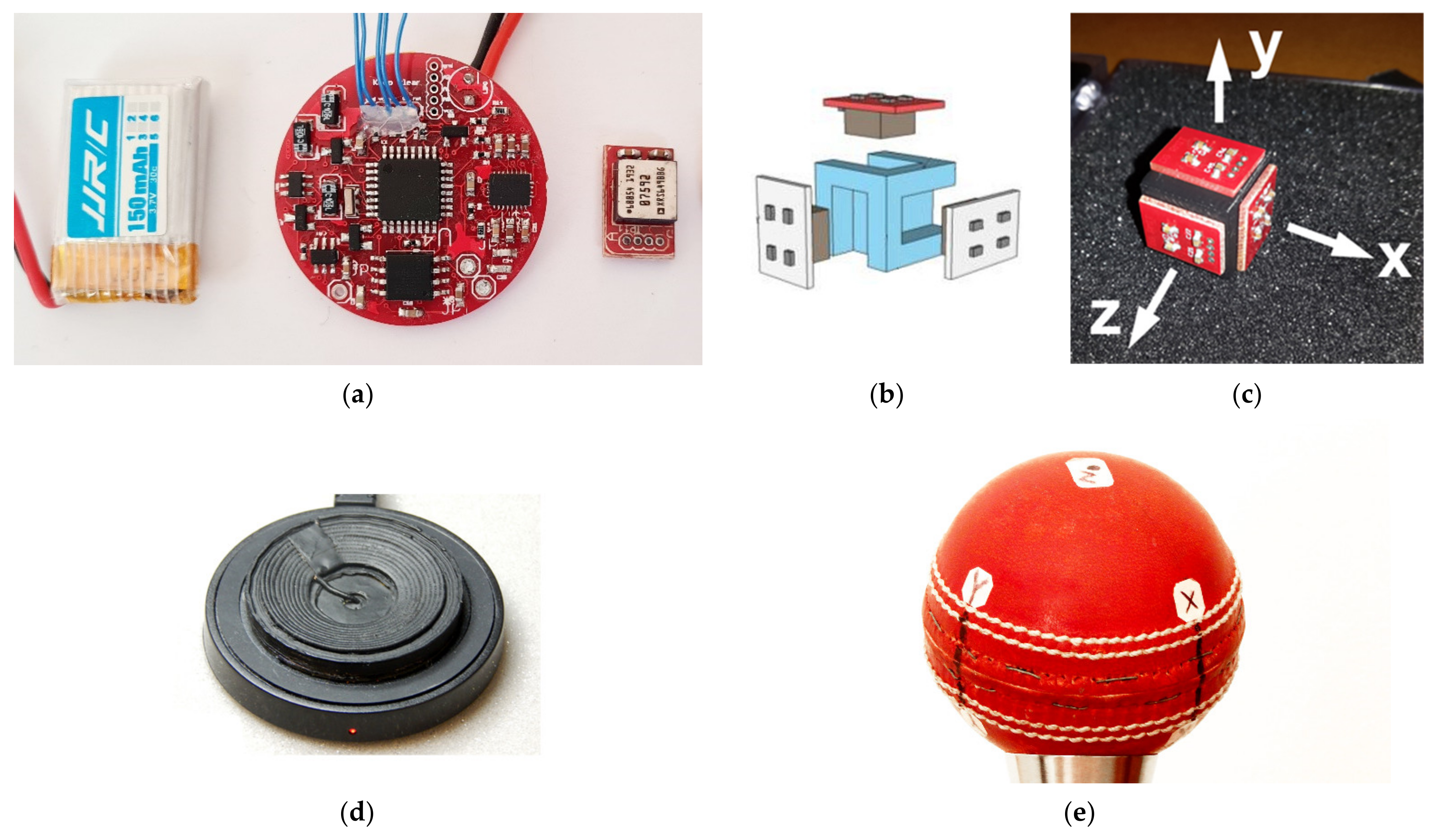
2.1. Development and Specifications of the Smart Cricket Ball
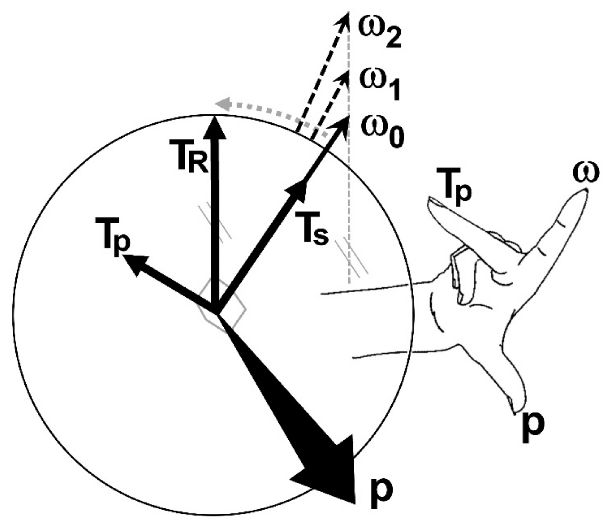
2.2. Performance Parameters
2.3. Applications of the Performance Parameters
2.3.1. Study 1
2.3.2. Study 2
2.3.3. Study 3
2.3.4. Study 4
3. Results
3.1. Study 1
3.2. Study 2
3.3. Study 3
3.4. Study 4
4. Discussion
5. Conclusions
Author Contributions
Funding
Institutional Review Board Statement
Informed Consent Statement
Data Availability Statement
Conflicts of Interest
References
- Wilkins, B. Cricket: The Bowler’s Art; Kangaroo Press: East Roseville, CA, USA, 1997; pp. 69–136. [Google Scholar]
- Woolmer, B.; Noakes, T. Bob Woolmer’s Art and Science of Cricket; New Holland Publishers: London, UK, 2008. [Google Scholar]
- McLeod, P.; Jenkins, S. Timing accuracy and decision time in high speed ball games. Int. J. Sport Psychol. 1991, 22, 279–295. [Google Scholar]
- Beach, A.; Ferdinands, R.; Sinclair, P. Three-dimensional linear and angular kinematics of a spinning cricket ball. Sports Technol. 2014, 7, 12–25. [Google Scholar] [CrossRef]
- Spratford, W.; Whiteside, D.; Elliott, B.; Portus, M.; Brown, N.; Alderson, J. Does performance level affect initial ball flight kinematics in finger and wrist-spin cricket bowlers? J. Sports Sci. 2018, 36, 651–659. [Google Scholar] [CrossRef]
- Abernethy, B.; Russell, D.G. Advanced cue utilisation by skilled cricket batsmen. Aust. J. Sci. Med. Sport 1984, 16, 2–10. [Google Scholar]
- Penrose, J.M.T.; Roach, N.K. Decision making and advanced cue utilisation by cricket batsmen. J. Hum. Mov. Stud. 1995, 29, 199–218. [Google Scholar]
- Renshaw, I.; Fairweather, M.M. Cricket bowling deliveries and the discrimination ability of professional and amateur batters. J. Sports 2000, 18, 951–957. [Google Scholar] [CrossRef]
- Beach, A.; Ferdinands, R.; Sinclair, P. The kinematic differences between off-spin and leg-spin bowling in cricket. Sports Biomech. 2016, 15, 295–313. [Google Scholar] [CrossRef] [PubMed]
- Sanders, L.; Felton, P.J.; King, M.A. Kinematic parameters contributing to the production of spin in elite finger spin bowling. J. Sports Sci. 2018, 36, 2787–2793. [Google Scholar] [CrossRef]
- Fuss, F.K. Instrumentation of Athletes and Equipment during Competitions. Sports Technol. 2008, 1, 235–236. [Google Scholar] [CrossRef]
- Fuss, F.K. Instrumentation of Sports Equipment. In Routledge Handbook of Sports Technology and Engineering; Fuss, F.K., Subic, A., Strangwood, M., Mehta, R., Eds.; Routledge/Taylor & Francis: London, UK, 2014. [Google Scholar]
- Fuss, F.K.; Lythgo, N.; Smith, R.M.; Benson, A.C.; Gordon, B. Identification of key performance parameters during off-spin bowling with a smart cricket ball. Sports Technol. 2011, 4, 159–163. [Google Scholar] [CrossRef]
- Fuss, F.K.; Smith, R.M.; Subic, A. Determination of spin rate and axes with an instrumented cricket ball. Procedia Eng. 2012, 34, 128–133. [Google Scholar] [CrossRef]
- Fuss, F.K.; Smith, R.M. Should the Finger Pressure be Well Distributed Across the Seam in Seam Bowling? A Problem of Precession and Torque. Procedia Eng. 2013, 60, 453–458. [Google Scholar] [CrossRef][Green Version]
- Fuss, F.K.; Smith, R.M. Accuracy performance parameters of seam bowling, measured with a smart cricket ball. Procedia Eng. 2014, 72, 435–440. [Google Scholar] [CrossRef]
- Doljin, B.; Fuss, F.K. Development of a smart cricket ball for advanced performance analysis of bowling. Procedia Technol. 2015, 20, 133–137. [Google Scholar] [CrossRef]
- Fuss, F.K.; Doljin, B.; Ferdinands, R.E.D.; Beach, A. Dynamics of Spin Bowling: The Normalized Precession of the Spin axis Analysed with a Smart Cricket Ball. Procedia Eng. 2015, 112, 196–201. [Google Scholar] [CrossRef][Green Version]
- Fuss, F.K.; Doljin, B.; Ferdinands, R.E.D. Case Studies of the Centre of Pressure Between Hand and Ball in Off-spin Bowling, Analysed with a Smart Cricket Ball. Procedia Eng. 2016, 147, 203–207. [Google Scholar] [CrossRef][Green Version]
- Fuss, F.K.; Doljin, B.; Ferdinands, R.E.D. Effect on Bowling Performance Parameters When Intentionally Increasing the Spin Rate, Analysed with a Smart Cricket Ball. Proceedings 2018, 2, 226. [Google Scholar] [CrossRef]
- Fuss, F.K.; Doljin, B.; Ferdinands, R.E.D. Effect of the Grip Angle on Off-Spin Bowling Performance Parameters, Analysed with a Smart Cricket Ball. Proceedings 2018, 2, 204. [Google Scholar] [CrossRef]
- Fuss, F.K.; Doljin, B.; Ferdinands, R.E.D. Bowling performance assessed with a smart cricket ball: A novel way of profiling bowlers. Proceedings 2020, 49, 141. [Google Scholar] [CrossRef]
- Kookaburra. Smart Ball FAQs. 2021. Available online: https://www.kookaburrasport.com.au/cricket/team-kookaburra/innovation/ (accessed on 5 August 2021).
- Kumar, A.; Espinosa, H.G.; Worsey, M.; Thiel, D.V. Spin Rate Measurements in Cricket Bowling Using Magnetometers. Proceedings 2020, 49, 9011. [Google Scholar] [CrossRef]
- Sportcor. Kookaburra Smartball. 2021. Available online: https://www.sportcor.com/ (accessed on 5 August 2021).
- Williams, A. Smart Cricket Ball measures your bowling performance. Electron. Wkly. 2020, 1. Available online: https://www.electronicsweekly.com/blogs/gadget-master/sensors/smart-cricket-ball-measures-bowling-performance-2020-01/ (accessed on 5 August 2021).
- Mehta, R.D. An overview of cricket ball swing. Sports Eng. 2005, 8, 181–192. [Google Scholar] [CrossRef]
- Mehta, R.D. Sports Ball Aerodynamics. In Sport Aerodynamics; Nørstrud, H., Ed.; Springer: Vienna, Austria, 2008; pp. 229–331. [Google Scholar]
- Geen, J.A.; Kuang, J. Cross-quad and Vertically Coupled Inertial Sensors. U.S. Patent US7421897B2, 9 September 2008. [Google Scholar]
- Weizman, Y.; Tan, A.M.; Fuss, F.K. Measurement of flight dynamics of a Frisbee measured with a triaxial MEMS gyroscope. Proceedings 2020, 49, 66. [Google Scholar] [CrossRef]
- Weldon, A.; Clarke, N.D.; Pote, L.; Bishop, C. Physical profiling of international cricket players: An investigation between bowlers and batters. Biol. Sport 2021, 38, 507–515. [Google Scholar] [CrossRef]
- McGrath, R.E.; Meyer, G.J. When Effect Sizes Disagree: The Case of r and d. Psychol. Methods 2006, 11, 386–401. [Google Scholar] [CrossRef] [PubMed]
- Doljin, B.; Jeong, K.; Kim, Y.-K.; Fuss, F.K. Profiling of a pitcher's performance with a smart baseball: A case report. Proceedings 2020, 49, 103. [Google Scholar] [CrossRef]
- Burnett, A.; Elliott, B.; Marshall, R.N. The effect of a 12-over spell on fast bowling technique in cricket. J. Sports Sci. 1995, 13, 329–341. [Google Scholar] [CrossRef] [PubMed]
- Schaefer, A.; O’Dwyer, N.; Ferdinands, R.E.D.; Edwards, S. Consistency of kinematic and kinetic patterns during a prolonged spell of cricket fast bowling: An exploratory laboratory study. J. Sports Sci. 2018, 36, 679–690. [Google Scholar] [CrossRef]


| Physical Performance Parameters | Training Target | Skill Performance Parameters | Training Target |
|---|---|---|---|
| Maximum spin rate ωR | Improve | Maximum precession p (before the torque spike) | Reduce |
| Maximum angular acceleration α | Improve | Maximum normalised precession pn = θ (before the torque spike) | Reduce |
| Maximum resultant torque TR | Improve | Maximum precession torque Tp | Reduce |
| Maximum spin torque Ts | Improve | Efficiency η | Improve |
| Maximum power P | Improve | ‘Frequency’ αmax/ωmax | Reduce |
| Skill Parameter | Log10pmax | pn_max | Tp_max | η | αmax/ωmax |
|---|---|---|---|---|---|
| F + W + X | 4.25% | 18.63% | 32.29% | 23.19% | 6.66% |
| F + W | 15.18% | 43.69% | 48.51% | 34.69% | 27.47% |
| X | 5.41% | 15.97% | 25.89% | 38.53% | 6.77% |
| Spin Rate ω (rps) | Maximum Precession p (rad/s) | Maximum Normalised Precession pn (deg) | Maximum Resultant Torque TR (Nm) | Maximum Spin Torque Ts (Nm) | Maximum Precession Torque Tp (Nm) | Maximum Power P (W) | Effici-ency η (%) | Ratio αmax/ωmax (s–1) | |
|---|---|---|---|---|---|---|---|---|---|
| 10-over spell, participant 1 (finger-spin topsidespin) | |||||||||
| Mean | 25.95 | 33.40 | 89.29 | 0.2913 | 0.2815 | 0.1142 | 26.83 | 54.76 | 22.20 |
| RMSE | 0.73 | 2.02 | 4.93 | 0.0113 | 0.0101 | 0.0062 | 1.60 | 2.10 | 0.36 |
| RMSE% (= CVRMSD) | 2.81 | 6.04 | 5.56 | 3.88 | 3.90 | 5.46 | 5.97 | 3.83 | 1.63 |
| R2 | 0.0402 | 0.0146 | 0.1522 | 0.0466 | 0.0429 | 0.0293 | 0.0402 | 0.0559 | 0.0233 |
| p-value (alpha = 0.1) | 0.1171 | 0.3510 | 0.0017 | 0.0924 | 0.1062 | 0.1821 | 0.1194 | 0.0650 | 0.2349 |
| Trend of regression | Increase | nil | Increase | Increase | Increase | nil | Increase | Decrease | nil |
| Effect on performance | Gain | nil | Loss | Gain | Gain | nil | Gain | Loss | nil |
| Δ 10-over | 0.50 | 6.95 | 0.0083 | 0.0077 | 1.09 | −1.70 | |||
| %change | 1.91 | 7.79 | 2.85 | 2.74 | 4.06 | −3.11 | |||
| 10-over spell, participant 2 (wrist-spin sidespin) | |||||||||
| Mean | 28.43 | 21.12 | 80.18 | 0.2821 | 0.2238 | 0.1960 | 24.60 | 64.86 | 16.13 |
| RMSE | 1.34 | 3.08 | 14.16 | 0.0213 | 0.0173 | 0.0291 | 2.85 | 4.17 | 1.12 |
| RMSE% (= CVRMSD) | 4.72 | 14.73 | 17.72 | 7.56 | 7.70 | 15.04 | 11.61 | 6.40 | 6.91 |
| R2 | 0.0661 | 0.0495 | 0.0178 | 0.0702 | 0.0828 | 0.0531 | 0.043 | 0.0415 | 0.2058 |
| p-value (alpha = 0.1) | 0.1008 | 0.1576 | 0.4004 | 0.0895 | 0.0647 | 0.1415 | 0.1878 | 0.1943 | 0.0025 |
| Trend of regression | Increase | nil | nil | Increase | Decrease | nil | nil | nil | Decrease |
| Effect on performance | Gain | nil | nil | Gain | Loss | nil | nil | nil | Gain |
| Δ 10-over | 1.75 | 0.0286 | −0.0254 | −2.80 | |||||
| %change | 6.14 | 10.14 | −11.36 | −17.34 | |||||
| 10-over spell, participant 3 (finger-spin topsidespin) | |||||||||
| Mean | 21.23 | 42.35 | 64.55 | 0.2410 | 0.2205 | 0.1200 | 17.75 | 50.92 | 21.22 |
| RMSE | 1.54 | 5.03 | 7.04 | 0.0204 | 0.0221 | 0.0115 | 2.89 | 6.04 | 0.83 |
| RMSE% (= CVRMSD) | 7.22 | 11.89 | 10.91 | 8.47 | 10.01 | 9.54 | 16.18 | 11.91 | 3.91 |
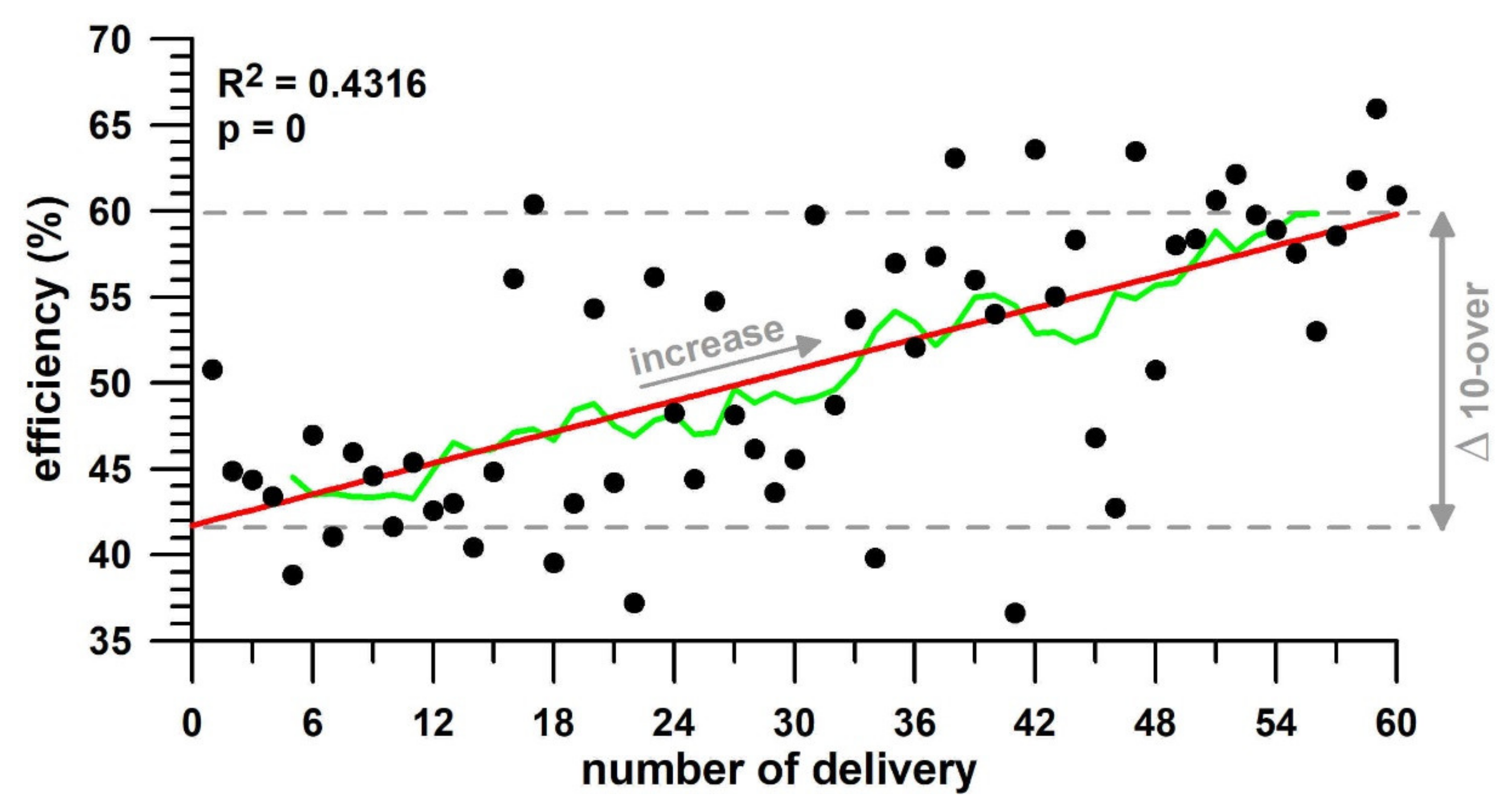
| R2 | 0.0534 | 0.013 | 0.0006 | 0.0459 | 0.0732 | 0.0031 | 0.0508 | 0.4316 | 0.0764 |
| p-value (alpha = 0.1) | 0.0755 | 0.3879 | 0.8500 | 0.1003 | 0.0366 | 0.6760 | 0.0837 | 0.000 | 0.0326 |
| Trend of regression | Decrease | nil | nil | Decrease | Decrease | nil | Decrease | Increase | Decrease |
| Effect on performance | Loss | nil | nil | Loss | Loss | nil | Loss | Gain | Gain |
| Δ 10-over | −1.26 | −0.0154 | −0.0213 | −2.30 | 18.08 | −0.82 | |||
| %change | −5.91 | −6.39 | −9.68 | −12.96 | 35.52 | −3.85 | |||
| Spin Rate ω (rps) | Maximum Precession p (rad/s) | Maximum Normalised Precession pn (deg) | Maximum Resultant Torque TR (Nm) | Maximum Spin Torque Ts (Nm) | Maximum Precession Torque Tp (Nm) | Maximum Angular Acceleration α (rad/s2) | Maxi-mum Power P (W) | Effici-ency η (%) | Ratio αmax / ωmax (s–1) | Minimum Ts (Nm) Before Peak Datum | Average Tp (Nm) of a 0.123 s Window (cf. Figure 10) | |
|---|---|---|---|---|---|---|---|---|---|---|---|---|
| Profiling, before the training intervention | ||||||||||||
| Avg | 28.31 | 40.14 | 94.69 | 0.3309 | 0.3172 | 0.1405 | 4079 | 32.38 | 39.09 | 22.93 | −0.0055 | 0.0428 |
| Std | 0.8 | 2.66 | 8.82 | 0.0112 | 0.0091 | 0.0183 | 117.2 | 1.81 | 4.24 | 0.23 | 0.0104 | 0.0065 |
| Min | 27.18 | 35.01 | 86.91 | 0.3156 | 0.3052 | 0.1143 | 3925 | 30.23 | 34.13 | 22.64 | −0.0223 | 0.0346 |
| Max | 29.23 | 42.51 | 108.51 | 0.3463 | 0.3307 | 0.1601 | 4253 | 34.94 | 45.75 | 23.2 | 0.0033 | 0.0492 |
| After the training intervention | ||||||||||||
| Avg | 24.97 | 38.3 | 78.26 | 0.2781 | 0.2674 | 0.1234 | 3439 | 24.66 | 58.83 | 21.91 | 0.0092 | 0.027 |
| Std | 0.78 | 2.19 | 6.07 | 0.0107 | 0.0111 | 0.0081 | 143.3 | 1.71 | 1.75 | 0.33 | 0.0042 | 0.0032 |
| Min | 23.8 | 34.54 | 71.53 | 0.2603 | 0.2488 | 0.1106 | 3200 | 21.96 | 57.02 | 21.4 | 0.0006 | 0.022 |
| Max | 25.84 | 40.95 | 89.45 | 0.2911 | 0.2816 | 0.1333 | 3622 | 26.41 | 61.12 | 22.47 | 0.0134 | 0.0307 |
| After several days of self-training | ||||||||||||
| Avg | 27.59 | 38.33 | 90.39 | 0.3197 | 0.3058 | 0.1339 | 3932 | 30.76 | 55.2 | 22.68 | −0.0003 | 0.0296 |
| Std | 0.73 | 1.08 | 4.47 | 0.0139 | 0.014 | 0.0027 | 179.9 | 1.82 | 2.07 | 0.45 | 0.0042 | 0.0015 |
| Min | 26.2 | 36.58 | 85.12 | 0.2953 | 0.2806 | 0.1298 | 3608 | 27.4 | 52.12 | 21.92 | −0.0055 | 0.0269 |
| Max | 28.38 | 39.49 | 96.3 | 0.3386 | 0.324 | 0.1379 | 4167 | 33.04 | 58.79 | 23.36 | 0.005 | 0.0309 |
Publisher’s Note: MDPI stays neutral with regard to jurisdictional claims in published maps and institutional affiliations. |
© 2021 by the authors. Licensee MDPI, Basel, Switzerland. This article is an open access article distributed under the terms and conditions of the Creative Commons Attribution (CC BY) license (https://creativecommons.org/licenses/by/4.0/).
Share and Cite
Fuss, F.K.; Doljin, B.; Ferdinands, R.E.D. Mobile Computing with a Smart Cricket Ball: Discovery of Novel Performance Parameters and Their Practical Application to Performance Analysis, Advanced Profiling, Talent Identification and Training Interventions of Spin Bowlers. Sensors 2021, 21, 6942. https://doi.org/10.3390/s21206942
Fuss FK, Doljin B, Ferdinands RED. Mobile Computing with a Smart Cricket Ball: Discovery of Novel Performance Parameters and Their Practical Application to Performance Analysis, Advanced Profiling, Talent Identification and Training Interventions of Spin Bowlers. Sensors. 2021; 21(20):6942. https://doi.org/10.3390/s21206942
Chicago/Turabian StyleFuss, Franz Konstantin, Batdelger Doljin, and René E. D. Ferdinands. 2021. "Mobile Computing with a Smart Cricket Ball: Discovery of Novel Performance Parameters and Their Practical Application to Performance Analysis, Advanced Profiling, Talent Identification and Training Interventions of Spin Bowlers" Sensors 21, no. 20: 6942. https://doi.org/10.3390/s21206942
APA StyleFuss, F. K., Doljin, B., & Ferdinands, R. E. D. (2021). Mobile Computing with a Smart Cricket Ball: Discovery of Novel Performance Parameters and Their Practical Application to Performance Analysis, Advanced Profiling, Talent Identification and Training Interventions of Spin Bowlers. Sensors, 21(20), 6942. https://doi.org/10.3390/s21206942