1. Introduction
Radars with large uniformly distributed array antennas have been widely applied in atmosphere observation [
1], military warning, and navigation [
2] with an increasing speed. To reduce the kind of the Transmitting/Receiving (T/R) modules to simplify the transmitting feeding network in array antennas as well as to suppress the MSLL as much as possible, several design ideas are presented. First is the thinned arrays. In the previous stage, Willey [
3] and Skolnik [
4] investigated the density-weighted thinned arrays. Soon afterward, nature-inspired algorithms such as genetic search [
5,
6] and particle swarm optimization [
7] have been exploited to design thinned arrays. However, due to the very intensive computational efforts, those stochastic optimization-based methods are not suited for large array thinning [
8]. Later on, the Iterative Fourier Technique (IFT) [
8] as well as its derived IFT-based algorithms [
9,
10] and more recent dynamic programming [
11] have been successfully applied to large array thinning. Another solution is the nonuniformly distributed arrays, e.g., [
12,
13,
14,
15,
16]. Though they may outperform thinned arrays in many aspects theoretically, the interelement spacing is changed, which violates the nature of the uniform distribution.
From the form of excitation coefficients, thinned arrays are two-step [0, 1] quantized weights arrays, and the amplitude coefficients at elements that remained are equal. The primary motivation of array thinning is the reduction in cost and weight. At the same time, a low MSLL can be obtained without evidently widening the Half-Power BeamWidth (HPBW) if the amplitude distributions are properly configured [
8]. Though the reported lowest MSLL of thinned arrays has been improved many times, however, the lowest attainable MSLL associates with the number of antennas, when the total number of elements is not large, the MSLL is not low [
17]. To further suppress the MSLL without increasing the number of elements, the concept of quantized weights arrays is introduced. Essentially, the distribution generated by quantized weights is a combination of density and amplitude tapering, which further smooths the average amplitude illumination [
18]. However, the quantized weights arrays require a set of discrete amplitude weights. Whether the weight set is provided in advance or generated simultaneously during the synthesizing process, extra optimization dimensions are added, thus directly increasing the complexity of solving the problem. In addition, varied methods applied well for synthesizing classical two-step thinned arrays are not applicable here to synthesize quantized weights arrays. Therefore, it is relatively more difficult to synthesize perfect quantized weights arrays.
Till now, only a few studies have addressed this topic [
17,
19,
20,
21,
22,
23]. Even so, they are all implemented in a very similar statistical way. Ball [
20] designed several sets of quantized weights and concluded that the set wherein the weights are equally spaced and distributed between zero, and one can obtain one of the largest reductions in MSLL when the selection probabilities are the terms of the binomial distribution. Gao [
17] calculated the optimum quantized weights from a nonlinear optimization problem which minimizes the variance between the reference pattern and the synthesized pattern. Except for those, the other used quantized weights are generated randomly [
21] or preset with several specific particular values [
19,
22], which may be far from the global optimum. Li [
24] summarized the relationship between the quantized amplitudes arrays with the statistical density tapering arrays and concluded that the latter is only a special form of the former, but the proposed method to design quantized amplitude arrays is essentially the same as that of in [
17]. More recently, Shao [
22] added some modifications to [
21] and found that lower MSLL can be obtained when the illumination probability of one element is also relevant to the illumination probabilities of other elements in the adjacent positions. The performance of [
22] is better than that of [
21] in some situations but still worse than that of [
17].
Except for some theoretical studies mentioned above, quantized weights arrays have been applied to several Very High Frequency (VHF) radars for the observation of neutral atmosphere and Field Aligned Irregularities (FAIs). Unlike the turbulence echo in the neutral atmosphere, the FAIs are also very sensitive to the weak radio frequency signals. In some ionospheric strong scattering events, part of the radar echo may be received by the sidelobes [
25]. In this case, the range-time-intensity plot displays the combination of the mainlobe and the sidelobe echoes, which leads to the misjudgment of the actual height and angle of arrival of the FAI echoes. Though the use of the multichannel Spatial Domain Interferometer (SDI) technique can sometimes well reconstruct the actual position of FAIs in space [
26]. However, for a routine-operated VHF radar (requiring a long-time operation) to ensure the quality of the data transmission, the number of consecutive pulses in each data block is quite limited. At this time, the SDI performs badly. Therefore, the most reasonable way is to suppress the MSLL of the transmitting beam. As a consequence, some researchers have developed multiple equivalent approaches to meet the lowest SLL requirements. The stationary SOUSY enlarged the interelement spacing at the edge of the array and fed the antennas at the inner positions with higher power [
27] simultaneously. The mobile SOUSY adopted a three-level power configuration of [1, 0.5, 0.25] to smooth the current distribution at the transmitting stage [
27]. Later, to suppress the MSLL, numerous T/R modules with different powers are adopted in the Indian MST radar to achieve a modified Taylor weighting in both principal directions [
28]. Soon, the new Qinzhou MST radar will also consider the quantized weights to guarantee the transmitting beam with a low MSLL [
1].
Though the use of quantized weights arrays can be traced back to a very early age, there are still some drawbacks, and there has been no evident progress for a long time. One limitation of the previously reported methods is that it is difficult to select an appropriate reference distribution associated with the lowest MSLL because the selected reference distribution does not show any regularities. Another limitation is that the reported methods cannot achieve a notable and stable MSLL attenuation because there is not a solid theoretical foundation, and final results depend largely on probability. In addition, few studies have found further research on this topic in recent years. The purpose of this paper is to further suppress the MSLL of aperture-limited circular arrays with limited quantized weights as well as to push this work forward. We applied a totally new idea to solve this problem and proposed a new method. The idea was inspired by a synthesis problem of concentric ring arrays. To obtain low MSLL, Milligan [
29] developed a technique to design concentric ring arrays. The radius of each ring is specified by dividing the cumulative distribution by the number of rings. Afterward, Bucci [
30] exploited an efficient deterministic method for fast-design high-directivity focusing aperiodic concentric ring arrays with multiple constraints along with the increasing demand in satellite applications. This method establishes a generalized analytical equation between the reference array and the synthesized array, revealing that minimizing the weighted mean square error between the reference pattern and the synthesized pattern is equivalent to minimizing the mean square error between the radial cumulative distributions of the reference distribution and the synthesized distribution. A similar approach is also seen in [
31]. However, using this kind of method associated with radial cumulative distribution to design aperiodic concentric ring arrays, the pattern consistency of reference array and synthesized array only maintains well at near in sidelobes but not the far ones. Usually, an element pattern is needed to lower the level of the far outside lobes [
30].
In this paper, we extend the use of the analytical equation in [
30] for synthesizing uniformly distributed circular arrays with quantized weights and low MSLL. Compared with the previously reported methods, the proposed method not only improves the MSLL performance by about 1–2 dB but also obtains the best results of HPBW and array directivity in all test cases with different apertures, which sheds new light on this topic and presents the significance of the proposed work. We organize this paper as follows: In
Section 2, we first extend the basic theory [
30,
31,
32] of connecting the patterns and distributions to uniformly distributed circular arrays. In
Section 3, we present the proposed method in detail. Various numerical examples and comparisons with several reported statistical methods in terms of the lowest MSLL are given in
Section 4, and
Section 5 concludes this paper.
2. Discussion of the Generalized Relationship Applied for Uniformly Distributed Circular Arrays
For a continuous circular symmetric aperture distribution, the radiation pattern can be expressed as
where
is the zero-order Bessel function of first kind,
R is the radius of the circular aperture, and
is the normalized amplitude.
with
being the wavelength.
with
being the angle measured from the boresight.
For uniformly distributed circular arrays, the circular-shaped aperture can be truncated from the square aperture. To preserve some symmetry in the final layout, we assume that one element is exactly at the center of the circular region. Seen from the center element, the array factor of uniformly distributed arrays can be expressed as
where
N denotes the total number of the array and
is the azimuth angle describing the field.
and
represent the illumination and the azimuth of the
nth element, respectively.
is the distance between the center element and the
nth element.
Dividing the whole array by a sequence of equal-width concentric rings, then the array factor (
2) can be rewritten as a double summation form
where
is the total number of rings and
is the number of element of the
kth ring array. Let the width of the concentric rings to a very small value and discard the rings that do not contain any elements; then, in each remained ring, we have
where
is the number of rings that contain elements. (
4) presents that all the radii
in the
kth ring can be replaced by their mean value
and the total number of rings reduce to
. Then, (
3) simplifies to
We can see that (
5) describes the array factor of the uniformly distributed circular array in a way similar to the concentric ring array. Introducing the discrete array illumination function in the
plane
and using the Jacobi–Anger expansion
(
5) can be transformed into
where there only remains the zero harmonic for the Bessel functions of the first kind go rapidly to zero when the argument
is smaller than the nonzero order, and we focus more on the near-in zenith range
. Moreover, we can find once the nonzero harmonics are dropped, the array factor
is approximated by an azimuth-independent form
. Introducing the average radial ring distribution neglecting the azimuthally asymmetric property
and the radial cumulative function
and combining (
1), (
8)–(
10) we have [
30,
31]
or applying the Parseval’s theorem [
30]
provided that the total distributions of reference array and synthesized array are equal
where
and
represent the radial cumulative function of the reference distribution and the synthesized distribution, respectively.
3. The Proposed Method
Equation (
12) has been applied to the synthesis of large concentric ring arrays. In previous work [
30], the embedded elements are excited with equal illumination, while the element positions are progressively determined. In this paper, the configuration of the elements is determined in advance. To have a better comparison with the reported work [
17,
21,
22], the used arrays are uniformly distributed circular arrays where elements are arranged into an equilateral square grid with
spacing. The primary motivation of applying quantized weights is to suppress the MSLL. Then, if a quantized weights set containing
quantized weights is given as
the optimization problem becomes to minimize the MSLL of the synthesized pattern by determining the amplitude at each element that is subject to a constraint that the amplitude should be in the quantized weights set
. Then, the problem can be formulated as
where
N is the total number of the array.
is the MSLL of the synthesized array applying the aperture distribution
. While the used arrays are uniformly distributed, we can fast calculate the array factor through the inverse Fast Fourier Transform (FFT) [
8]. Additionally, the interelement spacing of
ensures that no grating lobes move into the visible space along with the scanning of the main beam. Then, the MSLL can be regarded as the second maxima in the normalized
plane with
and
. Note in this way that both the visible and invisible space are considered when calculating the MSLL. The optimization problem (
15) is the general form for synthesizing quantized weights arrays with the lowest MSLL. Moreover, considering the practical realization and reducing the complexity of the feed network as much as possible, the normalized quantized weights set
in descending order and adopted in this paper are preset as
. This amplitude configuration is easy to achieve compared to that in [
17] or a sequence of randomly generated weights [
21], benefited from the developed Direct Digital frequency Synthesizer (DDS) technique, and we can control the RF power by adjusting the generated power of DDS. All T/R modules only need to work within the saturation amplification region.
The followed subsections present the basic idea of the approach on how to assign the quantized weights into the aperture distribution in detail.
3.1. Determine the Amplitude Distribution in Each Ring
Since we have known the quantized weights
, the subsequent procedures can be performed similarly to [
9,
11,
32]. We first divide the whole circular aperture by
concentric circle, with
being defined as
where
represents the ceiling function. The radii vector of all the circles are
with
being the radius of the outermost circle, which equals the aperture radius
R. Note that the whole aperture is divided into one circle array and
ring arrays. For convenience, all the subarrays are referred to as ring arrays. The followed procedures start at the innermost subarray, and we radially and progressively assign the quantized weights into the synthesized array by approximating the cumulative function of the reference distribution and the synthesized distribution.
There are two criteria before we put the quantized weights into the synthesized array. The most fundamental criterion is that we should try our best to minimize the mean square error of the radial cumulative distribution between the reference distribution and the synthesized distribution within each circle. Another criterion comes from the consideration of (
9). To ensure that the amplitudes in each ring are azimuthal symmetric, the selected quantized weights in each ring should be as close as possible and the types of weights should be as few as possible. Therefore, there should be at most two types of weight in each ring, and the two weights should be adjacent in the quantized weights set
. Based on this premise, the most suitable weights and the corresponding numbers in the
kth ring can be calculated from an optimization problem specified by
where
is the number of element in the
kth ring.
and
are the numbers of weight
and weight
in the
kth ring.
is the cumulative distribution of the synthesized distribution within the radius
, and
is the cumulative distribution of the reference distribution within the radius
. Note in the first ring, namely
,
equals zero. (
17) can be effectively solved from a for-loop, and the subproblem in each for-loop is a typical convex optimization problem.
3.2. Place the Quantized Weights to the Ring
Once the most suitable weights and the corresponding numbers in one ring are calculated, the subsequent step is to assign the weights into the elements of the ring reasonably. Considering the premise of (
4), the fundamental theoretical derivation weakens the concept of the ring. We emphasize more the sum of the distribution in a narrow ring within a certain radius range. On the other hand, to prevent adverse clustering that further deteriorates the azimuthal symmetric property, the most reasonable way is to space the weights uniformly in the ring [
11]. Then, the problem becomes how to space (at most) two kinds of weights into a ring and make the ring satisfy the rotational symmetry property as much as possible. The simplest situation is that there is only one kind of weight to assign, and what we only need is just to assign it to each element in the ring. When there are two kinds of weights in a ring, to ensure the rotational symmetry of the whole ring as much as possible, it can be equivalent to keeping the rotational symmetry of the elements with the same weight in the ring as much as possible. Since the type of weights in one ring is at most two, and the array elements in the ring are divided into two parts according to the weights, i.e., in the
kth ring, and the number of elements in these two parts are
and
and
. Define
Then, we only need to ensure these
elements satisfy the rotational symmetry as much as possible. One modification is applied before we finally start the synthesis. Considering some bad distributions, namely,
equals one or two, we replace it with zero or three depending on the requirements of (
17) to make it meet (
9) as much as possible. Therefore, the number of any kind of weights in one ring should be greater than or equal to three if there are two kinds of weights in that ring.
In addition, it is worth noting that when dividing the whole circular aperture, we only restrict that the elements in each ring do not overlap in the azimuth. However, we do not guarantee that the distances between the elements and the central element are equal and do not guarantee that the elements in one ring have strict azimuth angular periodicity. The above requirements are not completely satisfied even when the ring width
is narrow enough. Additionally, when the ring width is quite narrow, the number of elements in each ring is very small, which frequently leads to an extremely nonuniform distribution of the weights. For example, the number of one weight in one ring is only one or two. Moreover, though (
4) and (
5) suggest that a narrow ring width is recommended. However, after several tests, we notice that when the elements in one ring are not overlapped in azimuth, the final MSLL suppression is not improved with the further decreasing of the width of each ring. To better take into account this contradiction, we take the ring width as half the element spacing (
) and assume that elements in one ring are equidistant from the center element.
Based on the foregoing presupposition, the initial selection for the
elements can be obtained from a simple procedure.
Figure 1 shows two situations of trying the best to make the
elements satisfy the rotational symmetry, and the details are described in the caption. The advantage of selecting the elements here in this way is that the elements are not required to be uniformly distributed in the azimuth, and we still can select them out appropriately. The introduction of the random offset vector
is to avoid the adverse clustering of elements at the azimuth of 0, because in all situations, the azimuth of the red line within the two purple dotted lines starts at the azimuth of 0. On the other hand, the structure of the red lines is strictly azimuthal symmetric; therefore, the random value in any ring, such as in the
kth ring,
can be limited valued within the range of 0 and
to decrease the search space.
3.3. Refinement
Since a rough quantized weights array can be designed through the previous steps, we can still improve the MSLL performance by a local optimization method. In the previous sections, the offset vector
is generated randomly, and it is difficult to achieve global optimum or even local optimum. One possible way is to calculate the optimal
directly based on some constraints, but the possibility is strongly limited by the problem size [
30]. Therefore, it is unrealistic to optimize the
from a global perspective. Inspired from the refinement method mentioned in [
11], we propose a local optimization method to optimize the
. The process starts at the innermost ring, in each iteration; we only optimize one element of the
; for the
jth iteration, the optimal
takes the value of the followed optimization problem
where
k indicates the corresponding index of the ring started at the innermost ring. The iteration number
j and the ring index
k have the following relationship:
We updated one by one along with increasing the number of iterations. To simplify the process, we skipped the iteration if there is only one kind of weight in the corresponding ring, because in this case, whatever value the takes, it does not affect the final array layout. The synthesis terminates once the MSLL has not changed in iterations or the maximum number of iterations is reached.
Just like (
17), the realization of (
19) can also be achieved through a for-loop. We can discretize the constrained region
with sufficient dense points. Usually, multiple adjacent points lead to the same situation, and we only need to calculate the MSLL of the same situation once. Thus, the computing time is greatly reduced.
3.4. Implementation of the Proposed Method
After much discussion of the details, the proposed method in a single trial can be summarized as follows:
- 1
Initialize the circular aperture array with specified radius R and interelement spacing d from a uniformly distributed square array.
- 2
Choose a suitable reference distribution for the synthesized array.
- 3
Calculate the amplitude distribution in each ring sequentially.
- 4
Place the amplitudes to the ring sequentially.
- 5
Initialize the synthesized array with ten different and keep the case with the lowest MSLL.
- 6
Employ the refinement process to the remained initial array until the termination conditions are met.
A workflow for illustrating the implementation of the proposed method can refer to
Figure 2.
4. Numerical Analysis
In this section, we display some typical results generated by the proposed methods and present some comparisons with the reported statistical methods [
17,
21,
22]. The used arrays are circular planar arrays with diameters of
,
, and
. The element spacing is
, and the width of the ring is
for all considered arrays. The proposed method is capable of synthesizing an array with an unlimited number of quantized weights, and in this paper, we only consider the cases with a number of quantized weights of four. Similar to the reported literature [
21], the mutual coupling between the elements of the array is not considered in this paper.
4.1. Numerical Examples
The reference distribution applied for the proposed method are circular Taylor aperture distributions [
33]. Though the circular Taylor distributions are not applicable in some special circumstances, such as facing an incomplete aperture or an oversized interelement spacing [
34]. However, in this topic, the arrays we use are uniformly distributed arrays with reasonable interelement spacing, and the sampled results are acceptable.
We first apply the proposed method to a circular array with a diameter of
in 20 independent trials. Different circular Taylor aperture distributions with SLL range from −36 to −39 dB in a step of −1 dB and
(number of equal amplitude sidelobes adjacent to the main beam) ranging from 5 to 25 in a step of 5 are used as reference distributions, respectively.
Figure 3 displays the convergence curves of the MSLL as a function of the iteration number during the refinement process of all the trials except the cases with a
of 25, because the corresponding performances are quite bad compared to other cases, and to make the figure clearer, we omit this part in the figure. Two conclusions can be drawn from
Figure 3. First, the MSLL is heavily dependent on the selected reference distribution, and different selections of reference distribution may lead to an MSLL difference of over 2 dB. Second,
seems to play a more important role in final MSLL suppression when
is larger than 10—the smaller the
, the faster the MSLL converges. When
is smaller than 10, the convergence curves are jointly controlled by the SLL and
. The case when the SLL equals −37 dB and
equals 10 reaches the lowest MSLL.
Figure 4 displays the amplitude distribution of the synthesized quantized weights array with the lowest MSLL. The diameter is
, and the number of quantized weights is four. The four quantized weights are [1, 0.50, 0.25, 0], respectively. The MSLL in the whole
plane is equal to
dB.
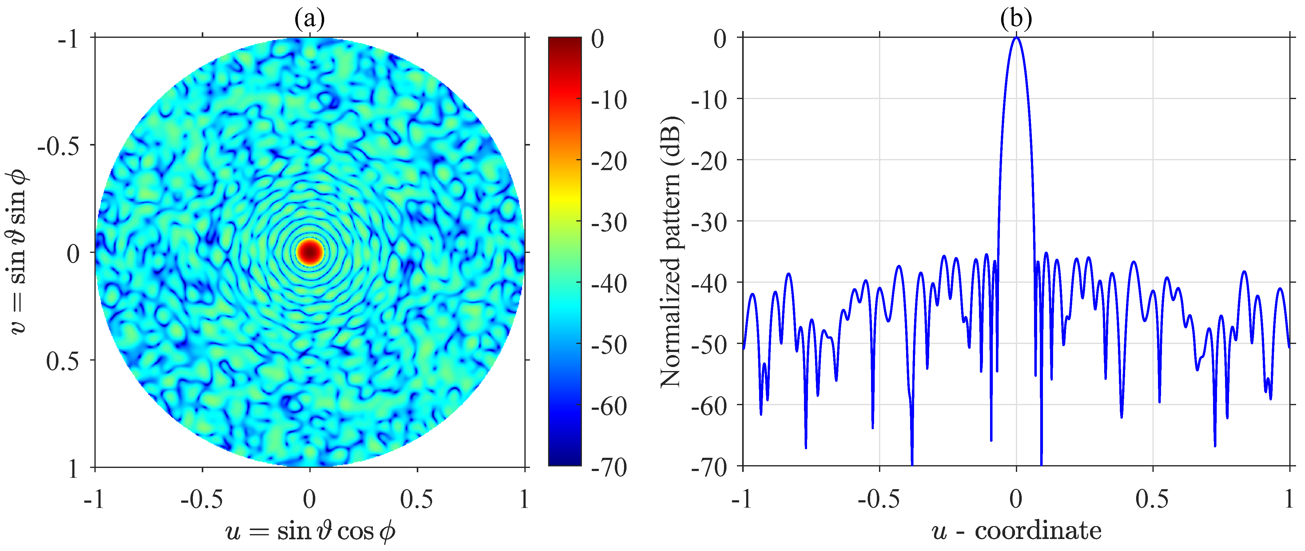
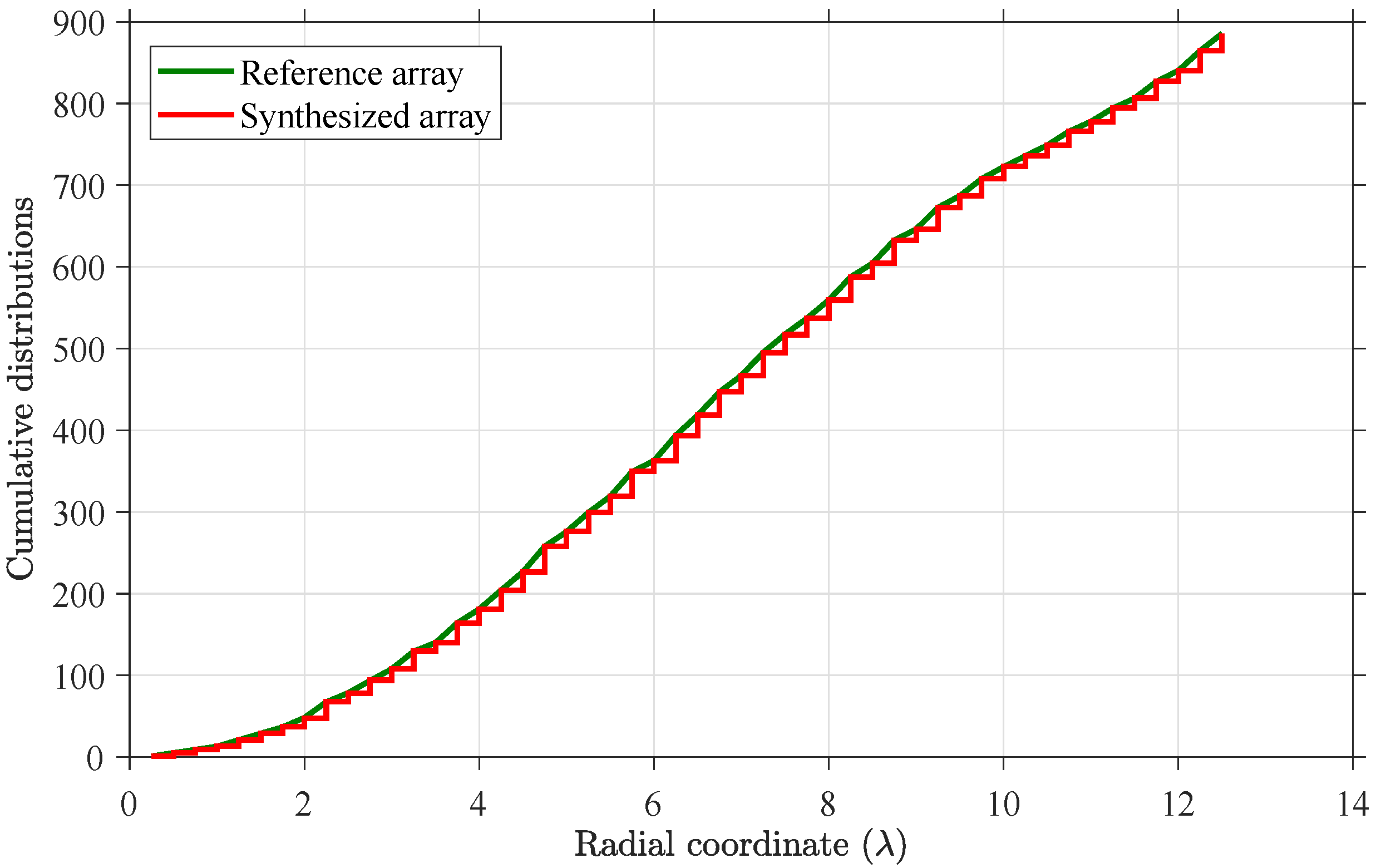
Figure 5 displays the surface plot of two-dimensional radiation pattern and the
u-cut plot of the farfield pattern of the array in
Figure 4. From
Figure 5, we can notice that the first few sidelobes approximate to
dB, and the first few ring-shaped sidelobes near the mainlobe show a circular Taylor-liked pattern because the radial cumulative distributions of reference array and synthesized array presented in
Figure 6 coincide well with each other.
The same experiments but for different reference distributions are also carried out for circular arrays with a diameter of and , both in 20 independent trials. The used SLL of circular Taylor aperture distribution range from −37 to −40 dB and from −41 to −44 dB, both in a step of −1 dB. The used range from 5 to 25 in a step of 5 in all cases. Similar conclusions can also be perceived from the synthesis results. To evaluate the performance of the proposed method, in the next subsection, we present the comparison results between the proposed method and several reported statistical methods.
4.2. Comparisons with the Reported Methods
Table 1 summarizes the synthesis results obtained by the proposed method with the lowest MSLL and several reported statistical methods abbreviated as STAT1 [
21], STAT2 [
17] and ISTAT [
22] for circular aperture arrays with diameters of
,
, and
. Four quantized weights are adopted in all cases. There are three types of quantized weights, which are denoted as
Fixed,
Random, and
Optimized. The proposed method uses the fixed weights type of [1, 0.5, 0.25, 0], and for a more complete comparison, we also carry the experiments with fixed weights using the STAT and ISTAT. While in the original literature, random weights corresponding to the lowest MSLL are adopted. We also list the experiment results with random weights in
Table 1. Unlike other methods, the quantized weights applied in STAT2 are optimized from a nonlinear optimization problem. To have a valid comparison, circular Taylor aperture distribution [
4] with SLL ranging from −35 to −60 dB in a step of −1 dB and
ranging from 6 to 15 in a step of 1 are applied here for the three statistical methods as the reference distributions. For each distribution, we repeat the experiments 10 times. Thus, each listed result of the three statistical methods is the best outcome in terms of the lowest MSLL in 2600 independent trials. This is also the reason why the adopted reference circular Taylor aperture distributions are different, because the lowest MSLL may correspond to different distribution.
In addition, some modifications are introduced. On the one hand, only the cases analogical to “natural thinning” [
4,
21] are considered in this paper. On the other hand, in [
21], three methods were proposed for designing quantized weights arrays. However, after several trials, we find that nearly in all cases in terms of the lowest MSLL, method 2 obtains better results than method 1 and obtains similar results to those of method 3. Therefore, we only display the results obtained by method 2. Moreover, the ISTAT method in [
22] was applied to method 1 of the three methods introduced in [
21]. For better results, we also change it to method 2 and reformulate the iteration equations as follows:
where
is the amplitude of the
nth element when the planar reference distribution is expanded to the line array.
is the density distribution function, and
is the quantized weight assigned to the
nth element.
and
are the indices of the element in quantized weights set
, which are subject to the constraints of
and
.
From
Table 1, it can be noted that in all cases, STAT2 obtains lower MSLL than STAT1 and ISTAT, and all MSLL obtained by the proposed method are lower than those obtained by the three statistical methods. Farfield properties including array directivity and HPBW are also presented. The equation for calculating
is expressed as [
35]
where the main beam points to
. In this paper, we let
and
. Moreover, to ensure a good numerical accuracy for the calculation of HPBW, we interpolate the original
u-cut plot data from 1025 to 10,001 points. We can notice that in all cases in
Table 1, the proposed method can achieve the narrowest HPBW and the largest array directivity compared to all reported statistical methods.
As to a deeper study of the
parameter, other conclusions regarding the HPBW and directivity can be obtained from studying the synthesis results of the circular array with a diameter of
via the proposed method. The HPBW shows a high relationship with the reference taper, which presents an evident negative correlation to the SLL and
. The array directivity does not show an evident relationship to SLL but seems to be related to
. For fair comparison issues, in
Table 2, we also give the results of the number of the array elements that are “ON” (i.e., with a weight different from 0) of the variety of the methods, and we can notice that the proposed method tends to have a larger fill factor. Further discussions about these issues will be given in a future work.
4.3. Discussion of the Proposed Method
Unlike the traditional two-value array thinning, the synthesis problems for quantized weights array are more open. In the proposed method, the final MSLL is associated with multiple variables, including the quantized weights, the reference distribution, the width of the ring sector, and the initial for refinement. In this paper, the dimension of the problem can be reduced through some subjective treatments. Considering the realization, we select a fixed sequence as the quantized weights. As to the ring width, we set it as , because a smaller value does not influence the final results once the elements in one ring are not overlapped in azimuth.
The essence of the proposed method is to approximate the near-in sidelobes of the reference pattern. Thus, it is unlike the reference taper selection strategy revealed in the three reported statistical methods, in which the selected reference distribution does not show any regularities. While the synthesis results show that the SLL of the reference pattern for the proposed method is 3–4 dB lower than the infimum of the MSLL of the array, the infimum of MSLL can refer to the results of the statistical methods. On the other hand, a smaller (≤10) is suggested to ensure a lower MSLL. In addition, the refinement method is not a global optimization method, and only a very limited MSLL suppression of about 2 to 3 dB can be achieved. Therefore, we try to start the refinement process at a low MSLL state as much as possible, and this is the reason why we initialize the for 10 times and select the case with the lowest MSLL before starting the refinement process.
Except for the proposed method, the STAT2 with optimized quantized weights achieve the lowest MSLL, but concerning the other two properties, i.e., maximum directivity and HPBW, the STAT2 does not show any advantage. Moreover, the calculated optimized quantized weights of the STAT2 are hard to practically implement, compared to the fixed-type weights. Thus, in terms of practicability, the proposed method is better.
One evident defect of the proposed method is the required computational time. As shown in the rightmost column of the legend in
Figure 3, the simulation time for most cases with a diameter of
is close to half an hour. For cases with larger diameters, the computational time is presented in
Table 3. We can notice that the computational time increases exponentially with the increases in aperture. To solve this problem, we can adopt a multiple-process approach, where different reference distributions are assigned to different processors. In this way, a very significant time reduction can be achieved.


