
HARNAS: Human Activity Recognition Based on Automatic Neural Architecture Search Using Evolutionary Algorithms


Abstract
:1. Introduction
1.1. Research Motivation
1.2. Main Contributions
2. Related Work
2.1. HAR
2.2. NAS
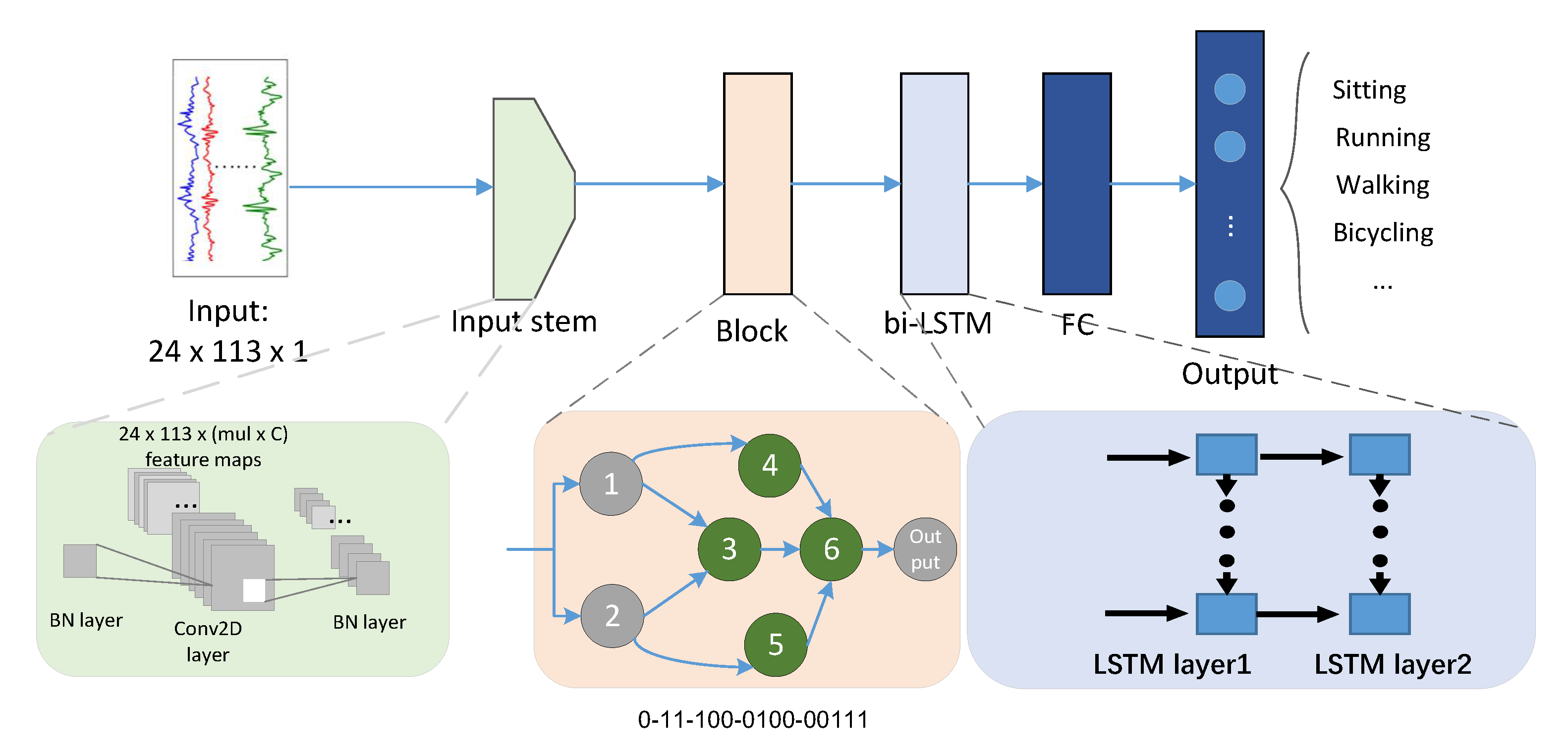
3. Approach
3.1. The Overall Operation of EAs
3.2. Architecture Encoding
3.3. Optimization Procedure
| Algorithm 1 HARNAS Search Algorithm for Neural Architectures |
| Input: Search space (e.g., hyperparameters including layers and blocks), fitness value (F), , Output: Best identifying network () of the Pareto optimal set.
|
3.3.1. Initial Population
3.3.2. Fitness Function
3.3.3. Mutation and Crossover
3.3.4. Non-Dominated Sorting
4. Experiment
4.1. Benchmark Datasets
4.2. Model Training
4.3. Analysis with Peer Competitors
5. Results
5.1. Multi-Model Classification
5.1.1. Convolutional Neural Network (CNN) with 1D-Convolution Kernels
5.1.2. LSTM
5.1.3. A Hybrid Model and DeepConvLSTM
5.1.4. DilatedSRU
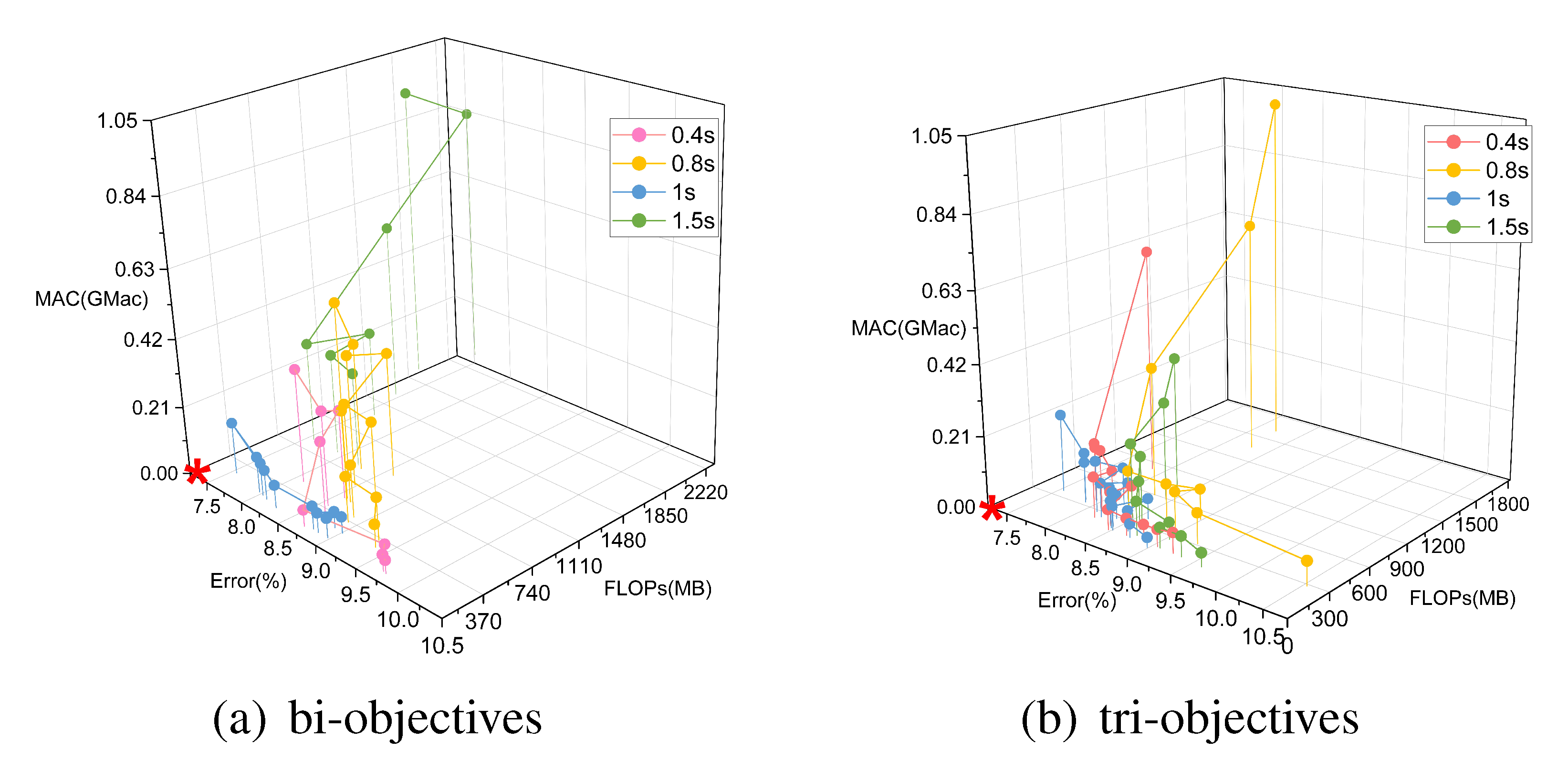
5.2. Multi-Objective Search
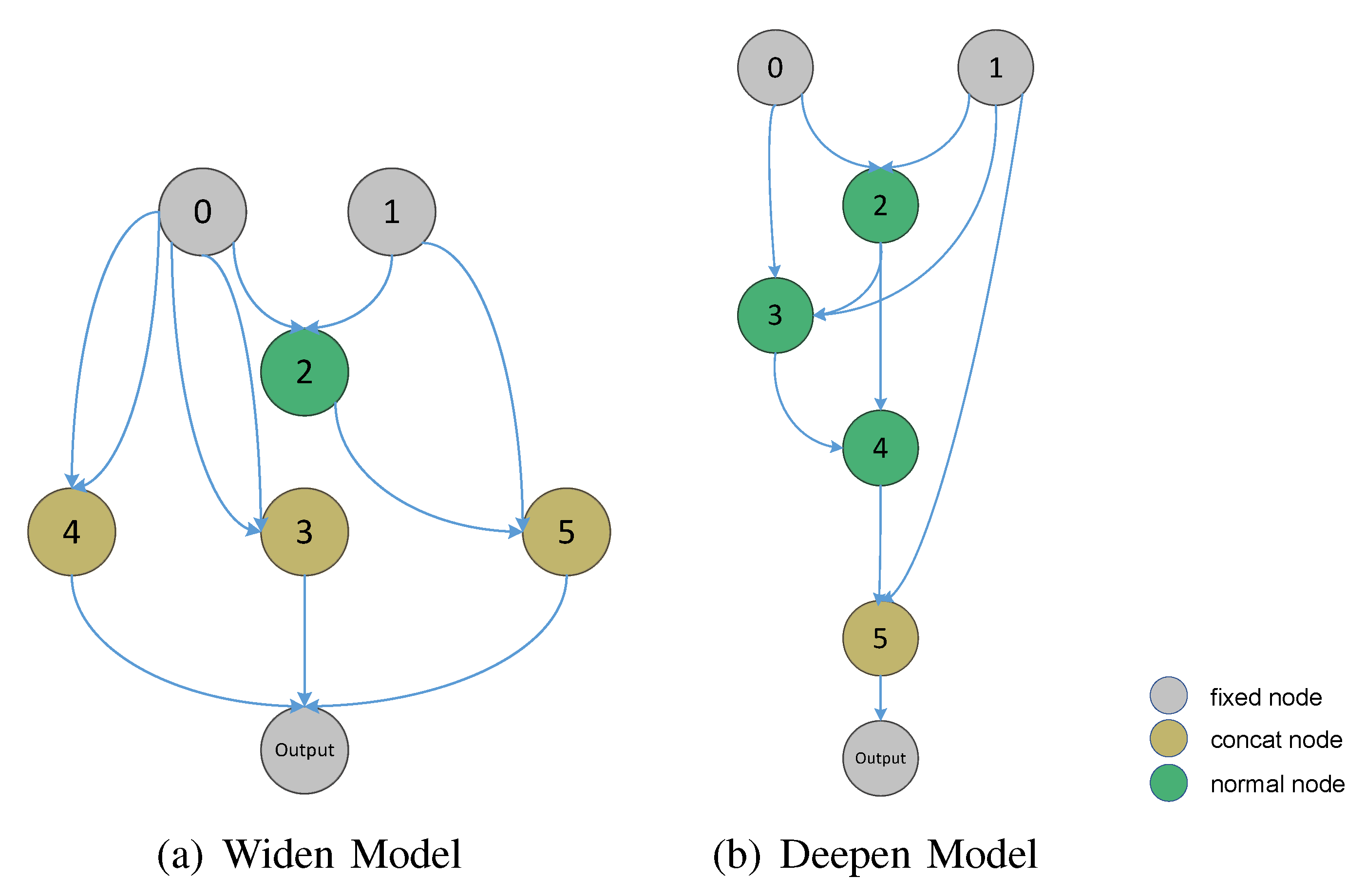
5.3. How Can Depth, Width, and Model Performance Be Quantitatively Evaluated?
5.4. Hyperparameter Evaluation
5.4.1. Length of the Sliding Window
5.4.2. Number of Nodes
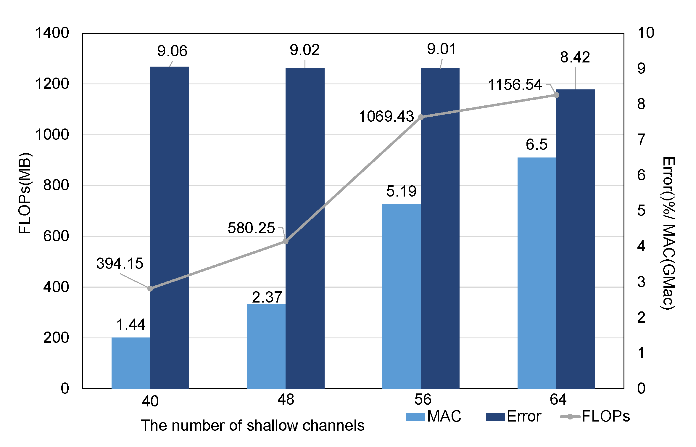
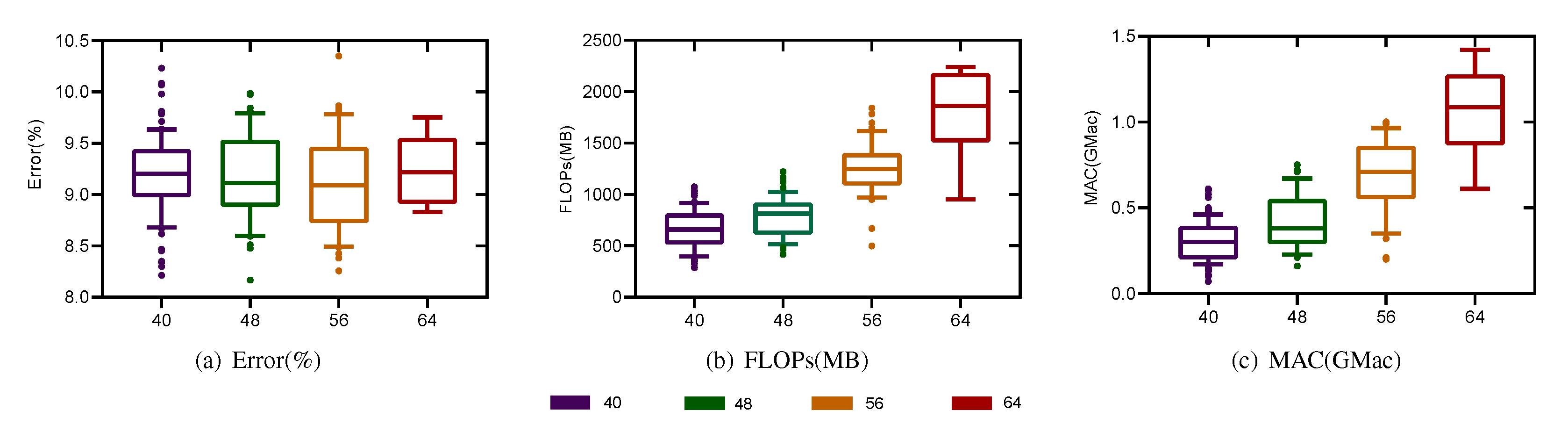
5.4.3. Number of Searched Channels
5.5. Data Representation Precision
6. Conclusions
Author Contributions
Funding
Institutional Review Board Statement
Informed Consent Statement
Data Availability Statement
Conflicts of Interest
References
- Xu, C.; He, J.; Zhang, X.; Yao, C.; Tseng, P.H. Geometrical kinematic modeling on human motion using method of multi-sensor fusion. Inf. Fusion 2018, 41, 243–254. [Google Scholar] [CrossRef]
- LeCun, Y.; Bengio, Y.; Hinton, G. Deep learning. Nature 2015, 521, 436–444. [Google Scholar] [CrossRef] [PubMed]
- Nweke, H.F.; Teh, Y.W.; Mujtaba, G.; Al-garadi, M.A. Data fusion and multiple classifier systems for human activity detection and health monitoring: Review and open research directions. Inf. Fusion 2019, 46, 147–170. [Google Scholar] [CrossRef]
- Xi, R.; Li, M.; Hou, M.; Fu, M.; Qu, H.; Liu, D.; Haruna, C.R. Deep dilation on multimodality time series for human activity recognition. IEEE Access 2018, 6, 53381–53396. [Google Scholar] [CrossRef]
- Francisco, O.; Daniel, R. Deep Convolutional and LSTM Recurrent Neural Networks for Multimodal Wearable Activity Recognition. Sensors 2016, 16, 115. [Google Scholar]
- Thornton, C.; Hutter, F.; Hoos, H.H.; Leyton-Brown, K. Auto-weka: Combined selection and hyperparameter optimization of classification algorithms. In Proceedings of the 19th ACM SIGKDD International Conferenceon Knowledge Discovery and Data Mining, Chicago, IL, USA, 11–14 August 2013; pp. 847–855. [Google Scholar]
- Wallach, H. Computational social science & computer science + social data. Commun. ACM 2018, 61, 42–44. [Google Scholar]
- Liu, H.; Simonyan, K.; Vinyals, O.; Fernando, C.; Kavukcuoglu, K. Hierarchical representations for efficient architecture search. In Proceedings of the International Conference on Learning Representations, Vancouver Convention Center, Vancouver, BC, Canada, 30 April–3 May 2018; pp. 13–25. [Google Scholar]
- Al-Obaidy, F.; Momtahen, S.; Hossain, M.F.; Mohammadi, F. Encrypted Traffic Classification Based ML for Identifying Different Social Media Applications. In Proceedings of the 2019 IEEE Canadian Conference of Electrical and Computer Engineering (CCECE), Edmonton, AB, Canada, 5–8 May 2019; pp. 1–5. [Google Scholar]
- Ma, N.; Zhang, X.; Zheng, H.; Sun, J. Shufflenet V2: Practical guidelines for efficient CNN architecture design. In Proceedings of the European Conference on Computer Vision (ECCV), Munich, Germany, 8–14 September 2018; pp. 116–131. [Google Scholar]
- Menhour, I.; Abidine, M.; Fergani, B. A new activity classification method K-SVM using Smartphone data. In Proceedings of the 2019 International Conference on Advanced Electrical Engineering (ICAEE), Algiers, Algeria, 19–21 November 2019; pp. 1–5. [Google Scholar]
- Hossain, T.; Goto, H.; Ahad, M.A.R.; Inoue, S. Mukherjee, Study on Sensor-based Activity Recognition Having Missing Data. In Proceedings of the 7th International Conference on Informatics, Electronics & Vision (ICIEV) and 2018 2nd International Conference on Imaging, Vision & Pattern Recognition (icIVPR), Saratha Devi, Germany, 25–29 June 2018; pp. 556–561. [Google Scholar]
- Mobark, M.; Chuprat, S.; Mantoro, T. Improving the accuracy of complex activities recognition using accelerometer-embedded mobile phone classifiers. In Proceedings of the Second International Conference on Informatics and Computing (ICIC), Jayapura, Indonesia, 1–3 November 2017; pp. 1–5. [Google Scholar]
- Acharjee, D.; Mukherjee, A.; Mandal, J.K.; Mukherjee, N. Activity recognition system using inbuilt sensors of smart mobile phone and minimizing feature vectors. Microsyst. Technol. 2016, 22, 2715–2722. [Google Scholar] [CrossRef]
- Ronao, C.A.; Cho, S.B. Deep convolutional neural networks for human activity recognition with smartphone sensors. In Proceedings of the International Conference on Neural Information Processing, Istanbul, Turkey, 9–12 November 2015; pp. 9–12. [Google Scholar]
- Murad, A.; Pyun, J.Y. Deep recurrent neural networks for human activity recognition. Sensors 2017, 17, 2556. [Google Scholar] [CrossRef] [PubMed] [Green Version]
- Pham, H.; Guan, M.Y.; Zoph, B.; Le, Q.V.; Dean, J. Efficient neural architecture search via parameter sharing. In Proceedings of the 35th International Conference on Machine Learning, Stockholm, Sweden, 10–15 July 2018. [Google Scholar]
- Bender, G.; Liu, H.; Chen, B.; Chu, G.; Cheng, S.; Kindermans, P.J.; Le, Q.V. Can Weight Sharing Outperform Random Architecture Search? An Investigation With TuNAS. In Proceedings of the 2020 IEEE/CVF Conference on Computer Vision and Pattern Recognition (CVPR), Seattle, WA, USA, 13–19 June 2020; pp. 14311–14320. [Google Scholar]
- Guo, M.; Zhong, Z.; Wu, W.; Lin, D.; Yan, J. IRLAS: Inverse Reinforcement Learning for Architecture Search. In Proceedings of the 2019 IEEE/CVF Conference on Computer Vision and Pattern Recognition (CVPR), Long Beach, CA, USA, 16–20 June 2019; pp. 9013–9021. [Google Scholar]
- Tan, M.; Chen, B.; Pang, R.; Vasudevan, V.; Sandler, M.; Howard, A.; Le, Q.V. MnasNet: Platform-Aware Neural Architecture Search for Mobile. In Proceedings of the 2019 IEEE/CVF Conference on Computer Vision and Pattern Recognition (CVPR), Long Beach, CA, USA, 16–20 June 2019; pp. 2815–2823. [Google Scholar]
- Phan, H.; Liu, Z.; Huynh, D.; Savvides, M.; Cheng, K.-T.; Shen, Z. Binarizing MobileNet via Evolution-Based Searching. In Proceedings of the 2020 IEEE/CVF Conference on Computer Vision and Pattern Recognition (CVPR), Seattle, WA, USA, 13–19 June 2020; pp. 13417–13426. [Google Scholar]
- Guo, Z.; Zhang, X.; Mu, H.; Heng, W.; Liu, Z.; Wei, Y.; Sun, J. Single path one-shot neural architecture search with uniform sampling. arXiv 2019, arXiv:1904.00420. [Google Scholar]
- Chu, X.; Zhou, T.; Zhang, B.; Li, J. Fair DARTS: Eliminating Unfair Advantages in Differentiable Architecture Search; Springer: Cham, Switzerland, 2020. [Google Scholar]
- Hu, Y.B.; Wu, X.; He, R. TF-NAS: Rethinking Three Search Freedoms of Latency-Constrained Differentiable Neural Architecture Search. In Proceedings of the European Conference on Computer Vision, Glasgow, UK, 23–28 August 2020. [Google Scholar]
- Luo, R.; Tian, F.; Qin, T.; Liu, T. Neural Architecture Optimization. In Proceedings of the Thirty-Second Conference on Neural Information Processing Systems, Vancouver, BC, Canada, 8–14 December 2019; pp. 1–12. [Google Scholar]
- Lu, Z.; Whalen, I.; Boddeti, V.; Yashesh, D. Kalyanmoy, NSGA-Net: Neural architecture search using multi-objective genetic algorithm. In Proceedings of the Genetic and Evolutionary Computation Conference, Prague, Czech Republic, 13–17 July 2019; pp. 419–427. [Google Scholar]
- Chen, Z.; Zhu, Q.; Soh, Y.C.; Le, Z. SM-NAS: Structural-to-Modular Neural Architecture Search for Object Detection. Proc. AAAI Conf. Artif. Intell. 2020, 34, 12661–12668. [Google Scholar]
- Chen, W.; Wang, Y.; Yang, S.; Liu, C.; Zhang, L. You Only Search Once: A Fast Automation Framework for Single-Stage DNN/Accelerator Co-design. In Proceedings of the 2020 Design, Automation & Test in Europe Conference & Exhibition (DATE), Grenoble, France, 9–13 March 2020; pp. 1283–1286. [Google Scholar]
- Bottou, L.; Chapelle, O.; DeCoste, D.; Weston, J. Scaling Learning Algorithms toward AI. In Large-Scale Kernel Machines; MIT Press: Cambridge, MA, USA, 2007; pp. 321–359. [Google Scholar]
- Christopher, O. Understanding LSTM Networks. 2015. Available online: http://colah.github.io/posts/2015-08-Understanding-LSTMs/ (accessed on 15 October 2018).
- Roggen, D.; Calatroni, A.; Rossi, M.; Holleczek, T.; Forster, K.; Troster, G.; Lukowicz, P.; Bannach, D.; Pirkl, G.; Ferscha, A.; et al. Collecting complex activity datasets in highly rich networked sensor environments. In Proceedings of the 2010 Seventh International Conference on Networked Sensing Systems (INSS), Kassel, Germany, 15–18 June 2010; pp. 233–240. [Google Scholar]
- Micucci, D.; Mobilio, M.; Napoletano, P. UniMiB SHAR: A new dataset for human activity recognition using acceleration data from smartphones. Appl. Sci. 2017, 7, 1101. [Google Scholar] [CrossRef] [Green Version]
- Li, F.; Shirahama, K.; Nisar, M.; Köping, L.; Grzegorzek, M. Comparison of feature learning methods for human activity recognition using wearable sensors. Sensors 2018, 18, 679. [Google Scholar] [CrossRef] [PubMed] [Green Version]
- Le Kernec, J.; Fioranelli, F.; Ding, C.; Zhao, H.; Sun, L.; Hong, H.; Lorandel, J.; Romain, O. Radar signal processing for sensing in assisted living: The challenges associated with real-time implementation of emerging algorithms. IEEE Signal Process. Mag. 2019, 36, 29–41. [Google Scholar] [CrossRef] [Green Version]


| Operation | Kernel Shape | Layers and Parameters | Values |
|---|---|---|---|
| Convolutional phase | N × 1 | 2D Conv. kernel size; 2D Conv. padding size | (11,1), (7,1), (5,1), (3,1), (1,1) (5,0), (3,0), (2,0), (1,0), (0,0) |
| N × N | 2D Conv. kernel size; 2D Conv. padding size | (7,7), (5,5), (3,3) (3,3), (2,2), (1,1) | |
| Dilated Convolutional phase | N × N | 2D Conv. kernel size; 2D Conv. padding size; 2D Conv. dilation rate; | (3,3), (5,5) (2,2), (4,4) (2,2) |
| Average Pooling Max Pooling phase | - | pooling kernel size; pooling padding size; | (3,1), (1,3), (3,3) (1,0), (0,1), (1,1) |
| skip connection | - | - | |
| Name | Equation | FLOPs |
|---|---|---|
| ReLU | 1 | |
| sigmoid | 4 | |
| tanh | 5 |
| Nodes = 2 | Nodes = 3 | ||||||
| Bi-objective | Concat | Error | FLOPs | MAC | Error | FLOPs | MAC |
| 1 | 9.203 | 453.822 | 0.215 | 9.080 | 504.070 | 0.273 | |
| 2 | 9.371 | 693.491 | 0.240 | 9.292 | 1012.617 | 0.490 | |
| 3 | - | - | - | 9.394 | 1243.817 | 0.440 | |
| 4 | - | - | - | - | - | - | |
| Tri-objective | 1 | 9.347 | 343.490 | 0.117 | 9.034 | 581.052 | 0.326 |
| 2 | 9.356 | 629.657 | 0.175 | 9.220 | 960.090 | 0.452 | |
| 3 | - | - | - | 9.425 | 1197.46 | 0.395 | |
| 4 | - | - | - | - | - | - | |
| Nodes = 4 | Nodes = 5 | ||||||
| Bi-objective | Concat | Error | FLOPs | MAC | Error | FLOPs | MAC |
| 1 | 9.007 | 640.422 | 0.340 | 9.158 | 564.878 | 0.344 | |
| 2 | 9.036 | 1023.15 | 0.540 | 9.000 | 883.453 | 0.440 | |
| 3 | 9.177 | 1324.275 | 0.511 | 9.223 | 1148.177 | 0.462 | |
| 4 | - | - | - | 9.750 | 1472.120 | 0.407 | |
| Tri-objective | 1 | 8.972 | 643.806 | 0.386 | 9.066 | 498.816 | 0.275 |
| 2 | 9.281 | 954.581 | 0.458 | 9.135 | 847.844 | 0.390 | |
| 3 | 9.365 | 1201.516 | 0.432 | 9.383 | 1041.329 | 0.365 | |
| 4 | 10.074 | 1710.425 | 0.615 | 9.611 | 1250.388 | 0.340 | |
| Operation Name | Parameters | ||
|---|---|---|---|
| Padding (P) | Stride (S) | Expansion Rate (D) | |
| Normal convolution | 1 | 1 | 1 |
| Dilated convolution | 1 | 1 | 2 |
| - | common hyperparameter: = 32 = 32 = 12 = 24 | ||
| Milliseconds/Iterations/Batch | Memory (MB) | F1 Score (%) | |
|---|---|---|---|
| FP32 | 36.58 | 30.66 | 92.16 |
| FP64 | 37.37 | 61.32 | 91.039 |
Publisher’s Note: MDPI stays neutral with regard to jurisdictional claims in published maps and institutional affiliations. |
© 2021 by the authors. Licensee MDPI, Basel, Switzerland. This article is an open access article distributed under the terms and conditions of the Creative Commons Attribution (CC BY) license (https://creativecommons.org/licenses/by/4.0/).
Share and Cite
Wang, X.; Wang, X.; Lv, T.; Jin, L.; He, M. HARNAS: Human Activity Recognition Based on Automatic Neural Architecture Search Using Evolutionary Algorithms. Sensors 2021, 21, 6927. https://doi.org/10.3390/s21206927
Wang X, Wang X, Lv T, Jin L, He M. HARNAS: Human Activity Recognition Based on Automatic Neural Architecture Search Using Evolutionary Algorithms. Sensors. 2021; 21(20):6927. https://doi.org/10.3390/s21206927
Chicago/Turabian StyleWang, Xiaojuan, Xinlei Wang, Tianqi Lv, Lei Jin, and Mingshu He. 2021. "HARNAS: Human Activity Recognition Based on Automatic Neural Architecture Search Using Evolutionary Algorithms" Sensors 21, no. 20: 6927. https://doi.org/10.3390/s21206927
APA StyleWang, X., Wang, X., Lv, T., Jin, L., & He, M. (2021). HARNAS: Human Activity Recognition Based on Automatic Neural Architecture Search Using Evolutionary Algorithms. Sensors, 21(20), 6927. https://doi.org/10.3390/s21206927