
Validation of 3-Space Wireless Inertial Measurement Units Using an Industrial Robot


Abstract
:1. Introduction
2. Materials and Methods
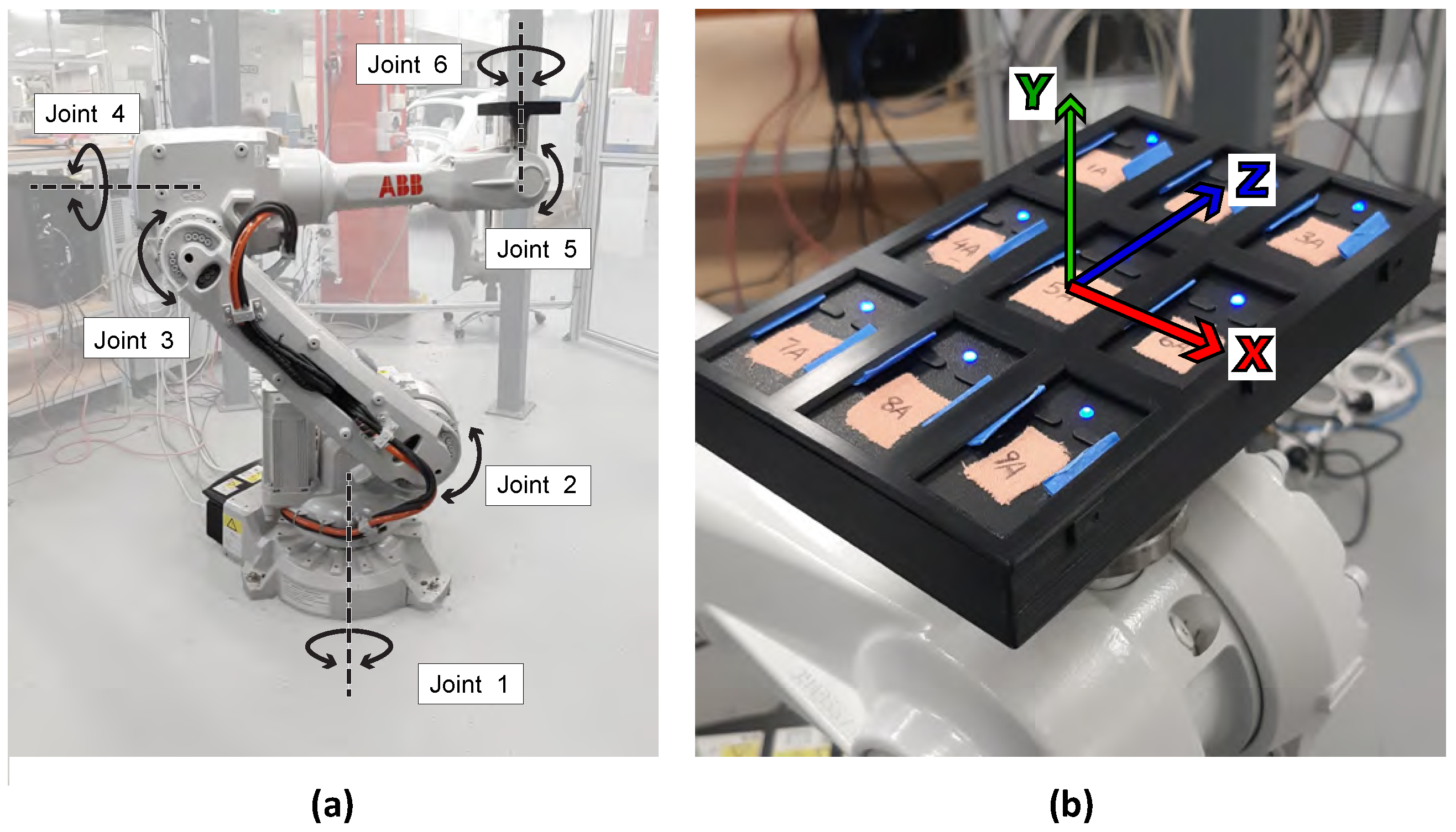
2.1. Measurement Setup
2.2. Measurement Protocol
2.3. Data Analysis
3. Results
4. Discussion
5. Conclusions
Author Contributions
Funding
Institutional Review Board Statement
Informed Consent Statement
Data Availability Statement
Acknowledgments
Conflicts of Interest
References
- Marin, J.; Blanco, T.; Marin, J.J. Octopus: A design methodology for motion capture wearables. Sensors 2017, 17, 1875. [Google Scholar] [CrossRef] [PubMed] [Green Version]
- Robert-Lachaine, X.; Mecheri, H.; Larue, C.; Plamondon, A. Validation of inertial measurement units with an optoelectronic system for whole-body motion analysis. Med. Biol. Eng. Comput. 2017, 55, 609–619. [Google Scholar] [CrossRef] [PubMed]
- Abyarjoo, F.; O-Larnnithipong, N.; Tangnimitchok, S.; Ortega, F.; Barreto, A. PostureMonitor: Real-time IMU wearable technology to foster poise and health. In Design, User Experience, and Usability: Interactive Experience Design; Marcus, A., Ed.; Springer International Publishing: Cham, Switzerland, 2015; pp. 543–552. [Google Scholar]
- Yan, X.; Li, H.; Li, A.R.; Zhang, H. Wearable IMU-based real-time motion warning system for construction workers’ musculoskeletal disorders prevention. Autom. Constr. 2017, 74, 2–11. [Google Scholar] [CrossRef]
- Williams, B.; Ryu, J.; Bourdon, P.; Graham-Smith, P.; Sinclair, P. Reliability and Validation of an Inertial Sensor Used to Measure Orientation Angle. In Proceedings of the 34th International Conference on Biomechanics in Sport, Tsukuba, Japan, 18–22 July 2016. [Google Scholar]
- Ligorio, G.; Zanotto, D.; Sabatini, A.; Agrawal, S. A novel functional calibration method for real-time elbow joint angles estimation with magnetic-inertial sensors. J. Biomech. 2017, 54, 106–110. [Google Scholar] [CrossRef] [PubMed]
- de Vries, W.; Veeger, H.; Baten, C.; van der Helm, F. Magnetic distortion in motion labs, implications for validating inertial magnetic sensors. Gait Posture 2009, 29, 535–541. [Google Scholar] [CrossRef] [PubMed]
- Madgwick, S.O.H.; Harrison, A.J.L.; Vaidyanathan, R. Estimation of IMU and MARG orientation using a gradient descent algorithm. In Proceedings of the 2011 IEEE International Conference on Rehabilitation Robotics, Zurich, Switzerland, 29 June–1 July 2011; pp. 1–7. [Google Scholar]
- Islam, T.; Islam, M.S.; Shajid-Ul-Mahmud, M.; Hossam-E-Haider, M.; Hossain, A. Comparison of complementary and Kalman filter based data fusion for attitude heading reference system. AIP Conf. Proc. 2017, 1919, 020002. [Google Scholar] [CrossRef] [Green Version]
- Maybeck, P.S. The Kalman filter: An introduction to concepts. In Autonomous Robot Vehicles; Springer: New York, NY, USA, 1990; pp. 194–204. [Google Scholar]
- Boonstra, M.C.; van der Slikke, R.M.; Keijsers, N.L.; van Lummel, R.C.; de Waal Malefijt, M.C.; Verdonschot, N. The accuracy of measuring the kinematics of rising from a chair with accelerometers and gyroscopes. J. Biomech. 2006, 39, 354–358. [Google Scholar] [CrossRef] [PubMed]
- Szeto, G.P.Y.; Cheng, S.W.K.; Poon, J.T.C.; Ting, A.C.W.; Tsang, R.C.C.; Ho, P. Surgeons’ static posture and movement repetitions in open and laparoscopic surgery. J. Surg. Res. 2012, 172, e19–e31. [Google Scholar] [CrossRef] [PubMed]
- Sers, R.; Forrester, S.; Zecca, M.; Ward, S.; Moss, E. Objective assessment of surgeon kinematics during simulated laparoscopic surgery: A preliminary evaluation of the effect of high body mass index models. Int. J. Comput. Assist. Radiol. Surg. 2021. [Google Scholar] [CrossRef] [PubMed]
- Parent, R. Chapter 2—Technical Background. In Computer Animation, 3rd ed.; Parent, R., Ed.; Morgan Kaufmann: Boston, MA, USA, 2012; pp. 33–60. [Google Scholar] [CrossRef]
- Yost Labs. 3-Space Sensor User’s Manual; Technical Report; Yost Labs: Portsmouth, OH, USA, 2017. [Google Scholar]
- Zhang, J.T.; Novak, A.C.; Brouwer, B.; Li, Q. Concurrent validation of Xsens MVN measurement of lower limb joint angular kinematics. Physiol. Meas. 2013, 34, N63–N69. [Google Scholar] [CrossRef] [PubMed]
- Robert-Lachaine, X.; Mecheri, H.; Muller, A.; Larue, C.; Plamondon, A. Validation of a low-cost inertial motion capture system for whole-body motion analysis. J. Biomech. 2020, 99, 109520. [Google Scholar] [CrossRef] [PubMed]
- Mihcin, S.; Kose, H.; Cizmeciogullari, S.; Ciklacandir, S.; Kocak, M.; Tosun, A.; Akan, A. Investigation of wearable motion capture system towards biomechanical modelling. In Proceedings of the 2019 IEEE International Symposium on Medical Measurements and Applications (MeMeA), Istanbul, Turkey, 26–28 June 2019; pp. 1–5. [Google Scholar] [CrossRef]
- Zügner, R.; Tranberg, R.; Timperley, J.; Hodgins, D.; Mohaddes, M.; Kärrholm, J. Validation of inertial measurement units with optical tracking system in patients operated with total hip arthroplasty. BMC Musculoskelet. Disord. 2019, 20, 52. [Google Scholar] [CrossRef] [PubMed] [Green Version]
- Ferrari, A.; Cutti, A.G.; Garofalo, P.; Raggi, M.; Heijboer, M.; Cappello, A.; Davalli, A. First in vivo assessment of “Outwalk”: A novel protocol for clinical gait analysis based on inertial and magnetic sensors. Med. Biol. Eng. Comput. 2009, 48, 1. [Google Scholar] [CrossRef] [PubMed]


| Filter | Static Trust Value | Confidence Range | |
|---|---|---|---|
| Minimum | Maximum | ||
| QComp | — | 0.00001 | 0.010 |
| QGrad | 0.057 | — | — |
| Kalman | — | 0.001 | 0.063 |
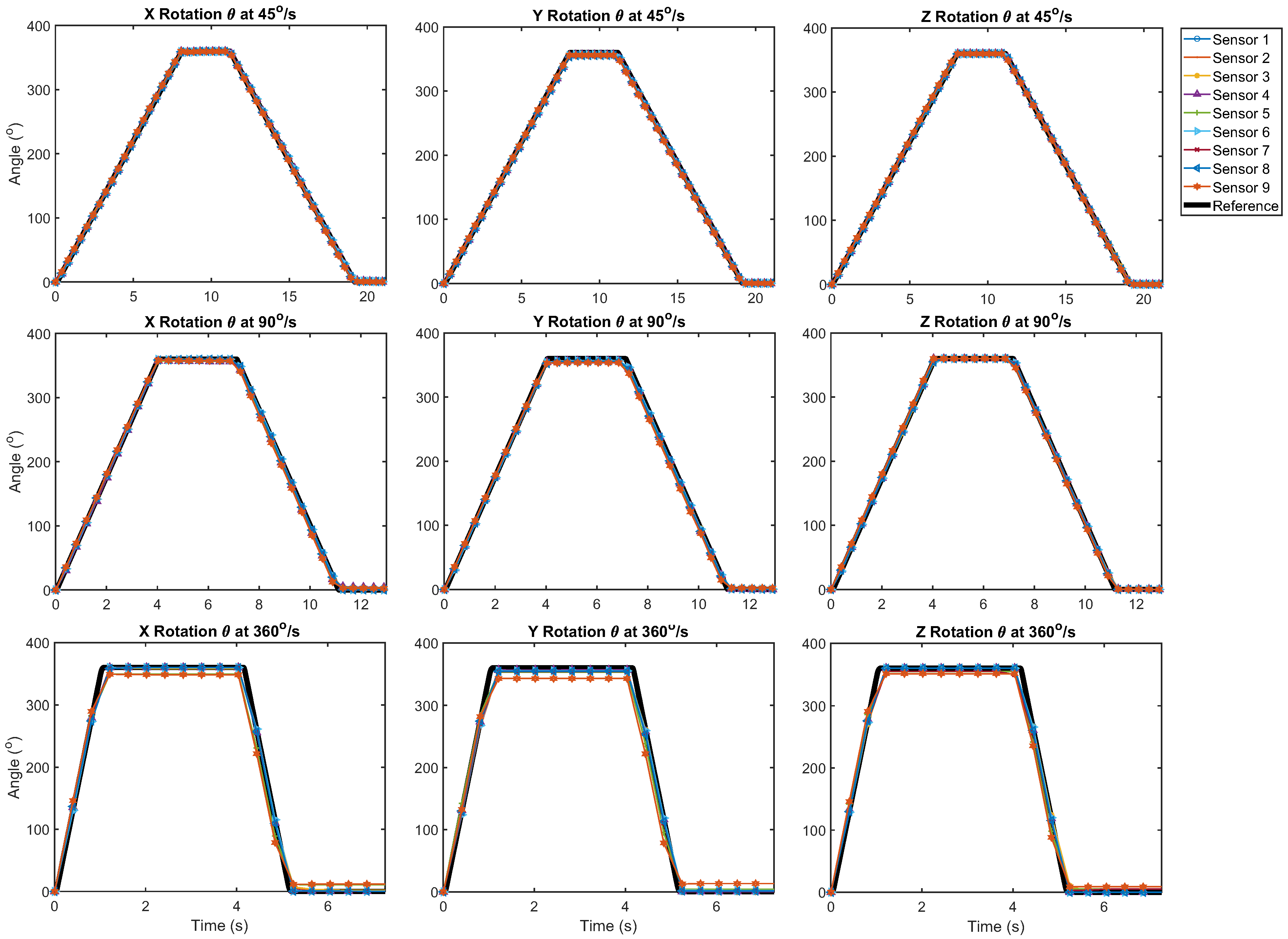
| Motion Sequence | Axis in Local Sensor Coordinate System | Axis in Work-Object Coordinate System | Starting Position | Motion |
|---|---|---|---|---|
| Rotation | X | X | J1: 45°, J2: —45°, J3: 45°, | J4: 0°→ —360°, —360°→ 0° |
| J4: 0°, J5: —90°, J6: —90° | ||||
| Y | Z | J1: 45°, J2: —45°, J3: 45°, | J6: —90°→ 270°, 270°→ —90° | |
| J4: 0°, J5: —90°, J6: —90° | ||||
| Z | Y | J1: 45°, J2: —45°, J3: 45°, | J4: 0°→ —360°, —360°→ 0° | |
| J4: 0°, J5: —90°, J6: 0° | ||||
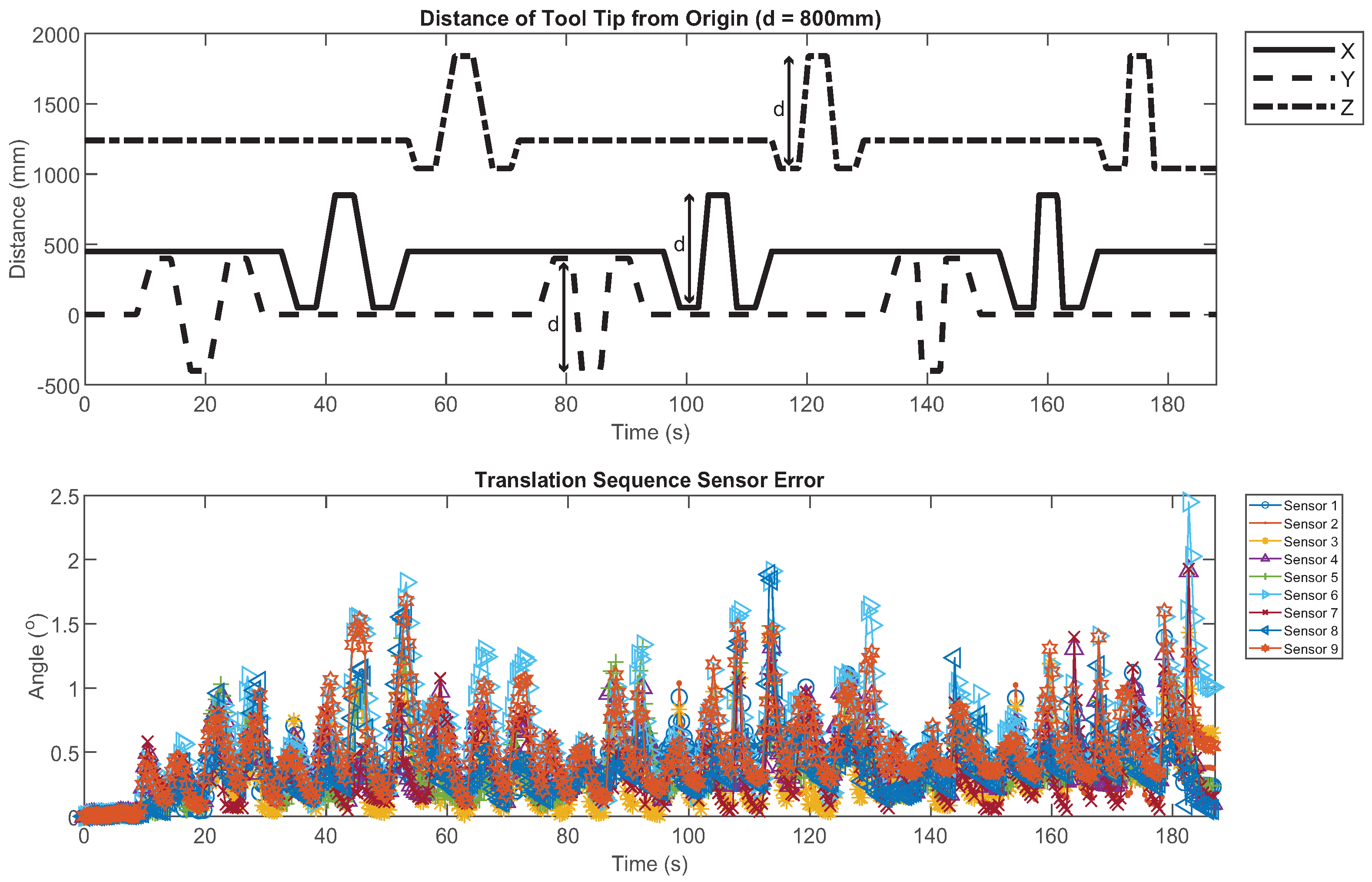
| Translation | X | X | J1: 45°, J2: —45°, J3: 45°, | TCP: (450, 0, 1240) → (50, 0, 1240), |
| J4: 0°, J5: —90°, J6: —90° | (50, 0, 1240) → (850, 0, 1240), | |||
| (850, 0, 1240) → (50, 0, 1240), | ||||
| (50, 0, 1240) → (450, 0, 1240) | ||||
| Y | Z | J1: 45°, J2: —45°, J3: 45°, | TCP: (450, 0, 1240) → (450, 0, 1040), | |
| J4: 0°, J5: —90°, J6: —90° | (450, 0, 1040) → (450, 0, 1840), | |||
| (450, 0, 1840) → (450, 0, 1040), | ||||
| (450, 0, 1040) → (450, 0, 1240) | ||||
| Z | Y | J1: 45°, J2: —45°, J3: 45°, | TCP: (450, 0, 1240) → (450, 400, 1240), | |
| J4: 0°, J5: —90°, J6: —90° | (450, 400, 1240) → (450, —400, 1240), | |||
| (450, —400, 1240) → (450, 400, 1240), | ||||
| (450, 400, 1240) → (450, 0, 1240) | ||||
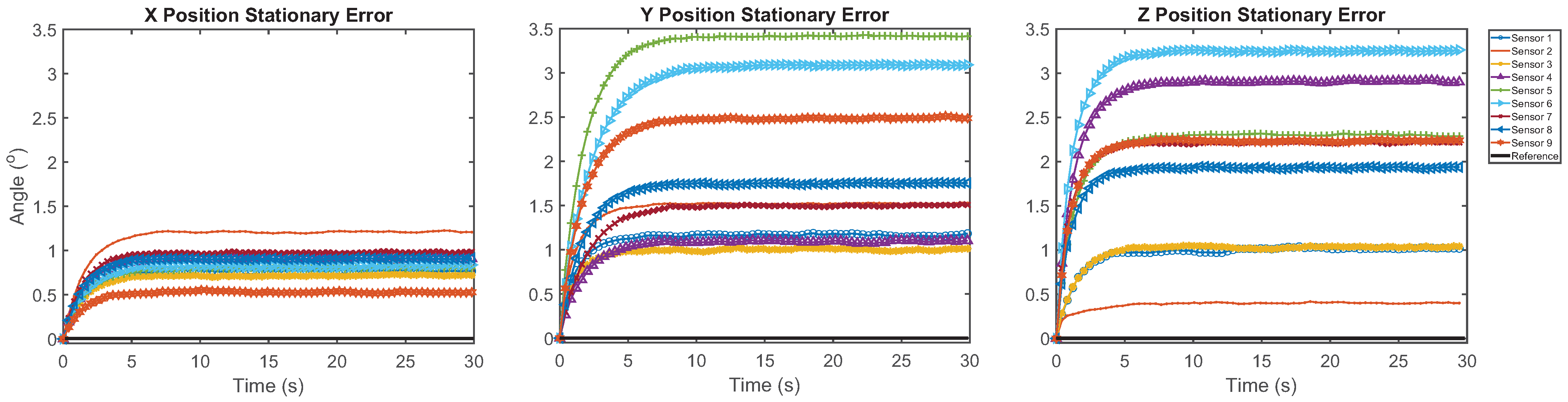
| Stationary | X | X | J1: 45°, J2: —45°, J3: 45°, | — |
| (30-s test) | J4: —90°, J5: —90°, J6: 180° | |||
| Y | Z | J1: 45°, J2: —45°, J3: 45°, | — | |
| J4: 0°, J5: —90°, J6: 0° | ||||
| Z | Y | J1: 45°, J2: —45°, J3: 45°, | — | |
| J4: —90°, J5: —90°, J6: 90° | ||||
| Stationary | Y | Z | J1: 45°, J2: —45°, J3: 45°, | — |
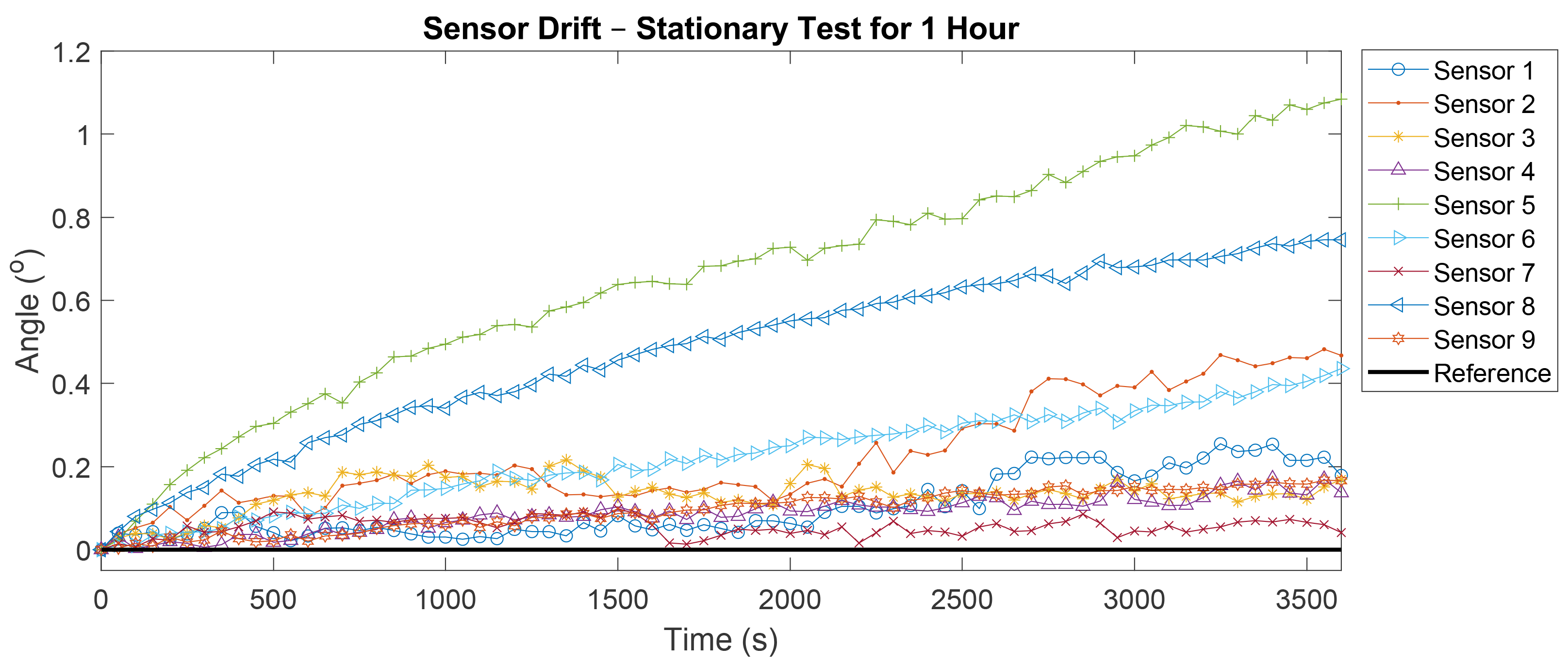
| (1-h test) | J4: 0°, J5: —90°, J6: 0° |
| Axis | Speed | QGrad without mag. | QComp without mag. | Kalman without mag. | Kalman with mag. |
|---|---|---|---|---|---|
| RMSE (°) | RMSE (°) | RMSE (°) | RMSE (°) | ||
| Rotation sequence | |||||
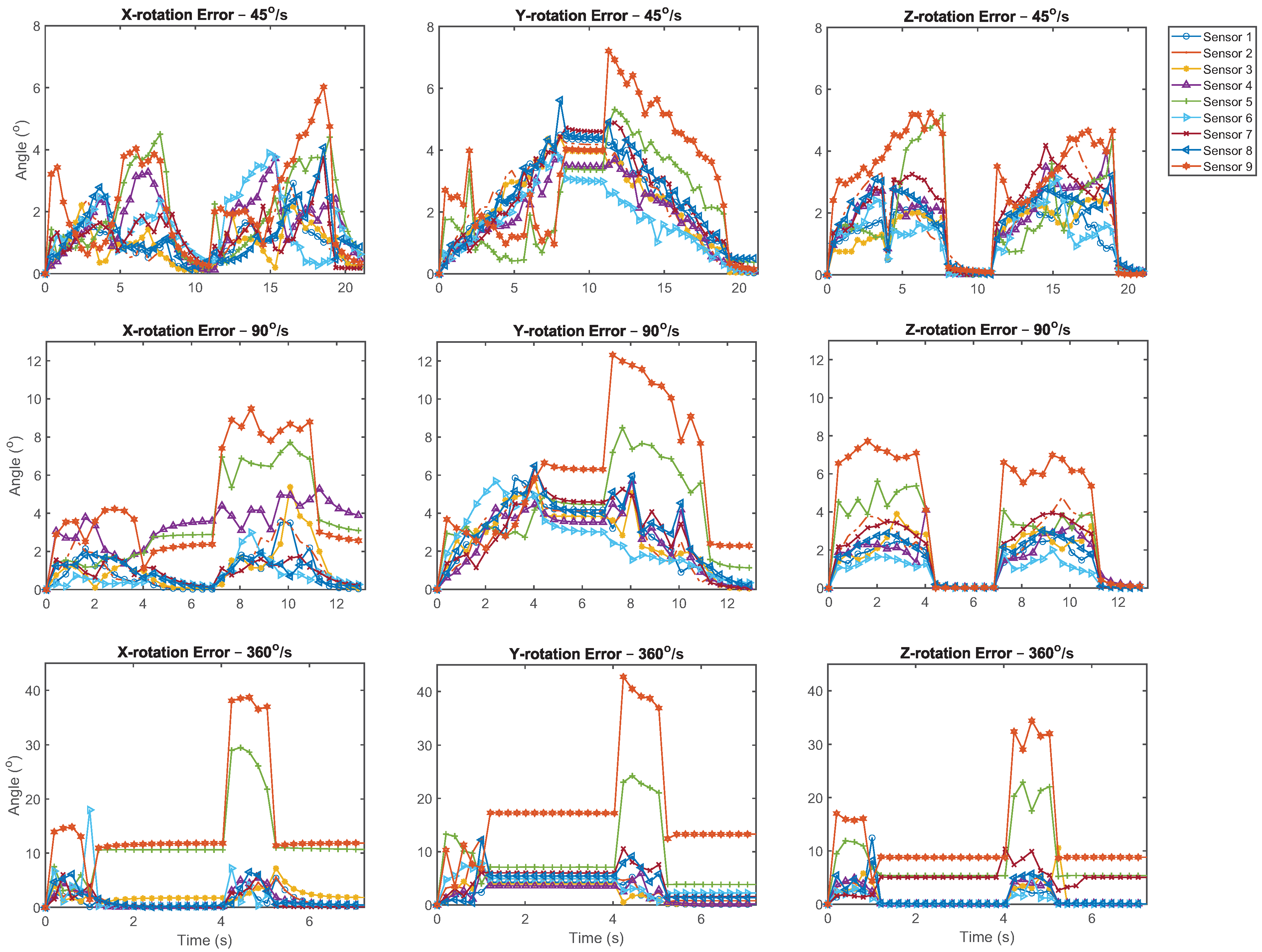
| X | 45°/s | 2.46 ± 1.62 | 2.76 ± 0.48 | 1.69 ± 0.56 | 44.13 ± 23.27 |
| 90°/s | 4.01 ± 3.51 | 3.94 ± 1.50 | 2.30 ± 1.63 | 26.97 ± 17.54 | |
| 360°/s | 10.70 ± 11.02 | 9.51 ± 5.10 | 5.20 ± 5.92 | 9.83 ± 6.44 | |
| Y | 45°/s | 4.55 ± 1.45 | 3.99 ± 0.92 | 2.80 ± 0.47 | 47.28 ± 32.48 |
| 90°/s | 5.14 ± 3.16 | 6.02 ± 1.63 | 3.75 ± 1.31 | 31.71 ± 29.89 | |
| 360°/s | 10.41 ± 7.62 | 9.11 ± 4.25 | 6.55 ± 5.55 | 7.05 ± 4.58 | |
| Z | 45°/s | 2.75 ± 1.49 | 2.64 ± 0.45 | 2.13 ± 0.57 | 38.81 ± 23.27 |
| 90°/s | 4.90 ± 4.16 | 3.68 ± 1.20 | 2.35 ± 1.18 | 28.10 ± 18.98 | |
| 360°/s | 12.5 ± 12.23 | 9.52 ± 4.89 | 4.92 ± 4.68 | 10.68 ± 7.02 | |
| Translation sequence | — | 0.24 ± 0.04 | 0.83 ± 0.05 | 0.48 ± 0.10 | 7.11 ± 4.10 |
| Stationary (30-s test) | |||||
| X | — | 2.67 ± 1.96 | 1.27 ± 0.58 | 0.82 ± 0.18 | 34.51 ± 28.65 |
| Y | — | 2.73 ± 2.83 | 1.33 ± 0.59 | 1.81 ± 0.84 | 2.88 ± 3.50 |
| Z | — | 1.78 ± 0.98 | 3.78 ± 1.87 | 1.86 ± 0.91 | 100 ± 57.84 |
| Axis | Speed | ANOVA p-Value (without mag.) | Multiple Comparison Test p-Value | ANOVA p-Value (with mag.) | ||
|---|---|---|---|---|---|---|
| QGrad v QComp | QGrad v Kalman | QComp v Kalman | ||||
| Rotation sequence | ||||||
| X | 45°/s | 0.0928 | — | — | — | <0.0001 * |
| 90°/s | 0.2483 | — | — | — | <0.0001 * | |
| 360°/s | 0.308 | — | — | — | 0.4187 | |
| Y | 45°/s | 0.0044 * | 0.4906 | 0.0037 * | 0.0532 | <0.0001 * |
| 90°/s | 0.1064 | — | — | — | <0.0001 * | |
| 360°/s | 0.3918 | — | — | — | 0.4456 | |
| Z | 45°/s | 0.3498 | — | — | — | <0.0001 * |
| 90°/s | 0.1359 | — | — | — | <0.0001 * | |
| 360°/s | 0.1535 | — | — | — | 0.2219 | |
| Translation sequence | — | <0.0001 * | <0.0001 * | <0.0001 * | <0.0001 * | <0.0001 * |
| Stationary (30-s test) | ||||||
| X | — | 0.008 * | 0.0499 * | 0.008 * | 0.7005 | <0.0001 * |
| Y | — | 0.2422 | — | — | — | 0.4365 |
| Z | — | 0.0052 * | 0.0101 * | 0.9908 | 0.0137 * | <0.0001 * |
| Filter | Speed | ANOVA p-Value | Multiple Comparison Test p-Value | ||
|---|---|---|---|---|---|
| X v Y | X v Z | Y v Z | |||
| QGrad | 45°/s | 0.0156 * | 0.0201 * | 0.9138 | 0.049 * |
| QComp | 45°/s | 0.0003 * | 0.0015 * | 0.9115 | 0.0005 * |
| Kalman | 45°/s | 0.007 * | 0.0005 * | 0.2082 | 0.0347 * |
| Filter | Speed | ANOVA p-Value | Multiple Comparison Test p-Value | ||
|---|---|---|---|---|---|
| 45°/s v 90°/s | 45°/s v 360°/s | 90°/s v 360°/s | |||
| Qgrad | X | 0.0372 * | 0.8775 | 0.0411 * | 0.1107 |
| Y | 0.0317 * | 0.9636 | 0.0429 * | 0.0736 | |
| Z | 0.027 * | 0.8182 | 0.0282 * | 0.0998 | |
| Qcomp | X | 0.0002 * | 0.6999 | 0.0003 * | 0.0022 |
| Y | 0.0018 * | 0.2625 | 0.0013 * | 0.0555 | |
| Z | <0.0001 * | 0.734 | 0.0001 * | 0.0008 * | |
| Kalman nomag | X | 0.1026 | — | — | — |
| Y | 0.0614 | — | — | — | |
| Z | 0.0834 | — | — | — | |
| Kalman mag | X | 0.0013 * | 0.1083 | 0.0008 * | 0.1088 |
| Y | 0.0098 * | 0.4149 | 0.0076 * | 0.124 | |
| Z | 0.0093 * | 0.4219 | 0.0072 * | 0.1165 | |
Publisher’s Note: MDPI stays neutral with regard to jurisdictional claims in published maps and institutional affiliations. |
© 2021 by the authors. Licensee MDPI, Basel, Switzerland. This article is an open access article distributed under the terms and conditions of the Creative Commons Attribution (CC BY) license (https://creativecommons.org/licenses/by/4.0/).
Share and Cite
Hislop, J.; Isaksson, M.; McCormick, J.; Hensman, C. Validation of 3-Space Wireless Inertial Measurement Units Using an Industrial Robot. Sensors 2021, 21, 6858. https://doi.org/10.3390/s21206858
Hislop J, Isaksson M, McCormick J, Hensman C. Validation of 3-Space Wireless Inertial Measurement Units Using an Industrial Robot. Sensors. 2021; 21(20):6858. https://doi.org/10.3390/s21206858
Chicago/Turabian StyleHislop, Jaime, Mats Isaksson, John McCormick, and Chris Hensman. 2021. "Validation of 3-Space Wireless Inertial Measurement Units Using an Industrial Robot" Sensors 21, no. 20: 6858. https://doi.org/10.3390/s21206858
APA StyleHislop, J., Isaksson, M., McCormick, J., & Hensman, C. (2021). Validation of 3-Space Wireless Inertial Measurement Units Using an Industrial Robot. Sensors, 21(20), 6858. https://doi.org/10.3390/s21206858