
Improving Machine Learning Classification Accuracy for Breathing Abnormalities by Enhancing Dataset

 , ,
, ,  ,
, 
 and
and 
Abstract
:1. Introduction
2. Literature Review
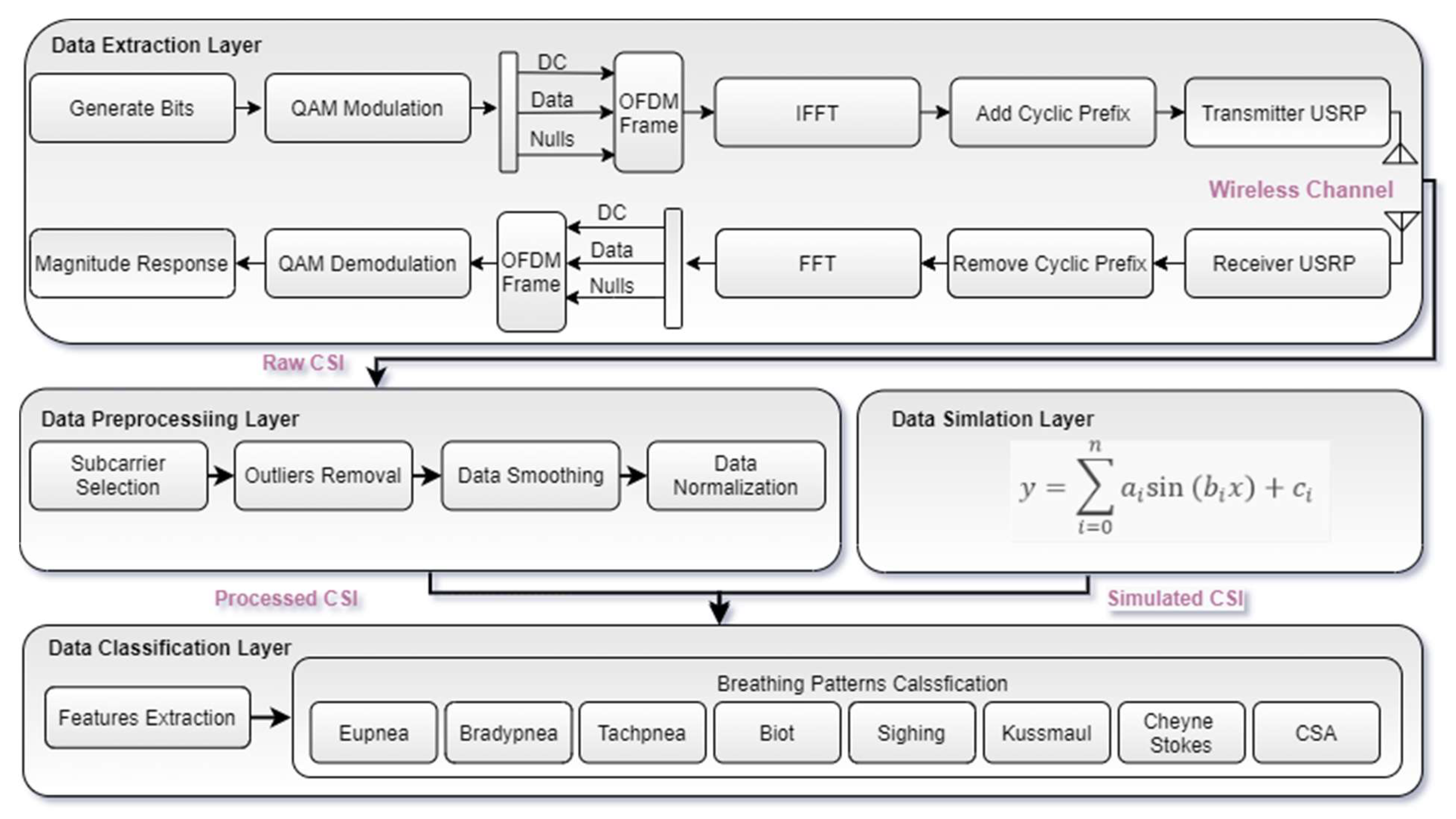
3. System Architecture
3.1. Data Extraction Layer
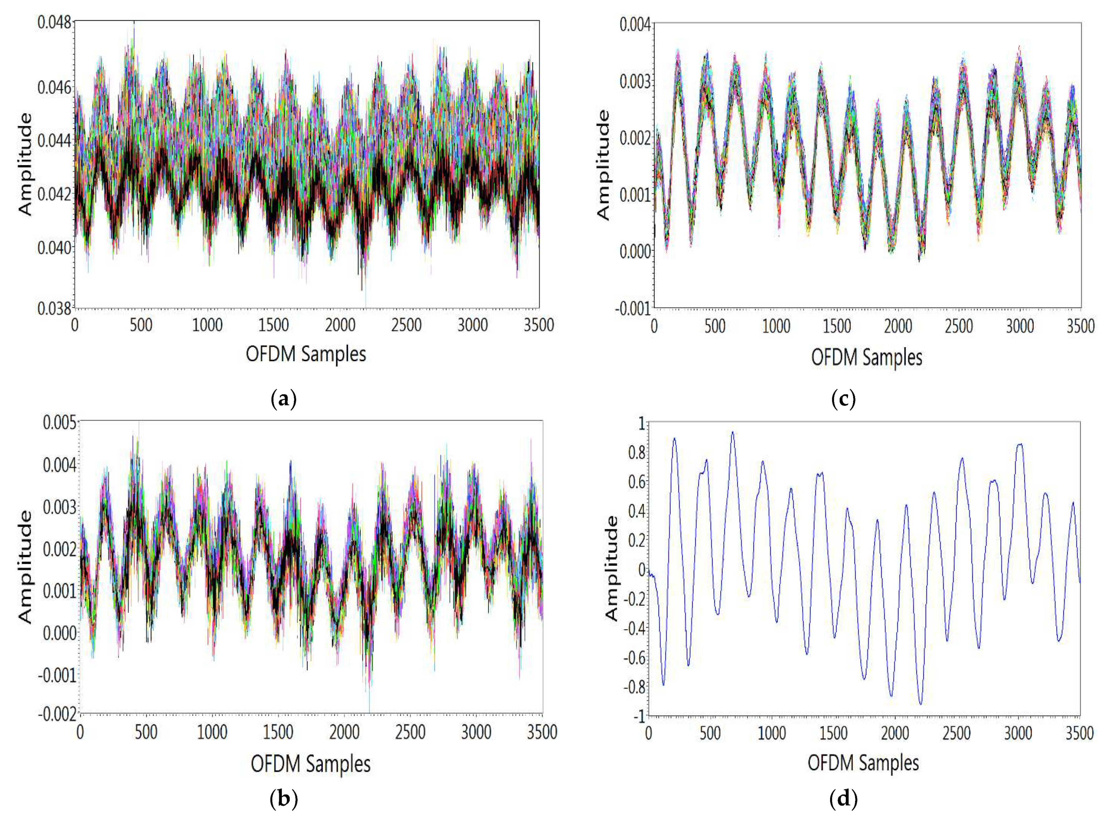
3.2. Data Preprocessing Layer
3.2.1. Subcarrier Selection
3.2.2. Outliers Removal
3.2.3. Data Smoothing
3.2.4. Data Normalization
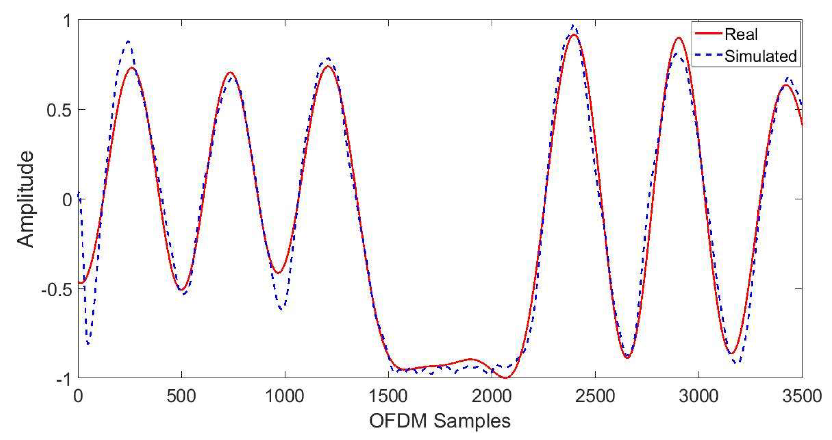
3.3. Data Simulation Layer
3.4. Data Classification Layer
4. Results and Discussion
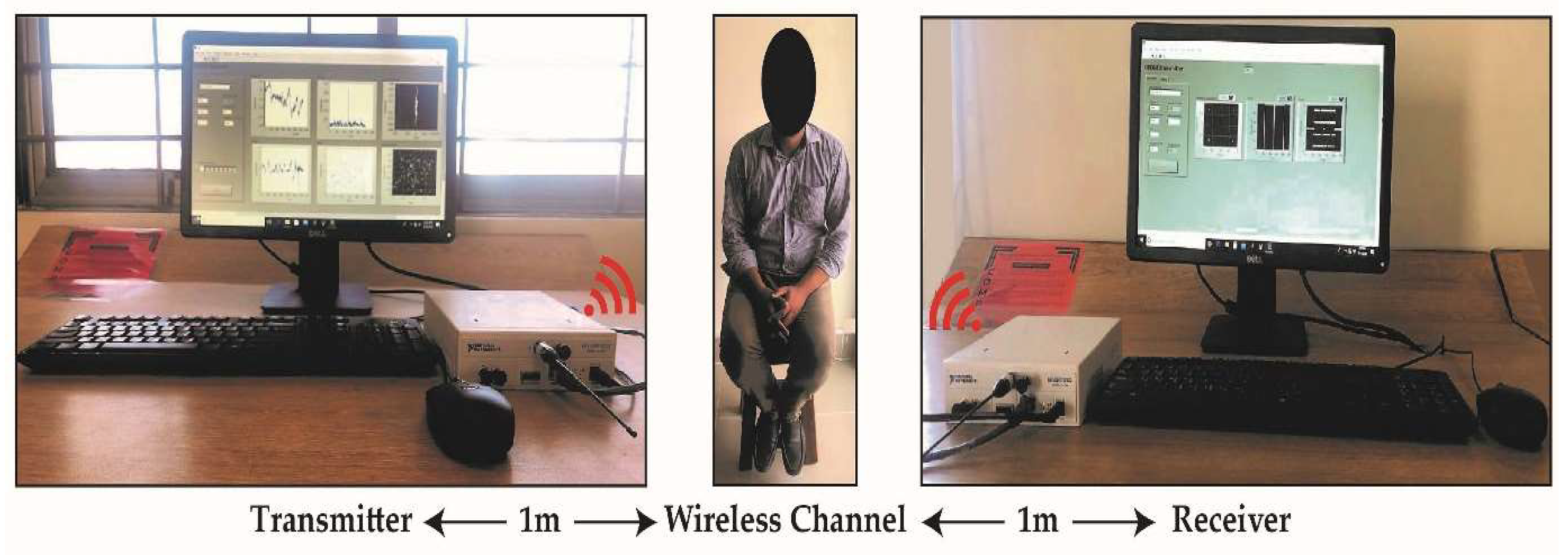
4.1. Experimental Setup
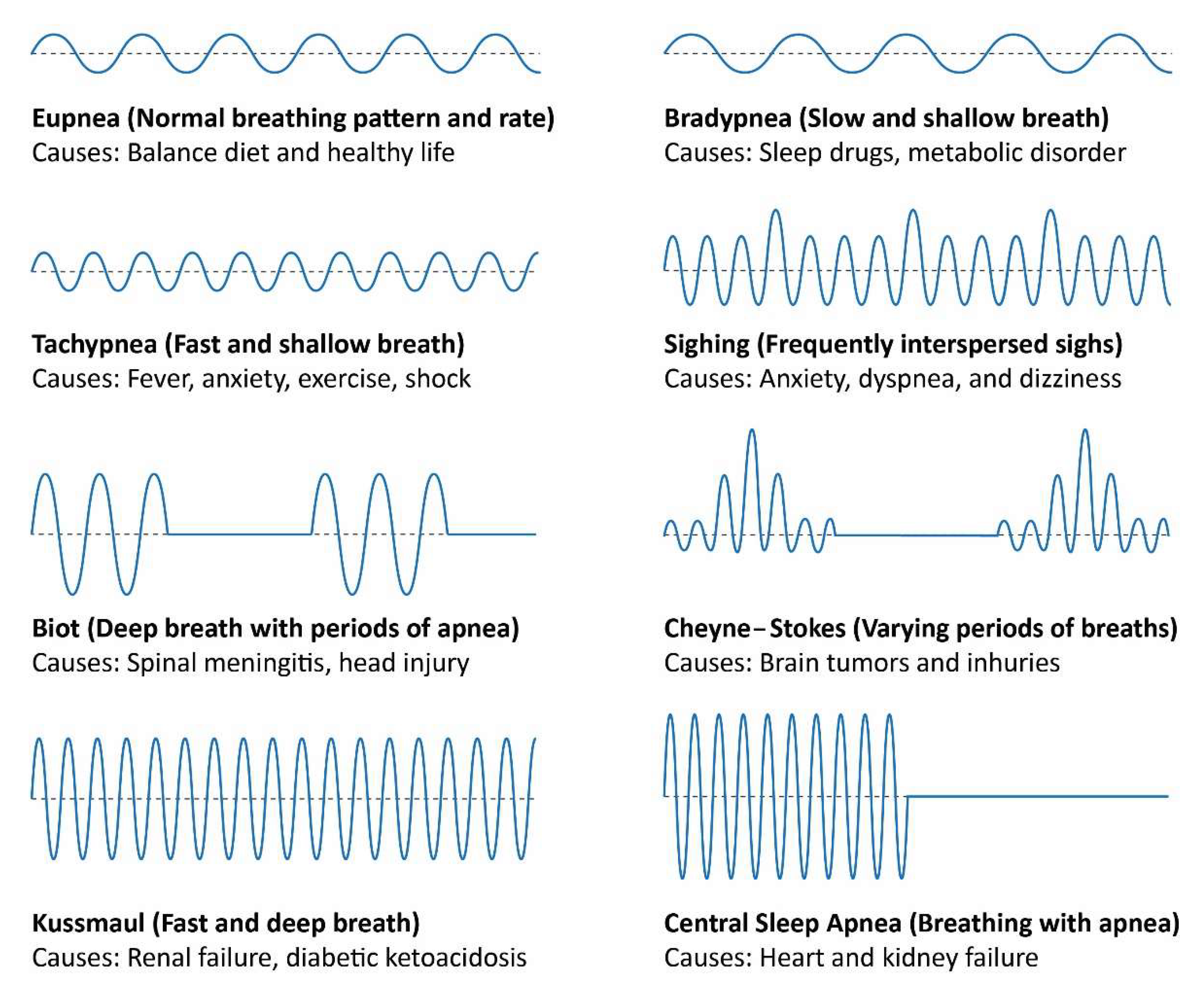
4.2. Breathing Patterns’ Monitoring
4.3. Breathing Patterns’ Classification
5. Conclusions
Author Contributions
Funding
Institutional Review Board Statement
Informed Consent Statement
Conflicts of Interest
References
- Zhou, F.; Yu, T.; Du, R.; Fan, G.; Liu, Y.; Liu, Z.; Xiang, J.; Wang, Y.; Song, B.; Gu, X. Clinical Course and Risk Factors for Mortality of Adult Inpatients with COVID-19 in Wuhan, China: A Retrospective Cohort Study. Lancet 2020, 395, 1054–1062. [Google Scholar] [CrossRef]
- Khan, M.B.; Zhang, Z.; Li, L.; Zhao, W.; Hababi, M.A.M.A.; Yang, X.; Abbasi, Q.H. A Systematic Review of Non-Contact Sensing for Developing a Platform to Contain COVID-19. Micromachines 2020, 11, 912. [Google Scholar] [CrossRef] [PubMed]
- Clinical Methods: The History, Physical, and Laboratory Examinations, 3rd ed.; Walker, H.K.; Hall, W.D.; Hurst, J.W. (Eds.) Butterworths: Boston, MA, USA, 1990; ISBN 978-0-409-90077-4. [Google Scholar]
- Xu, Z.; Shi, L.; Wang, Y.; Zhang, J.; Huang, L.; Zhang, C.; Liu, S.; Zhao, P.; Liu, H.; Zhu, L. Pathological Findings of COVID-19 Associated with Acute Respiratory Distress Syndrome. Lancet Resp. Med. 2020, 8, 420–422. [Google Scholar] [CrossRef]
- Von Schéele, B.H.C.; Von Schéele, I.A.M. The Measurement of Respiratory and Metabolic Parameters of Patients and Controls before and after Incremental Exercise on Bicycle: Supporting the Effort Syndrome Hypothesis. Appl. Psychophysiol. Biofeedback 1999, 24, 167–177. [Google Scholar] [CrossRef] [PubMed]
- Huang, C.; Wang, Y.; Li, X.; Ren, L.; Zhao, J.; Hu, Y.; Zhang, L.; Fan, G.; Xu, J.; Gu, X.; et al. Clinical features of patients infected with 2019 novel coronavirus in Wuhan, China. Lancet 2020, 395, 497–506. [Google Scholar] [CrossRef] [Green Version]
- Vafea, M.T.; Atalla, E.; Georgakas, J.; Shehadeh, F.; Mylona, E.K.; Kalligeros, M.; Mylonakis, E. Emerging Technologies for Use in the Study, Diagnosis, and Treatment of Patients with COVID-19. Cell. Mol. Bioeng. 2020, 13, 249–257. [Google Scholar] [CrossRef] [PubMed]
- Liaqat, D.; Abdalla, M.; Abed-Esfahani, P.; Gabel, M.; Son, T.; Wu, R.; Gershon, A.; Rudzicz, F.; Lara, E.D. WearBreathing: Real World Respiratory Rate Monitoring Using Smartwatches. Proc. ACM Int. Mobile Wearable Ubiquitous Technol. 2019, 3, 1–22. [Google Scholar] [CrossRef]
- Bae, M.; Lee, S.; Kim, N. Development of a Robust and Cost-Effective 3D Respiratory Motion Monitoring System Using the Kinect Device: Accuracy Comparison with the Conventional Stereovision Navigation System. Comput. Methods Prog. Biomed. 2018, 160, 25–32. [Google Scholar] [CrossRef] [PubMed]
- Shah, S.A.; Abbas, H.; Imran, M.A.; Abbasi, Q.H. RF Sensing for Healthcare Applications. In Backscattering and RF Sensing for Future Wireless Communication; John Wiley & Sons, Ltd.: London, UK, 2021; pp. 157–177. ISBN 978-1-119-69572-1. [Google Scholar]
- Chuma, E.L.; Iano, Y. A Movement Detection System Using Continuous-Wave Doppler Radar Sensor and Convolutional Neural Network to Detect Cough and Other Gestures. IEEE Sens. J. 2020, 21, 2921–2928. [Google Scholar] [CrossRef]
- Purnomo, A.T.; Lin, D.-B.; Adiprabowo, T.; Hendria, W.F. Non-Contact Monitoring and Classification of Breathing Pattern for the Supervision of People Infected by COVID-19. Sensors 2021, 21, 3172. [Google Scholar] [CrossRef] [PubMed]
- Adib, F.; Mao, H.; Kabelac, Z.; Katabi, D.; Miller, R.C. Smart Homes That Monitor Breathing and Heart Rate. In Proceedings of the 33rd Annual ACM Conference on Human Factors in Computing Systems, Seoul, Korea, 18–23 April 2015; Association for Computing Machinery: New York, NY, USA; pp. 837–846. [Google Scholar]
- Patwari, N.; Brewer, L.; Tate, Q.; Kaltiokallio, O.; Bocca, M. Breathfinding: A Wireless Network That Monitors and Locates Breathing in a Home. IEEE J. Select. Top. Sig. Proc. 2013, 8, 30–42. [Google Scholar] [CrossRef] [Green Version]
- Abdelnasser, H.; Harras, K.A.; Youssef, M. UbiBreathe: A Ubiquitous Non-Invasive WiFi-Based Breathing Estimator. In Proceedings of the 16th ACM International Symposium on Mobile Ad Hoc Networking and Computing, Hangzhou, China, 22–25 June 2015; Association for Computing Machinery: New York, NY, USA, 2015; pp. 277–286. [Google Scholar]
- Wang, Z.; Jiang, K.; Hou, Y.; Dou, W.; Zhang, C.; Huang, Z.; Guo, Y. A Survey on Human Behavior Recognition Using Channel State Information. IEEE Access 2019, 7, 155986–156024. [Google Scholar] [CrossRef]
- Schmidt, R. Multiple Emitter Location and Signal Parameter Estimation. IEEE Trans. Anten. Propag. 1986, 34, 276–280. [Google Scholar] [CrossRef] [Green Version]
- Wang, F.; Zhang, F.; Wu, C.; Wang, B.; Liu, K.R. Respiration Tracking for People Counting and Recognition. IEEE Int. Things J. 2020, 7, 5233–5245. [Google Scholar] [CrossRef]
- Shah, S.A.; Fioranelli, F. RF Sensing Technologies for Assisted Daily Living in Healthcare: A Comprehensive Review. IEEE Aerosp. Electron. Syst. Mag. 2019, 34, 26–44. [Google Scholar] [CrossRef] [Green Version]
- Al-Wahedi, A.; Al-Shams, M.; Albettar, M.A.; Alawsh, S.; Muqaibel, A. Wireless Monitoring of Respiration and Heart Rates Using Software-Defined-Radio. In Proceedings of the 2019 16th International Multi-Conference on Systems, Signals Devices (SSD), Istanbul, Turkey, 21–24 March 2019; pp. 529–532. [Google Scholar]
- Praktika, T.O.; Pramudita, A.A. Implementation of Multi-Frequency Continuous Wave Radar for Respiration Detection Using Software Defined Radio. In Proceedings of the 2020 10th Electrical Power, Electronics, Communications, Controls and Informatics Seminar (EECCIS), Malang, Indonesia, 26–28 August 2020; pp. 284–287. [Google Scholar]
- Rehman, M.; Shah, R.A.; Khan, M.B.; AbuAli, N.A.; Shah, S.A.; Yang, X.; Alomainy, A.; Imran, M.A.; Abbasi, Q.H. RF Sensing Based Breathing Patterns Detection Leveraging USRP Devices. Sensors 2021, 21, 3855. [Google Scholar] [CrossRef] [PubMed]
- Rehman, M.; Shah, R.A.; Khan, M.B.; Ali, N.A.A.; Alotaibi, A.A.; Althobaiti, T.; Ramzan, N.; Shaha, S.A.; Yang, X.; Alomainy, A. Contactless Small-Scale Movement Monitoring System Using Software Defined Radio for Early Diagnosis of COVID-19. IEEE Sens. J. 2021, 21, 17180–17188. [Google Scholar] [CrossRef]
- Muin, F.; Apriono, C. Path Loss and Human Body Absorption Experiment for Breath Detection. In Proceedings of the 2020 27th International Conference on Telecommunications (ICT), Bali, Indonesia, 5–7 October 2020; pp. 1–5. [Google Scholar]
- Lee, S.; Park, Y.-D.; Suh, Y.-J.; Jeon, S. Design and Implementation of Monitoring System for Breathing and Heart Rate Pattern Using WiFi Signals. In Proceedings of the 2018 15th IEEE Annual Consumer Communications Networking Conference (CCNC), Las Vegas, NV, USA, 12–15 January 2018; pp. 1–7. [Google Scholar]
- Khan, M.B.; Yang, X.; Ren, A.; Al-Hababi, M.A.M.; Zhao, N.; Guan, L.; Fan, D.; Shah, S.A. Design of Software Defined Radios Based Platform for Activity Recognition. IEEE Access 2019, 7, 31083–31088. [Google Scholar] [CrossRef]
- Van de Beek, J.-J.; Borjesson, P.O.; Boucheret, M.-L.; Landstrom, D.; Arenas, J.M.; Odling, P.; Ostberg, C.; Wahlqvist, M.; Wilson, S.K. A Time and Frequency Synchronization Scheme for Multiuser OFDM. IEEE J. Select. Areas Commun. 1999, 17, 1900–1914. [Google Scholar] [CrossRef] [Green Version]
- Wang, Y.; Hu, M.; Zhou, Y.; Li, Q.; Yao, N.; Zhai, G.; Zhang, X.-P.; Yang, X. Unobtrusive and Automatic Classification of Multiple People’s Abnormal Respiratory Patterns in Real Time Using Deep Neural Network and Depth Camera. IEEE Int. Things J. 2020, 7, 8559–8571. [Google Scholar] [CrossRef]
- Sum of Sines Models-MATLAB & Simulink. Available online: https://www.mathworks.com/help/curvefit/sum-of-sine.html (accessed on 18 August 2021).
- Add White Gaussian Noise to Signal-MATLAB Awgn. Available online: https://www.mathworks.com/help/comm/ref/awgn.html (accessed on 18 August 2021).


| Coefficients Values | Breathing Patterns | ||||||||
|---|---|---|---|---|---|---|---|---|---|
| Eupnea | Bradypnea | Tachypnea | Biot | Sighing | Kussmaul | Cheyne–Stokes | CSA | ||
| Amplitude | a1 | 0.506 | 0.409 | 0.406 | 0.435 | 0.256 | 0.547 | 0.775 | 0.427 |
| a2 | 0.342 | 0.303 | 0.326 | 0.260 | 0.333 | 0.282 | 0.302 | 0.437 | |
| a3 | 0.064 | 0.441 | 3.852 | 0.179 | 0.296 | 0.198 | 0.232 | 0.176 | |
| a4 | 0.077 | 0.174 | 1.838 | 0.564 | 0.192 | 0.192 | 6.850 | 0.329 | |
| a5 | 0.218 | 0.109 | 3.693 | 0.458 | 0.147 | 0.123 | 6.855 | 0.240 | |
| a6 | 0.043 | 0.075 | 0.066 | 0.237 | 0.179 | 0.120 | 0.205 | 0.202 | |
| a7 | 0.066 | 0.607 | 1.692 | 0.789 | 0.152 | 9.275 | 0.115 | 0.164 | |
| Frequency | b1 | 0.001 | 0.011 | 0.027 | 0.002 | 0.001 | 0.036 | 0.001 | 0.004 |
| b2 | 0.021 | 0.012 | 0.002 | 0.015 | 0.018 | 0.039 | 0.016 | 0.025 | |
| b3 | 0.005 | 0.001 | 0.025 | 0.010 | 0.011 | 0.003 | 0.004 | 0.000 | |
| b4 | 0.019 | 0.008 | 0.029 | 0.012 | 0.021 | 0.032 | 0.021 | 0.007 | |
| b5 | 0.003 | 0.014 | 0.025 | 0.004 | 0.004 | 0.025 | 0.021 | 0.018 | |
| b6 | 0.029 | 0.005 | 0.009 | 0.007 | 0.029 | 0.029 | 0.018 | 0.022 | |
| b7 | 0.022 | 0.001 | 0.029 | 0.001 | 0.007 | 0.000 | 0.005 | 0.011 | |
| Phase | c1 | 2.388 | −1.035 | −0.297 | 3.864 | −2.571 | −2.797 | 2.968 | 2.462 |
| c2 | −0.373 | 2.775 | 0.207 | −2.694 | −1.710 | −0.073 | 1.868 | 2.009 | |
| c3 | −1.513 | 3.456 | 2.941 | 3.302 | 2.123 | 0.331 | −2.013 | 0.944 | |
| c4 | 1.107 | −1.130 | 0.915 | −0.770 | 2.059 | −2.012 | −3.590 | −2.466 | |
| c5 | 2.434 | 1.926 | −0.119 | −2.595 | −1.478 | −1.583 | −0.497 | 2.735 | |
| c6 | −1.227 | 2.053 | −0.194 | −0.835 | −1.264 | −1.548 | 1.154 | −1.577 | |
| c7 | −0.075 | 1.091 | 4.008 | −4.899 | −1.650 | 3.133 | −1.390 | −1.952 | |
| Sr. No. | Statistical Features | Detail | Equations |
|---|---|---|---|
| 1 | Minimum | Minimum value in data | |
| 2 | Maximum | Maximum value in data | |
| 3 | Mean | Data mean | |
| 4 | Variance | Spread of data | |
| 5 | Standard deviation | Square root of variance | |
| 6 | Peak-to-peak value | Variations in data about the mean | |
| 7 | RMS | Root mean of square data | |
| 8 | Kurtosis | Peak sharpness of a frequency–distribution curve | |
| 9 | Skewness | Measure of symmetry in data | |
| 10 | Interquartile range | Mid-spread of data | |
| 11 | Waveform factor | Ratio of the RMS value to the mean value | |
| 12 | Peak factor | Ratio of maximum value of data to RMS | |
| 13 | FFT | Frequency information about data | |
| 14 | Frequency Min | Minimum frequency component | |
| 15 | Frequency Max | Maximum frequency component | |
| 16 | Spectral Probability | Probability distribution of spectrum | |
| 17 | Spectrum Entropy | Measure of data irregularity | |
| 18 | Signal Energy | Measure of energy component |
| Sr. No. | Gender | Age (Years) | Weight (Pounds) | Height (Inches) | Body Mass Index |
|---|---|---|---|---|---|
| 1 | Male | 26 | 168 | 68 | 25.4 |
| 2 | Male | 28 | 144 | 71 | 20.3 |
| 3 | Male | 31 | 114 | 70 | 16.8 |
| 4 | Male | 31 | 113 | 69 | 16.6 |
| 5 | Male | 31 | 143 | 68 | 21.5 |
| Algorithms | Actual/Predicted | Eupnea | Bradypnea | Tachypnea | Biot | Sighing | Kussmaul | Cheyne–Stokes | CSA |
|---|---|---|---|---|---|---|---|---|---|
| Cosine KNN | Eupnea | 3487 | 65 | 63 | 9 | 0 | 4 | 7 | 15 |
| Bradypnea | 58 | 3512 | 42 | 7 | 0 | 10 | 0 | 21 | |
| Tachypnea | 134 | 71 | 3396 | 24 | 0 | 1 | 13 | 11 | |
| Biot | 3 | 2 | 12 | 3620 | 3 | 4 | 6 | 0 | |
| Sighing | 0 | 0 | 0 | 0 | 3648 | 2 | 0 | 0 | |
| Kussmaul | 2 | 6 | 1 | 17 | 3 | 3618 | 3 | 0 | |
| Cheyne–Stokes | 0 | 0 | 0 | 8 | 0 | 4 | 3638 | 0 | |
| CSA | 43 | 29 | 31 | 1 | 0 | 0 | 0 | 3546 | |
| Complex Tree | Eupnea | 3491 | 74 | 0 | 76 | 0 | 0 | 9 | 0 |
| Bradypnea | 48 | 3596 | 0 | 4 | 0 | 0 | 2 | 0 | |
| Tachypnea | 0 | 0 | 3487 | 0 | 0 | 22 | 0 | 141 | |
| Biot | 54 | 3 | 0 | 3588 | 0 | 0 | 5 | 0 | |
| Sighing | 0 | 0 | 0 | 0 | 3649 | 1 | 0 | 0 | |
| Kussmaul | 0 | 0 | 55 | 0 | 2 | 3587 | 0 | 6 | |
| Cheyne–Stokes | 8 | 2 | 0 | 19 | 0 | 0 | 3621 | 0 | |
| CSA | 0 | 0 | 407 | 0 | 0 | 0 | 0 | 3243 | |
| Ensemble Boosted Tree | Eupnea | 2122 | 613 | 0 | 781 | 0 | 0 | 134 | 0 |
| Bradypnea | 101 | 3007 | 0 | 62 | 0 | 0 | 480 | 0 | |
| Tachypnea | 0 | 0 | 3372 | 0 | 0 | 162 | 0 | 116 | |
| Biot | 99 | 42 | 0 | 3478 | 0 | 0 | 31 | 0 | |
| Sighing | 0 | 0 | 0 | 0 | 3644 | 6 | 0 | 0 | |
| Kussmaul | 0 | 0 | 25 | 0 | 149 | 3461 | 0 | 15 | |
| Cheyne–Stokes | 6 | 0 | 0 | 282 | 0 | 0 | 3362 | 0 | |
| CSA | 0 | 0 | 1073 | 0 | 0 | 36 | 0 | 2541 | |
| Linear SVM | Eupnea | 2367 | 631 | 138 | 272 | 56 | 97 | 89 | |
| Bradypnea | 712 | 1958 | 174 | 476 | 118 | 93 | 43 | 76 | |
| Tachypnea | 2 | 0 | 2967 | 14 | 0 | 123 | 0 | 544 | |
| Biot | 519 | 497 | 32 | 2264 | 0 | 267 | 70 | 1 | |
| Sighing | 0 | 0 | 0 | 0 | 3449 | 201 | 0 | 0 | |
| Kussmaul | 0 | 0 | 50 | 191 | 71 | 3314 | 3 | 21 | |
| Cheyne–Stokes | 192 | 143 | 0 | 121 | 136 | 280 | 2778 | 0 | |
| CSA | 0 | 0 | 696 | 0 | 0 | 0 | 0 | 2954 |
| Algorithms | Actual /Predicted | Eupnea | Bradypnea | Tachypnea | Biot | Sighing | Kussmaul | Cheyne–Stokes | CSA |
|---|---|---|---|---|---|---|---|---|---|
| Cosine KNN | Eupnea | 13,493 | 43 | 77 | 3 | 0 | 7 | 4 | 23 |
| Bradypnea | 33 | 13,539 | 42 | 2 | 0 | 22 | 0 | 12 | |
| Tachypnea | 179 | 72 | 13,334 | 49 | 0 | 1 | 7 | 8 | |
| Biot | 4 | 3 | 36 | 13,604 | 0 | 3 | 0 | 0 | |
| Sighing | 0 | 0 | 0 | 0 | 13,648 | 0 | 2 | 0 | |
| Kussmaul | 3 | 5 | 0 | 1 | 1340 | 1 | 0 | ||
| Cheyne–Stokes | 2 | 0 | 0 | 3 | 1 | 1 | 13,642 | 1 | |
| CSA | 49 | 29 | 13 | 21 | 0 | 8 | 6 | 13,523 | |
| Complex Tree | Eupnea | 12,960 | 318 | 0 | 365 | 0 | 0 | 7 | 0 |
| Bradypnea | 68 | 13,491 | 0 | 84 | 0 | 0 | 2 | 5 | |
| Tachypnea | 1 | 0 | 13,352 | 0 | 0 | 94 | 0 | 203 | |
| Biot | 46 | 25 | 0 | 13,570 | 1 | 8 | |||
| Sighing | 0 | 0 | 0 | 0 | 13,629 | 21 | 0 | 0 | |
| Kussmaul | 0 | 0 | 14 | 0 | 1 | 13,621 | 0 | 3 | |
| Cheyne–Stokes | 113 | 12 | 0 | 45 | 0 | 0 | 13,480 | 0 | |
| CSA | 0 | 0 | 358 | 0 | 2 | 3 | 0 | 13,287 | |
| Ensemble Boosted Tree | Eupnea | 12,580 | 798 | 0 | 130 | 0 | 0 | 142 | 0 |
| Bradypnea | 375 | 12,955 | 0 | 0 | 0 | 0 | 320 | 0 | |
| Tachypnea | 0 | 0 | 13,252 | 0 | 0 | 325 | 0 | 73 | |
| Biot | 1003 | 496 | 0 | 12,134 | 0 | 0 | 18 | 0 | |
| Sighing | 0 | 0 | 0 | 0 | 13,499 | 151 | 0 | 0 | |
| Kussmaul | 0 | 0 | 1 | 0 | 152 | 13,456 | 0 | 41 | |
| Cheyne–Stokes | 127 | 61 | 0 | 6 | 0 | 0 | 13,456 | 0 | |
| CSA | 0 | 0 | 1377 | 0 | 120 | 59 | 0 | 12,094 | |
| Linear SVM | Eupnea | 10,003 | 0 | 0 | 0 | 3647 | 0 | 0 | 0 |
| Bradypnea | 1 | 9998 | 0 | 2 | 3649 | 0 | 0 | 0 | |
| Tachypnea | 17 | 0 | 10,027 | 0 | 3606 | 0 | 0 | 0 | |
| Biot | 0 | 0 | 3 | 10,000 | 3621 | 0 | 26 | 0 | |
| Sighing | 149 | 0 | 0 | 0 | 13,496 | 0 | 5 | 0 | |
| Kussmaul | 0 | 0 | 0 | 0 | 3650 | 10,284 | 0 | 0 | |
| Cheyne–Stokes | 0 | 0 | 0 | 0 | 3650 | 0 | 10,000 | 0 | |
| CSA | 0 | 0 | 0 | 0 | 3650 | 0 | 0 | 10,000 |
| Algorithms | Real-Time Breathing Data | Simulated Breathing Data | ||||
|---|---|---|---|---|---|---|
| Accuracy (%) | Prediction Speed (obs/s) | Training Time (s) | Accuracy (%) | Prediction Speed (obs/s) | Training Time (s) | |
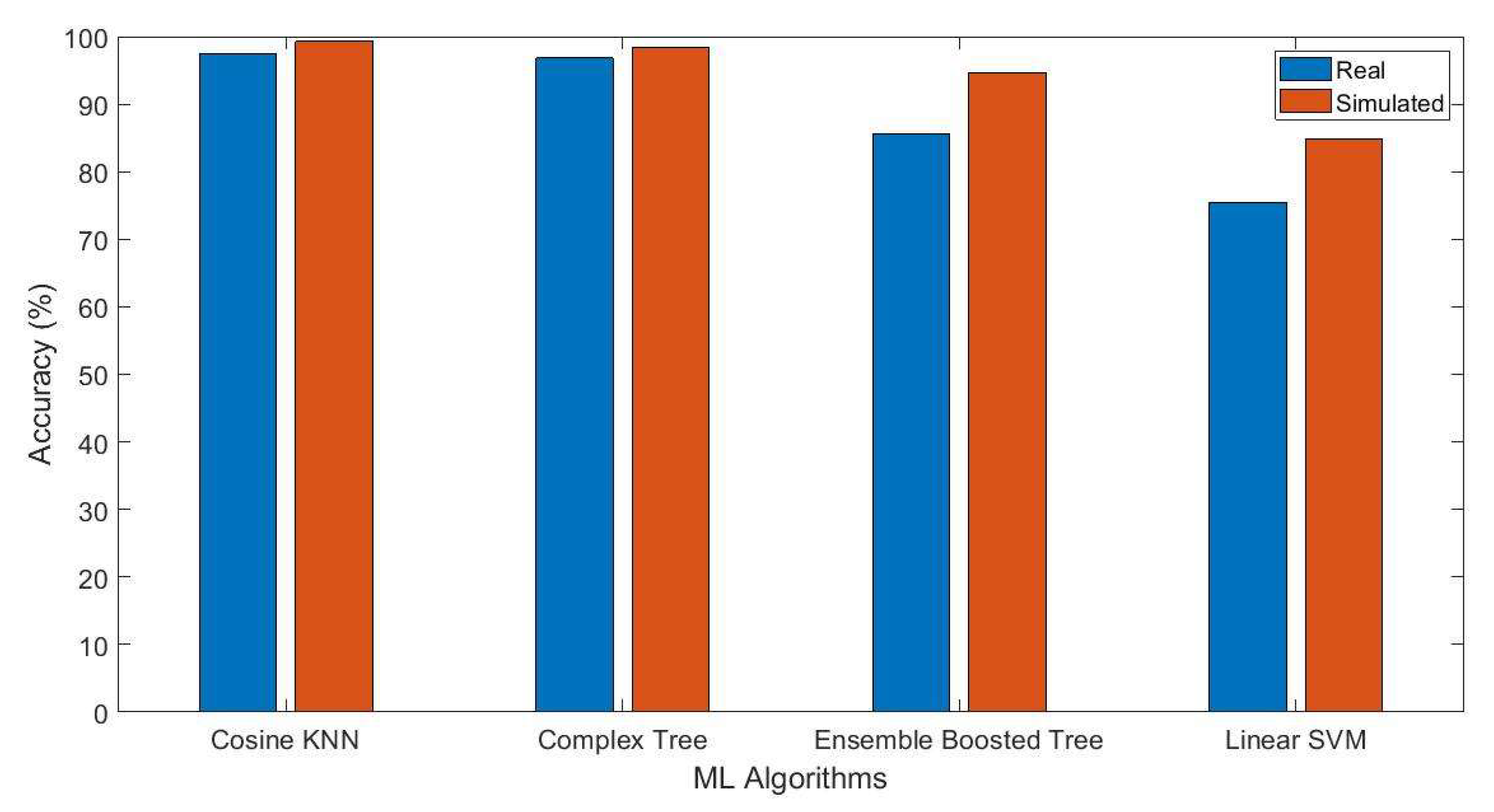
| Cosine KNN | 97.5 | ~2200 | 306.35 | 99.3 | ~500 | 2583.60 |
| Complex Tree | 96.8 | ~410,000 | 11.16 | 98.4 | ~86,000 | 140.77 |
| Ensemble Boosted Tree | 85.6 | ~80,000 | 390.58 | 94.7 | ~44,000 | 2897.90 |
| Linear SVM | 75.5 | ~98,000 | 219.75 | 84.9 | ~32,000 | 1184.90 |
Publisher’s Note: MDPI stays neutral with regard to jurisdictional claims in published maps and institutional affiliations. |
© 2021 by the authors. Licensee MDPI, Basel, Switzerland. This article is an open access article distributed under the terms and conditions of the Creative Commons Attribution (CC BY) license (https://creativecommons.org/licenses/by/4.0/).
Share and Cite
Rehman, M.; Shah, R.A.; Khan, M.B.; Shah, S.A.; AbuAli, N.A.; Yang, X.; Alomainy, A.; Imran, M.A.; Abbasi, Q.H. Improving Machine Learning Classification Accuracy for Breathing Abnormalities by Enhancing Dataset. Sensors 2021, 21, 6750. https://doi.org/10.3390/s21206750
Rehman M, Shah RA, Khan MB, Shah SA, AbuAli NA, Yang X, Alomainy A, Imran MA, Abbasi QH. Improving Machine Learning Classification Accuracy for Breathing Abnormalities by Enhancing Dataset. Sensors. 2021; 21(20):6750. https://doi.org/10.3390/s21206750
Chicago/Turabian StyleRehman, Mubashir, Raza Ali Shah, Muhammad Bilal Khan, Syed Aziz Shah, Najah Abed AbuAli, Xiaodong Yang, Akram Alomainy, Muhmmad Ali Imran, and Qammer H. Abbasi. 2021. "Improving Machine Learning Classification Accuracy for Breathing Abnormalities by Enhancing Dataset" Sensors 21, no. 20: 6750. https://doi.org/10.3390/s21206750
APA StyleRehman, M., Shah, R. A., Khan, M. B., Shah, S. A., AbuAli, N. A., Yang, X., Alomainy, A., Imran, M. A., & Abbasi, Q. H. (2021). Improving Machine Learning Classification Accuracy for Breathing Abnormalities by Enhancing Dataset. Sensors, 21(20), 6750. https://doi.org/10.3390/s21206750