Control of Dynamic Positioning System with Disturbance Observer for Autonomous Marine Surface Vessels

Abstract

The main goal of the research is to design an efficient controller for a dynamic positioning system for autonomous surface ships using the backstepping technique for the case of full-state feedback in the presence of unknown external disturbances. The obtained control commands are distributed to each actuator of the overactuated vessel via unconstrained control allocation. The numerical hydrodynamic model of CyberShip I and the model of environmental disturbances are applied to simulate the operation of the ship control system using the time domain analysis. Simulation studies are presented to illustrate the effectiveness of the proposed controller and its robustness to external disturbances.

1. Introduction

Extensive development work is currently underway on the concept of the Maritime Autonomous Surface Ship (MASS), which requires new solutions in many areas: law, economics, guidance, control and navigation [1,2,3]. Automated navigation tasks require the further development of high-level control systems; in particular, with respect to such issues as path planning and collision avoidance [4,5,6,7,8,9,10,11,12,13,14,15]. However, the basic issue in the research on developing autonomous marine surface vessels is motion control. Model-based control is used to steer and dynamically position the ship. This type of determining control algorithm became the most common approach in the beginning of the 1960s, when such techniques as the Linear Quadratic-Gaussian (LQG) and other approaches determined in the state space were used. The models used in the design of model-based control systems depend on control objectives. These targets can be roughly divided into low-speed positioning and high-speed steering [16]. The first target, called dynamic positioning (DP), involves station keeping, position mooring and dynamic tracking control at low speed [17,18,19,20,21]. High-speed steering includes automatic heading control [22,23,24,25,26,27,28,29,30], high speed position tracking [31,32,33,34,35,36], path following [37,38,39,40], roll motion control [41,42,43] and formation control [44,45].

In view of the maneuvering difficulties caused by the weight of a ship, it is not an easy task to improve the quality of navigation, especially for ships moving at low speed (called dynamic positioning). Designing an efficient dynamic positioning (DP) system for a marine vessel is a challenging practical problem. The performance and robustness of the DP system is essential for the success of the mission. In dynamic positioning systems, the main goal is to keep the marine vessel in a steady position and at a constant heading (direction) in the horizontal plane or to follow the target trajectory using only hull-mounted thrusters. The first generation of dynamic positioning systems comes from the early 1960s, when drilling began to be performed at very great depths. The first vessel equipped with a dynamic positioning system was Eureka, owned by Shell Oil Company, which entered into operation in 1961 [46]. Currently, dynamic positioning systems are used on various types of ships to perform many marine tasks, such as hydrographic surveys, marine construction, wreck research and geodesy. In the offshore oil and gas industry, many tasks can only be performed with the assistance of DP systems. This refers to the operation of service vessels, rigs and drilling vessels, shuttle tankers, cable and pipe laying units and floating production storage and offloading (FPSO) units.

The first implemented dynamic positioning systems made use of PID (Proportional–Integral–Derivative) controllers. To counteract the excessive activity of thrusts associated with wave-caused hull motion, the controllers used cut-off filters in a cascade arrangement with low-pass filters [47]. The improvement in the quality of control system operation took place after the application of more advanced control techniques based on the optimal control theory and the Kalman filter theory [48,49,50,51]. The major disadvantage of this approach was that the kinetic equations of motion had to be linearized for certain conditions. For each linearized equation, new gains were computed for the Kalman filter and for coupling, and then these gains were modified online by gain scheduling. In the 1990s, introducing nonlinear observers and feedback control theory to the designs of dynamic positioning systems resulted in the removal of assumptions related to linearization [52,53,54].

The further development of control algorithms used in dynamic positioning systems was associated with the emergence of alternative control strategies such as robust control [55,56,57,58,59,60,61,62,63], modal control [64,65], adaptive control [66] and model predictive control [46,67,68,69]. Other solutions for control systems were related to the developments taking place in non-linear control [70,71] using methods such as backstepping [72,73,74,75,76,77,78], dynamic surface control [79,80], active direct surface control [81], nonlinear PID control [18,82,83], port-Hamiltonian framework [84] and sliding mode control [85,86,87]. A hybrid DP system using supervisory switching control logic to change between the bank of controllers and observers was also proposed [88,89,90].

The dynamic positioning systems presented in some works applied tools used for modeling artificial intelligence, such as fuzzy systems [91,92,93,94,95,96,97], artificial neural networks [98,99,100,101,102,103] and neuro-fuzzy systems [104,105]. An overview of selected research works related to the technological progress in the design of dynamic positioning control systems was presented in [19,21].

In dynamic positioning systems, multivariable controllers usually determine the commanded forces and torque, which must then be generated by (obtained from) thrusters installed on the ship. For overactuated marine vessels, control allocation is a vital part of the DP system. Improper allocation may lead to degraded control performance, lower energy efficiency and the increased wear and tear of the actuators. There is a rich literature regarding control allocation for marine surface vessels, commonly referred to as thrust allocation [106,107,108,109,110,111,112,113,114,115,116,117,118,119,120]. In-depth reviews of the literature are given in [121,122].

A vessel operating in the ocean is subjected to disturbances caused by waves, wind and sea currents that cause the vessel to deviate from its desired position and direction. Hence, disturbance damping is one of the key problems in the design of DP control. The ocean disturbance can be divided into low-frequency (LF) disturbance caused by second-order waves, sea currents and wind and wave frequency (WF) disturbance caused by first-order waves. The low-frequency disturbance causes the ship to drift, while the wave frequency disturbance causes it to oscillate. The compensation of wave frequency disturbances would wear out the marine actuators and increase fuel consumption. On the other hand, there is no need to compensate for WF disturbances because they cause only oscillatory movements of the ship [69]. These motions should be filtered off by wave filtering algorithms from the vessel position and heading measurements before passing them to the DP control system. Several wave filtering techniques have been proposed [123,124,125,126]. Therefore, in this article, only the low-frequency components of environmental disturbances are considered in the DP control design.

The control objective in this paper is to design a ship motion control algorithm in dynamic positioning using the backstepping method with a disturbance observer of unmeasured disturbances affecting the ship’s hull.

2. Formulation of the Problem of Steering the Ship at Low Speed

The motion of a ship sailing on the water surface in the horizontal plane is analyzed in three degrees of freedom. This motion is described using two coordinate systems, limited to two dimensions: the inertial frame ($X_N$, $Y_N$) associated with the sea map and the body-fixed reference frame ($X_B$,$Y_B$) associated with the moving ship (Figure 1). Physical quantities assumed as state variables for the ship moving in the horizontal plane can be grouped into two vectors: $\mathit{\eta }={[x,y,\psi ]}^T$ and $\mathit{\nu }={[u,v,r]}^T$, where (x, y) are the coordinates of ship’s position, ψ is the ship’s heading, (u, v) are the linear velocity components of ship’s motion in the surge and sway directions, and r is the yaw rate [127].

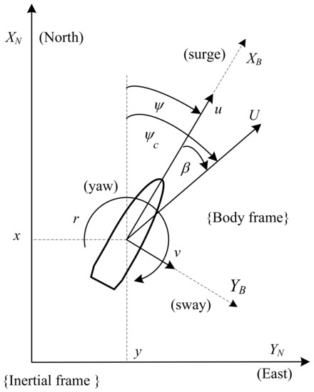
Figure 1. Coordinate systems and variables used to describe the ship motion.

The velocity vector determined in the inertial frame ($X_N$, $Y_N$) is related to that determined in the body-fixed reference frame ($X_B$, $Y_B$) by the following kinematic relationship:

$$\dot{\mathit{\eta }}=\mathit{R}\left(\psi \right)\mathit{\nu }$$

(1)

where $\mathit{R}\left(\psi \right)\in {\mathbb{R}}^{3\times 3}$ is the rotation matrix by angle $\psi$, determined from the relationship

$$\mathit{R}\left(\psi \right)=\left[\begin{array}{ccc}cos\left(\psi \right)& -sin\left(\psi \right)& 0\\ sin\left(\psi \right)& cos\left(\psi \right)& 0\\ 0& 0& 1\end{array}\right]$$

(2)

The properties of the rotation matrix given by Formula (2) are as follows

$$∥\mathit{R}\left(\psi \right)∥=1, {\mathit{R}}^{-1}\left(\psi \right)={\mathit{R}}^T\left(\psi \right), \frac{d}{dt}{\mathit{R}}^T\left(\psi \right)=-r\mathit{S}{\mathit{R}}^T\left(\psi \right)$$

(3)

where $\mathit{S}\in {\mathbb{R}}^{3\times 3}$ is the skew-symmetric matrix

$$\mathit{S}=\left[\begin{array}{ccc}0& -1& 0\\ 1& 0& 0\\ 0& 0& 0\end{array}\right], \mathit{S}=-{\mathit{S}}^T$$

(4)

The mathematical model of the dynamics of a ship sailing on the surface of the sea and ocean in the presence of environmental disturbances is described as follows [127]:

$$\mathit{M}\dot{\mathit{\nu }}+\mathit{C}\left(\mathit{\nu }\right)\mathit{\nu }+\mathit{D}\left(\mathit{\nu }\right)\mathit{\nu }=\mathit{\tau }+{\mathit{R}}^T\left(\psi \right)\mathit{b}=\mathit{\tau }+{\mathit{\tau }}_{\mathit{d}}$$

(5)

where $\mathit{M}\in {\mathbb{R}}^{3\times 3}$ is the inertia matrix, $\mathit{C}\in {\mathbb{R}}^{3\times 3}$ is the matrix of Coriolis and centripetal terms, $\mathit{D}\in {\mathbb{R}}^{3\times 3}$ is the damping matrix, and $\mathit{\tau }={[{\tau }_x,{\tau }_y,{\tau }_n]}^T$ is the input control vector consisting of the surge force ${\tau }_x$, sway force ${\tau }_y$ and yaw moment ${\tau }_n$ produced by propellers and thrusters installed in the ship’s hull. Unmodeled external low frequency (LF) forces and moments due to wind, currents and waves are connected together into an Earth-fixed constant (or slowly varying) bias term $\mathbf{b}\left(t\right)={[b_1\left(t\right),b_2\left(t\right),b_3\left(t\right)]}^T$. Here, it is assumed that the changing rate of the bias is bounded,

$$\parallel \dot{\mathit{b}}\left(t\right)\parallel \le C_d<\infty$$

(6)

where $C_d$ is a nonnegative constant. The above assumption is reasonable because the environmental energy applied to the vessel is limited.

In Equation (5), ${\mathit{\tau }}_{\mathit{d}}$ represents external disturbances acting on the vessel in the body-fixed reference frame, given as

$${\mathit{\tau }}_{\mathit{d}}={\mathit{R}}^T\left(\psi \right)\mathit{b}$$

The inertia matrix $\mathit{M}\in {\mathbb{R}}^{3\times 3}$, which includes the hydrodynamic added inertia, can be written as [127]

$$\mathit{M}=\left[\begin{array}{ccc}{m}_{11}& 0& 0\\ 0& m_{22}& m_{23}\\ 0& m_{32}& m_{33}\end{array}\right]=\left[\begin{array}{ccc}m-X_{\dot{u}}& 0& 0\\ 0& m-Y_{\dot{v}}& m{x}_G-Y_{\dot{r}}\\ 0& m{x}_G-N_{\dot{v}}& I_z-N_{\dot{r}}\end{array}\right]$$

(7)

where m is the vessel mass, $I_z$ is the moment of inertia about the fixed z-axis of the vessel, and $X_{\dot{u}}$, $Y_{\dot{v}}$, $Y_{\dot{r}}$, $N_{\dot{v}}$ and $N_{\dot{r}}$ are hydrodynamic derivatives. Zero-frequency masses are added to the surge, sway and yaw due to accelerations along the relevant axes. For control applications, which are restricted to LF motions, the wave frequency independence of the added inertia (zero wave frequency) can be assumed. This implies that $\dot{\mathit{M}}=0$.

The matrix of Coriolis and centripetal terms has the form

$$\mathit{C}=\left[\begin{array}{ccc}0& 0& -m_{22}v-m_{23}r\\ 0& 0& m_{11}u\\ m_{22}v+m_{23}r& -m_{11}u& 0\end{array}\right]$$

(8)

For a straight-line stable vessel, $\mathit{D}\in {\mathbb{R}}^{3\times 3}$ is a positive damping matrix due to linear wave drift and laminar skin friction. The linear damping matrix is defined as [127]

$$\mathit{D}=\left[\begin{array}{ccc}-X_u& 0& 0\\ 0& -Y_v& -Y_r\\ 0& -N_v& -N_r\end{array}\right]$$

(9)

3. Control Algorithms in the Dynamic Positioning System

The control objective in this paper is to design a DP control system for a ship with unknown time-varying disturbances, so that the vessel’s actual position (x, y) and heading converge to the desired values ${\mathit{\eta }}_{\mathit{d}}={[x_d,y_d,{\psi }_d]}^T$.

Assumption 1.

The desired smooth reference signal ${\mathit{\eta }}_{\mathit{d}}$ is bounded and has bounded first ${\dot{\mathit{\eta }}}_{\mathit{d}}$ and second ${\ddot{\mathit{\eta }}}_{\mathit{d}}$ derivatives. This means that the functions describing the ship’s position and direction, as well as their derivatives of the first and second order, are limited.

The considered movement of the vessel is executed at low speed in the system shown in Figure 2. The input to this control system is the vector ${\mathit{\eta }}_{\mathit{r}}$ with reference coordinates of the ship’s position and direction. The smooth and bounded desired trajectories ${\mathit{\eta }}_{\mathit{d}}$ with their first ${\dot{\mathit{\eta }}}_{\mathit{d}}$ and second-order ${\ddot{\mathit{\eta }}}_{\mathit{d}}$ derivatives needed for the controller were generated by a second-order filter:

$$G_{fi}\left(s\right)=\frac{{\omega }_{ni}^2}{s^2+2{\zeta }_i{\omega }_{ni}s+{\omega }_{ni}^2} i=1,2,3.$$

(10)

where the reference ${\mathit{\eta }}_{\mathit{r}}$ is the operator input, ${\zeta }_i$ is the relative damping ratio, and ${\omega }_{ni}$ is the natural frequency. Notice that

$$\underset{t\to \infty }{lim}{\mathit{\eta }}_d\left(t\right)={\mathit{\eta }}_r$$

(11)

and ${\dot{\mathit{\eta }}}_{\mathit{d}}$ and ${\ddot{\mathit{\eta }}}_{\mathit{d}}$ are smooth and bounded derivatives for steps in ${\mathit{\eta }}_{\mathit{r}}$.

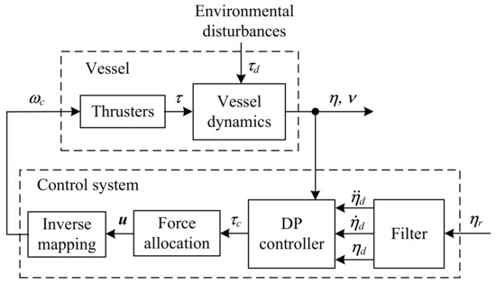
Figure 2. Block diagram of dynamic positioning control system.

The vessel is assumed to be overactuated. The trajectory of motion of such a vessel depends on the operation of all actuators installed in its hull. The controller’s task is to determine the forces and moments to be applied to the ship’s hull. This also requires the use of an appropriate system for the distribution of forces and torque determined by the controller.

3.1. Backstepping Method with Disturbance Observer

The control algorithm used in the dynamic positioning system was derived using the backstepping method and assuming that the entire plant state vector is known. The vector of control forces ${\mathit{\tau }}_c\left(t\right)$ was designed in such a way as to ensure that the state variables in vectors $\mathit{\eta }\left(t\right)$ and $\mathit{\nu }\left(t\right)$ remain constrained and that the position and course are asymptotically convergent to their set constant values $\mathit{\eta }\left(t\right)\to {\mathit{\eta }}_d\left(t\right)$ with $\mathit{\nu }\left(t\right)\approx 0$ for $t\ge 0$. The classic method of backstepping is described in [72]. The desired signals required for control are represented by the given position and direction vector ${\mathit{\eta }}_d={[x_d,y_d,{\psi }_d]}^T$ and its first ${\dot{\mathit{\eta }}}_d$ and second ${\ddot{\mathit{\eta }}}_d$ derivatives. It is assumed that all desired signals related to the ship position ($x_d$, $y_d$) and heading ${\psi }_d$ are limited.

The control deviations related to the given position and direction vector ${\mathit{\eta }}_d$ and the velocity vector $\mathit{\nu }$ were defined as

$${\mathit{z}}_1=\mathit{\eta }-{\mathit{\eta }}_d$$

(12)

$${\mathit{z}}_2=\mathit{\nu }-{\mathit{\vartheta }}_1$$

(13)

where ${\mathit{\vartheta }}_1\in {\mathbb{R}}^3$ is the stabilizing function, which is the desired virtual control. Determining the two-sided derivative from Equation (12), and substituting relation (1) and that determined from Equation (13) into this derivative, we obtain

$${\dot{\mathit{z}}}_1=\dot{\mathit{\eta }}-{\dot{\mathit{\eta }}}_d=\mathit{R}\left(\psi \right)\mathit{\nu }-{\dot{\mathit{\eta }}}_d=\mathit{R}\left(\psi \right)({\mathit{z}}_2+{\mathit{\vartheta }}_1)-{\dot{\mathit{\eta }}}_d$$

(14)

The stabilizing function ${\mathit{\vartheta }}_1$ was assumed as

$${\mathit{\vartheta }}_1={\mathit{R}}^{-1}\left(\psi \right)(-{\mathit{K}}_1{\mathit{z}}_1+{\dot{\mathit{\eta }}}_d)$$

(15)

where ${\mathit{K}}_1={\mathit{K}}_1^T>0$ is the diagonal positive definite gain matrix. The stabilizing function ${\mathit{\vartheta }}_1$, which is the desired virtual control for vector $\mathit{\nu }$, was determined in relation to the Lyapunov function in the form $V_1=0.5{\mathit{z}}_1^T{\mathit{z}}_2$. Substituting relation (15) into Equation (14) and using the relation $\mathit{R}\left(\psi \right){\mathit{R}}^{-1}\left(\psi \right)=\mathit{I}$, we obtain

$${\dot{\mathit{z}}}_1=-{\mathit{K}}_1{\mathit{z}}_1+\mathit{R}\left(\psi \right){\mathit{z}}_2$$

(16)

Determining the two-sided derivative from Equation (13) and substituting the relation determined from Equation (5) into it, we obtain

$${\dot{\mathit{z}}}_2=\dot{\mathit{\nu }}-{\dot{\mathit{\vartheta }}}_1={\mathit{M}}^{-1}[-\mathit{C}\left(\mathit{\nu }\right)\mathit{\nu }-\mathit{D}\mathit{\nu }+\mathit{\tau }+{\mathit{R}}^T\left(\psi \right)\mathit{b}]-{\dot{\mathit{\vartheta }}}_1$$

(17)

where $\dot{{\mathit{\vartheta }}_1}$, determined based on Equation (15), takes the form

$${\dot{\mathit{\vartheta }}}_1=-r\mathit{S}{\mathit{R}}^T\left(\psi \right)(-{\mathit{K}}_1{\mathit{z}}_1+{\dot{\mathit{\eta }}}_d)+{\mathit{R}}^T\left(\psi \right)(-{\mathit{K}}_1{\dot{\mathit{z}}}_1+{\ddot{\mathit{\eta }}}_d)$$

(18)

With regard to the Lyapunov function in the form $V_2=V_1+0.5{\mathit{z}}_2^T\mathit{M}{\mathit{z}}_2$, the following control law was adopted:

$${\mathit{\tau }}_c=\mathit{C}\left(\mathit{\nu }\right)\mathit{\nu }+\mathit{D}\mathit{\nu }-\mathit{M}{\mathit{K}}_2{\mathit{z}}_2-\mathit{M}{\mathit{R}}^T\left(\psi \right){\mathit{z}}_1+\mathit{M}{\dot{\mathit{\vartheta }}}_1-{\mathit{R}}^T\left(\psi \right)\widehat{\mathit{b}}$$

(19)

where ${\mathit{K}}_2={\mathit{K}}_2^T>0$ is the positively defined gain matrix, and the vector $\widehat{\mathit{b}}$ contains estimates of the parameters of the external bias term $\mathit{b}$ describing external disturbances acting on the vessel. The disturbance observer for the bias vector $\mathit{b}$ was constructed using the exponential convergent observer from [128]

$$\widehat{\mathit{b}}=\mathit{R}\left(\psi \right)[\mathit{\theta }+{\mathit{K}}_0\mathit{M}\mathit{\nu }]$$

(20)

$$\dot{\mathit{\theta }}=-{\mathit{K}}_0\mathit{\theta }-{\mathit{K}}_0[-\mathit{C}\left(\mathit{\nu }\right)\mathit{\nu }-\mathit{D}\mathit{\nu }+{\mathit{\tau }}_c+{\mathit{K}}_0\mathit{M}\mathit{\nu }]$$

(21)

where $\widehat{\mathit{b}}\left(t\right)={[{\widehat{b}}_1\left(t\right),{\widehat{b}}_2\left(t\right),{\widehat{b}}_3\left(t\right)]}^T$ is the estimate of the bias term, $K_0$ is the 3 × 3 positive definite symmetric observer gain matrix, and $\mathit{\theta }$ is the 3 × 1 intermediate auxiliary vector.

Considering the ship dynamics given by Formula (5) and the desired trajectory ${\mathit{\eta }}_d$, which is smooth and limited, the information about all ship states $\mathit{x}$ is provided. In this case, the control law is described by Formula (19). The law of adaptation of unknown parameters related to environmental disturbances is described by Formula (20) and has zero values as initial conditions. The entered design parameters ${\mathit{K}}_0={\mathit{K}}_0^T>0$, ${\mathit{K}}_1={\mathit{K}}_1^T>0$, ${\mathit{K}}_2={\mathit{K}}_2^T>0$ are positively defined. These conditions mean that the entire closed control system is stable, and consequently the signals ${\mathit{z}}_1$ and ${\mathit{z}}_2$ have finite values.

3.2. Nonlinear PID Controller

The controller used to compare the obtained results of simulation tests was the nonlinear PID controller for DP systems, described in detail in [18]. The algorithm of this controller is given by the formula

$${\mathit{\tau }}_{PID}=\mathit{M}{\mathit{R}}^{-1}\left(\psi \right)[{\dot{\mathit{\nu }}}_d-{\mathit{K}}_P{\mathit{\eta }}_e-{\mathit{K}}_I{\mathit{\xi }}_e-{\mathit{K}}_D{\mathit{\nu }}_e-{\dot{\psi }}_e\mathit{R}\left(\psi \right)\mathit{S}\mathit{\nu }]+\mathit{C}\left(\mathit{\nu }\right)\mathit{\nu }+\mathit{D}\mathit{\nu }$$

(22)

where $\mathit{R}$ is the rotation matrix (2), $\mathit{S}$ is the skew-symmetric matrix (4), $\mathit{M}$ is the inertia matrix (7), $\mathit{C}\left(\mathit{\nu }\right)$ is the Coriolis and centripetal matrix (8), $\mathit{D}$ is the matrix of hydrodynamic damping (9), and ${\mathit{K}}_P$, ${\mathit{K}}_I$ and ${\mathit{K}}_D$ are the matrix gains of the nonlinear PID controller. In this algorithm, the position and orientation errors ${\mathit{\eta }}_e$ are determined in the inertial frame ($X_N$, $Y_N$), while the velocity error ${\mathit{\nu }}_e$ and the acceleration error ${\dot{\mathit{\nu }}}_e$ are determined in the body-fixed reference frame ($X_B$, $Y_B$) associated with the moving ship

$${\mathit{\eta }}_e=\mathit{\eta }-{\mathit{\eta }}_d$$

(23)

$${\mathit{\nu }}_e=\mathit{\nu }-{\mathit{\nu }}_d=\mathit{\nu }-{\mathit{R}}^T\left(\psi \right){\dot{\mathit{\eta }}}_d$$

(24)

$${\dot{\mathit{\nu }}}_e=\dot{\mathit{\nu }}-{\dot{\mathit{\nu }}}_d=\dot{\mathit{\nu }}-\dot{{\mathit{\psi }}_e}{\mathit{S}}^T{\mathit{R}}^T\left(\psi \right){\dot{\mathit{\eta }}}_d-{\mathit{R}}^T\left(\psi \right){\ddot{\mathit{\eta }}}_d$$

(25)

$${\dot{\psi }}_e=\dot{\psi }-{\dot{\psi }}_d=r-{\dot{\psi }}_d$$

(26)

$${\dot{\mathit{\xi }}}_e={\mathit{\eta }}_e$$

(27)

The gain matrices of the nonlinear PID controller are positively defined: ${\mathit{K}}_P={\mathit{K}}_P^T>0$, ${\mathit{K}}_I={\mathit{K}}_I^T>0$, and ${\mathit{K}}_D={\mathit{K}}_D^T>0$.

3.3. Unconstrained Control Allocation

The vectors ${\mathit{\tau }}_c$ or ${\mathit{\tau }}_{PID}$ of the desired forces and moments determined by the DP controllers were divided by the allocation system into the commanded values for the actuators installed in the ship’s hull (Figure 2). It is assumed that the ship is fitted with q propulsion devices located at positions

$$\mathit{l}\left(i\right)=[l_{i,x},l_{i,y}]$$

(28)

where $l_{i,x}$, $l_{i,y}$ are the distances of the propulsion devices from the origin of the coordinate system associated with the moving ship. These devices can provide the thrust force $T_i$ in the direction defined by the angle ${\alpha }_i$. The azimuth thrusters have the angle ${\alpha }_i$ fixed in a certain direction and produce the following contributions to the generalized forces acting on the ship [120]:

$$T_{xi}=T_{i}cos\left({\alpha }_i\right)$$

(29)

$$T_{yi}=T_{i}sin\left({\alpha }_i\right)$$

(30)

$$N\left(i\right)=T_i{L}_i$$

(31)

where $L_i=l_{i,x}sin\left({\alpha }_i\right)-l_{i,y}cos\left({\alpha }_i\right)$.

The sum of the generalized forces acting on the ship’s hull from all installed propellers is given by the formula

$${\mathit{\tau }}_c=\mathit{B}\mathit{u}$$

(32)

where

$$\mathit{B}=\left[\begin{array}{cccc}cos\left({\alpha }_1\right)& cos\left({\alpha }_2\right)& \cdots & cos\left({\alpha }_q\right)\\ sin\left({\alpha }_1\right)& sin\left({\alpha }_2\right)& \cdots & sin\left({\alpha }_q\right)\\ L_1& L_2& \cdots & L_q\end{array}\right]$$

(33)

In Formula (32), ${\mathit{\tau }}_c\in {\mathbb{R}}^3$ is the input control vector, and $\mathit{u}\in {\mathbb{R}}^q$ is the vector of the set forces for each actuator.

In control allocation, the optimization of a given quality indicator, such as the minimum energy expenditure for control, is often performed. The problem of optimal control allocation has been considered as a minimization problem with constrained equality [122]

$$\underset{\mathit{u}}{min}{\mathit{u}}^T\mathit{W}\mathit{u} \mathrm{i}\mathrm{n} \mathrm{r}\mathrm{e}\mathrm{l}\mathrm{a}\mathrm{t}\mathrm{i}\mathrm{o}\mathrm{n} \mathrm{t}\mathrm{o} \mathit{B}\mathit{u}={\mathit{\tau }}_c$$

(34)

where $\mathit{W}\in {\mathbb{R}}^{qxq}$ is the weight matrix.

Considering the Lagrangian function, the formulated optimization problem (34) can be written as the unlimited minimization problem in the form

$$L(\mathit{u},\mathit{\lambda })={\mathit{u}}^T\mathit{W}\mathit{u}+{\mathit{\lambda }}^T(-\mathit{B}\mathit{u}+{\mathit{\tau }}_c)$$

(35)

where $\mathit{\lambda }\in {\mathbb{R}}^3$ is the vector containing Lagrange multipliers. The Karush–Kuhn–Tucker (KKT) conditions provide the necessary conditions for the optimal solution

$$\frac{\partial L(\mathit{u},\mathit{\lambda })}{d\mathit{u}}=2\mathit{W}\mathit{u}-{\mathit{B}}^T\mathit{\lambda }=0 \to \mathit{u}=\frac{1}{2}{\mathit{W}}^{-1}{\mathit{B}}^T\mathit{\lambda }$$

(36)

$$\frac{\partial L(\mathit{u},\mathit{\lambda })}{d\mathit{u}}=-\mathit{B}\mathit{u}+{\mathit{\tau }}_c=0 \to \mathit{B}\mathit{u}={\mathit{\tau }}_c$$

(37)

After solving the system of Equations (36) and (37), the sought vector of Lagrange multipliers is obtained as

$$\mathit{\lambda }=2{\left({\mathit{B}\mathit{W}}^{-1}{\mathit{B}}^T\right)}^{-1}{\mathit{\tau }}_c$$

(38)

Substituting Equation (38) to (36) gives

$$\mathit{u}={\mathit{W}}^{-1}{\mathit{B}}^T{\left({\mathit{B}\mathit{W}}^{-1}{\mathit{B}}^T\right)}^{-1}{\mathit{\tau }}_c$$

(39)

When the matrix ${\mathit{B}\mathit{W}}^{-1}{\mathit{B}}^T$ is non-singular, the optimization problem (34) can be solved by finding the solution to the linear equation described by Formula (39).

4. Simulations

To demonstrate the effectiveness of the developed control algorithm, selected simulation tests were carried out with the dynamic positioning system.

4.1. Ship Model

The mathematical model of CyberShip I was chosen as the ship model for determining and testing the control system at low speed. This model was developed in the Department of Engineering Cybernetics, Norwegian University of Science and Technology (NTNU), Trondheim, Norway. The physical model of this ship sails in the Marine Cybernetics Laboratory, NTNU (http://www.ntnu.edu/imt/lab/cybernetics (accessed on 10 September 2021)).

CyberShip I is a thruster-controlled model of an offshore supply vessel, made at a scale of 1:70. Its mass is m = 17.6 kg with length L = 1.19 m. The centre of gravity is located at $x_G=-0.04$ m aft of the midship. This point was assumed to be the origin of the body-fixed coordinate system. In its general form, the mathematical model of CyberShip I is described by Formula (5). Based on hydrodynamic methods and system identification, model parameters for 3 degrees of CyberShip I freedom of motion were found [17,129,130]. The inertia matrix including zero-frequency hydrodynamic added inertia is as follows:

$$\mathit{M}=\left[\begin{array}{ccc}19.0& 0& 0\\ 0& 35.2& -0.704\\ 0& -0.704& 1.98\end{array}\right]$$

(40)

The matrix of linear interactions related to hydrodynamic damping is defined as

$$\mathit{D}=\left[\begin{array}{ccc}4& 0& 0\\ 0& 6& 0\\ 0& 0& 1\end{array}\right]$$

(41)

In real-time control systems, the mathematical model of the plant does not fully reflect its dynamics. To bring the simulation tests closer to the conditions in real-time control systems, new parameters of matrices $\mathit{M}$ and $\mathit{D}$ were determined for the model of ship dynamics. In Figure 2, the model of the plant is included in a block labeled “vessel dynamics”. The principle of determining new parameter values was based on the values contained in the model described by matrices (40) and (41). The correction values Δ were determined randomly and could at most amount to ±50% of the parameter values included in these matrices. In this way, the following matrix values were determined:

$${\mathit{M}}_{vessel}=\left[\begin{array}{ccc}26.4272& 0& 0\\ 0& 51.3671& -0.7372\\ 0& -0.7372& 1.2645\end{array}\right]$$

(42)

$${\mathit{D}}_{vessel}=\left[\begin{array}{ccc}4.3411& 0& 0\\ 0& 6.2983& 0\\ 0& 0& 1.2577\end{array}\right]$$

(43)

The model of Cybership I is equipped with four rpm-controlled thrusters with independently controllable azimuth angles ${\alpha }_i$. The thrusters are controlled by the rotational speed ${\omega }_i$. Figure 3 shows the location of the actuators installed on CyberShip I.

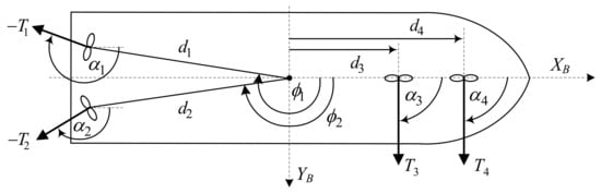
Figure 3. Thruster configuration on CyberShip I: α₁ = − 43°, α₂ = − 43°, α₃ = α₄ − 90°, ϕ₁ = 186°, ϕ₂ = 174°, ϕ₃ = ϕ₄, = 0°, d₁ = d₂ = 0.4391 m, d₃ = 0.34 m, d₄ = 0.46 m.

The forces and moment generated by the thrusters are given by the formula

$${\mathit{\tau }}_c=\mathit{B}\left(\alpha \right)\mathit{T}$$

(44)

where $\mathit{B}\in {\mathbb{R}}^{3\times 4}$ is the thruster configuration matrix described by Formula (33), in which

$$\begin{array}{c}{l}_{i,x}=d_{i}cos\left({\varphi }_i\right)\\ l_{i,y}=d_{i}sin\left({\varphi }_i\right)\end{array} i\in [1,4]$$

(45)

while the components of the thrust vector of thrusters $\mathit{T}\in {\mathbb{R}}^4$ are described by the formula

$$T_i=\left\{\begin{array}{cc}{k}_{iT}{\omega }_i^2& {\omega }_i\ge 0\\ k_{iT}\left|{\omega }_i\right|{\omega }_i& {\omega }_i<0\end{array} i\in [1,4]\right.$$

(46)

where $k_{1T}=k_{2T}=k_{4T}=3.125·{10}^{-3}$, $k_{3T}=2.5·{10}^{-4}$. The thrusts generated by the azimuth thrusters are [131]

$${\mathit{T}}_{\mathrm{m}\mathrm{a}\mathrm{x}}=-{\mathit{T}}_{\mathrm{m}\mathrm{i}\mathrm{n}}={\left[0.8 0.8 0.1 0.8\right]}^T$$

(47)

The inverse characteristics of the thrusters, determined based on Formula (46), have the form

$${\omega }_i=\mathrm{s}\mathrm{g}\mathrm{n}\left(T_i\right)\sqrt{\frac{|T_i|}{k_{iT}}} i\in [1,4]$$

(48)

The limits imposed on the rotational speeds of thrusters were determined based on Formula (48) and related parameters as

$${\mathit{\omega }}_{\mathrm{m}\mathrm{a}\mathrm{x}}=-{\mathit{\omega }}_{\mathrm{m}\mathrm{i}\mathrm{n}}={\left[16 16 20 16\right]}^T$$

(49)

After taking the related data, the configuration matrix described by Formula (33) takes the form

$$\mathit{B}={\left[\begin{array}{cccc}\hfill 0.7314& \hfill 0.7314& \hfill 0& \hfill 0\\ \hfill -0.6820& \hfill 0.6820& \hfill 1& \hfill 1\\ \hfill 0.3314& \hfill -0.3314& \hfill 0.34& \hfill 0.46\end{array}\right]}^T$$

(50)

The limits imposed on the values of forces and moments generated by the thrusters are as follows:

$${\mathit{\tau }}_{\mathrm{m}\mathrm{a}\mathrm{x}}=-{\mathit{\tau }}_{\mathrm{m}\mathrm{i}\mathrm{n}}={\mathit{B}\mathit{T}}_{\mathrm{m}\mathrm{a}\mathrm{x}}={\left[1.17 0.9 0.4\right]}^T$$

(51)

4.2. Parameters of Control Systems

The mathematical model of the control system is shown in Figure 2. Here, the vessel model marked as “vessel dynamics” and described by Formula (5) contains the matrix coefficients $\mathit{M}$ and $\mathit{D}$, given by Formulas (42) and (43), respectively. The coefficients of matrix $\mathit{C}$ are determined from Formula (8). The tested control algorithms described by Formulas (19) and (22) also contain matrices $\mathit{M}$, $\mathit{C}$ and $\mathit{D}$. In this case, the values of coefficients described by Formulas (40) and (41) were adopted. Other parameters of the controller determined by the backstepping method (19) are as follows: ${\mathit{K}}_0$ = diag {2, 2, 2}, ${\mathit{K}}_1$ = diag {0.05, 0.05, 0.05}, ${\mathit{K}}_2$ = diag {1, 1, 1}. The parameters of the gain matrices ${\mathit{K}}_P$, ${\mathit{K}}_I$ and ${\mathit{K}}_D$ for the nonlinear PID controller (22) were determined based on the mathematical model of Cybership I, given by Formulas (40) and (41), using the Particle Swarm Optimization algorithm and assuming no external disturbances. In this way, the following parameters were obtained for the nonlinear PID controller: ${\mathit{K}}_P$ = diag {1.25, 7.4, 9.95}, ${\mathit{K}}_I$ = diag {0.035, 0.343, 1.0}, ${\mathit{K}}_D$ = diag {3.57, 6.88, 6.06}.

The parameters of the reference model (10) were ${\zeta }_i$ = 1, ${\omega }_{ni}$ = 0.08, where i = 1, 2, 3. The maximum values in Formulas (19) and (22) were imposed as limits on the control signal generated by the DP controllers (51). In the control allocation system, the values of the weight matrix $\mathit{W}$ were $\mathit{W}$ = diag {1, 1, 10, 1}.

The analyzed case concerns dynamic positioning in which the vessel keeps a constant initial position ${\mathit{\eta }}_B$ = [1 m, 1 m, 45°]^T for 100 s, then moves to the new position ${\mathit{\eta }}_E$ = [2 m, 1.2 m, °]^T, to maintain it for the next period of time. The initial conditions of the vessel variable vector were $\mathit{\eta }$ = [1 m, 1 m, 45°]^T, $\mathit{\nu }$ = [0 m/s, 0 m/s, 0°/s]^T. For the disturbance observer, the initial conditions were $\widehat{\mathit{b}}$ = [0 N, 0 N, 0 Nm]^T.

4.3. Case 1—Constant Disturbances

The first analyzed case concerns the situation in which environmental disturbances remained constant in the entire analyzed range of dynamic position control:

$$\mathit{b}\left(t\right)={\left[0.35 \mathrm{N} 0.35 \mathrm{N} 0.35\mathrm{N}\mathrm{m}\right]}^T$$

(52)

The simulation test results obtained for this case are shown in Figure 4, Figure 5, Figure 6, Figure 7, Figure 8, Figure 9 and Figure 10. The time histories of environmental disturbances $\mathit{b}$ and their estimates $\widehat{\mathit{b}}$ are shown in Figure 4, from which it can be seen that in steady states the disturbance estimates coincide. There are, however, two transients: the first after switching on the control and the second after starting to change the vessel position. The zoomed time segments representing transient states are shown in Figure 5. The first transient lasts about 8 s, while the second is longer and lasts about 80 s. In this latter transient state, the deviations from the real value are very small. Figure 6 shows that the proposed controller is able to follow the desired reference trajectory. The time histories showing the desired and actual ship positions (x, y) and courses $\psi$ can follow the desired trajectory ${\mathit{\eta }}_d={[x_d,y_d,{\psi }_d]}^T$ with good precision. The deviations from the desired values are shown in Figure 7. It is noteworthy that greater values of deviations were recorded in the initial period of time and during the stabilization of the set exchange rate. This is mainly due to the low power of the actuators installed in the CyberShip I hull to generate the angular moment ${\tau }_n$. Figure 8 presents the time histories of ship velocity changes in the surge u, sway v and yaw r directions, while the next graphs show the time histories of other quantities occurring in the control system, such as the desired forces ${\tau }_x$, ${\tau }_y$ and moment ${\tau }_n$, which are the output signals from the controllers (Figure 9) and the commanded rotational speeds of the thrusters installed in the vessel’s hull (Figure 10).

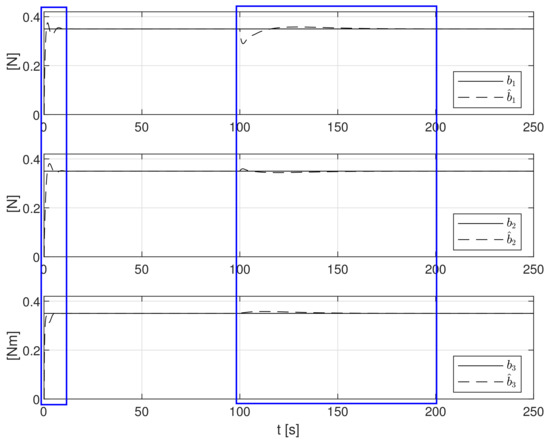
Figure 4. Constant external bias terms b₁, b₂, b₃ and their estimates ${\widehat{b}}_1$, ${\widehat{b}}_2$, ${\widehat{b}}_3$.

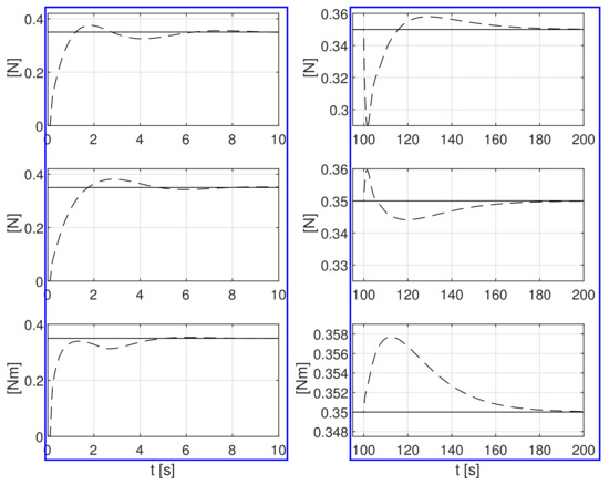
Figure 5. Zoomed partitions of constant external bias terms b₁, b₂, b₃ and their estimates ${\widehat{b}}_1$, ${\widehat{b}}_2$, ${\widehat{b}}_3$ from Figure 4.

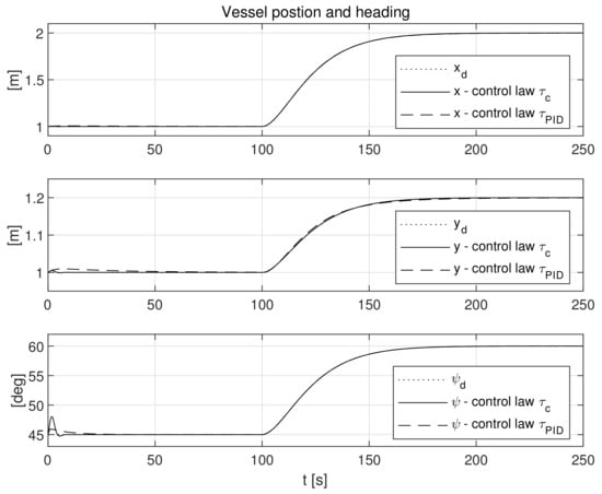
Figure 6. Vessel position (x, y) and heading (ψ) in the presence of constant environmental disturbances.

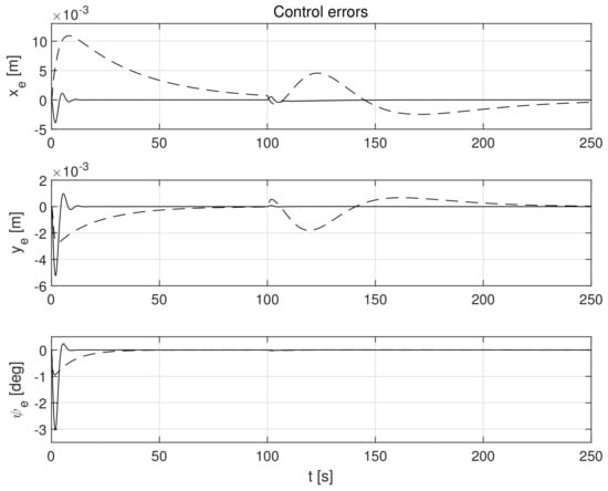
Figure 7. Errors in control systems in the presence of constant environmental disturbances: x_e, y_e-position errors, ψ_e-heading error (solid lines-control law τ_c, dotted lines-control law τ_PID).

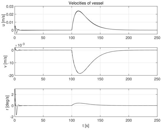
Figure 8. Velocities in control systems in the presence of constant environmental disturbances in surge (u), sway (v), and yaw (r) directions (solid lines-control law τ_c, dotted lines-control law τ_PID).

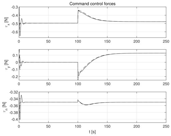
Figure 9. Command forces τ_x, τ_y and moment τ_n at outputs of controllers in the presence of constant environmental disturbances (solid lines-control law τ_c, dotted lines-control law τ_PID).

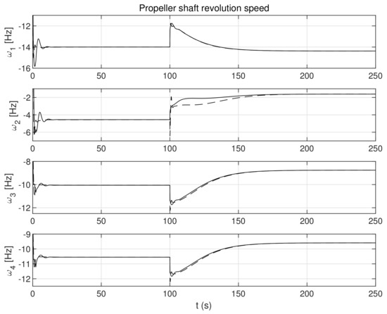
Figure 10. Command propeller shaft revolution speeds in the control systems in the presence of constant environmental disturbances (solid lines-control law τ_c, dotted lines-control law τ_PID).

4.4. Case 2—Stochastic and Time-Varying Disturbances

In the next tested case, the disturbances affecting the ship with stochastic and time-varying forces and moment described by Formula (53) were considered:

$$\mathit{b}\left(t\right)=\left[\begin{array}{c}0.4+0.05sin\left(0.035t\right)+0.1sin\left(0.025t\right)+0.1sin\left(0.045t\right) N\\ 0.3+0.3sin\left(0.05t\right) N\\ 0.2+0.025sin\left(0.01t\right)cos\left(0.03t\right) Nm\end{array}\right]$$

(53)

The simulation test results obtained for this case are shown in Figure 11, Figure 12, Figure 13, Figure 14, Figure 15, Figure 16 and Figure 17. The time histories of environmental disturbances $\mathit{b}$ and their estimates $\widehat{\mathit{b}}$ are shown in Figure 11, from which it can be seen that, in the steady states, the disturbance estimates coincide. There are, however, two transients: the first after switching on the control, and the second after starting to change the position of the vessel. The zoomed time segments representing the transient states are shown in Figure 11. The first transient lasts about 10 s, while in the second transient, small deviations are observed in estimates ${\widehat{b}}_1$ and ${\widehat{b}}_3$. There are no deviations in the estimate ${\widehat{b}}_2$. The time histories of the desired and actual ship positions (x, y) and ship course $\psi$ shown in Figure 13 follow the desired trajectory ${\mathit{\eta }}_d={[x_d,y_d,{\psi }_d]}^T$ with good precision. The deviations from the desired values are shown in Figure 14. Figure 15 presents the time histories of ship velocity changes in the surge u, sway v and yaw r directions. The next graphs show the time histories of other quantities occurring in the control system, such as the desired forces ${\tau }_x$, ${\tau }_y$ and moment ${\tau }_n$, which are the output signals from the controllers (Figure 16), and the command rotational speeds of the thrusters installed in the vessel’s hull (Figure 17).

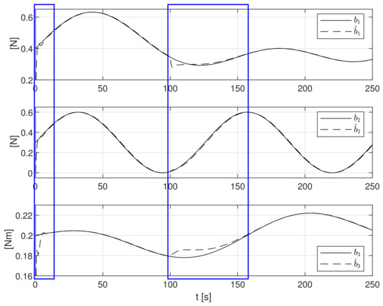
Figure 11. Stochastic and time-varying external bias terms b₁, b₂, b₃ and their estimates ${\widehat{b}}_1$, ${\widehat{b}}_2$, ${\widehat{b}}_3$.

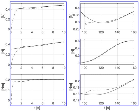
Figure 12. Zoomed partitions of constant external bias terms b₁, b₂, b₃ and their estimates ${\widehat{b}}_1$, ${\widehat{b}}_2$, ${\widehat{b}}_3$ from Figure 11.

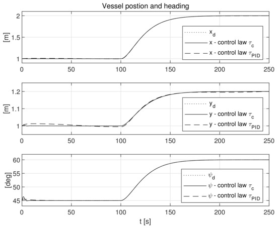
Figure 13. Vessel position (x, y) and heading (ψ) with controllers with stochastic and time-varying disturbances.

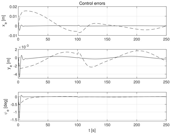
Figure 14. Errors in control systems in the presence of stochastic and time-varying disturbances: x_e, y_e-position errors, ψ_e-heading errors (solid lines-control law τ_c, dotted lines-control law τ_PID).

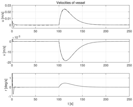
Figure 15. Velocities in control systems in the presence of stochastic and time-varying disturbances: u-surge, v-sway, r-yaw directions (solid lines-control law τ_c, dotted lines-control law τ_PID).

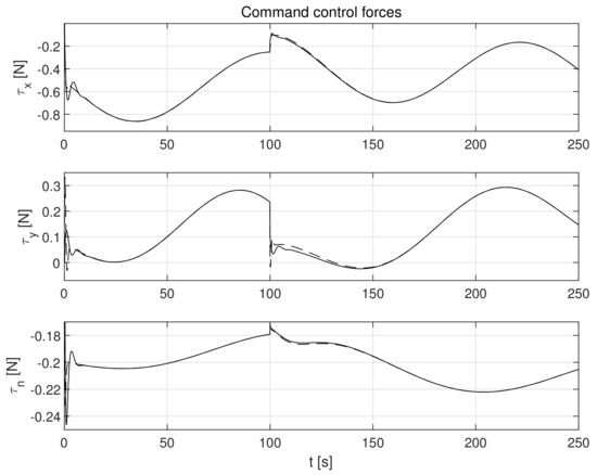
Figure 16. Command forces τ_x, τ_y and moment τ_n in control systems in the presence of of stochastic and time-varying disturbances (solid lines-control law τ_c, dotted lines-control law τ_PID).

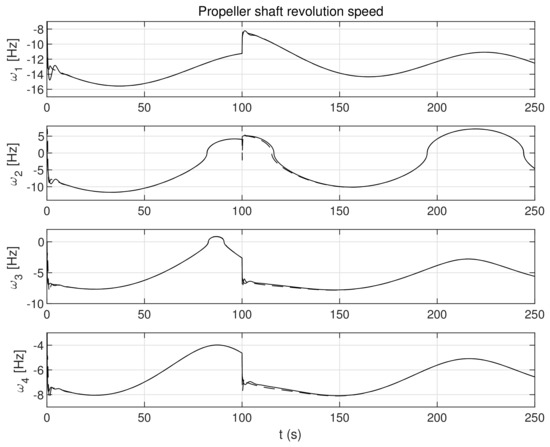
Figure 17. Command propeller shaft revolution speeds in control systems in the presence of stochastic and time-varying disturbances (solid lines-control law τ_c, dotted lines-control law τ_PID).

A quantitative comparison of the quality of the performance of the two considered controllers acting in the presence of constant and changing disturbances is given in Table 1, where $x_e=x_d-x$, $y_e=y_d-y$ are the errors between the desired and current position, ${\psi }_e={\psi }_d-\psi$ is the difference between the desired and actual heading of the vessel and $t_f$ = 250 s. The results presented in Table 1 clearly show that the controller τ_c (20) has better control quality than the nonlinear τ_PID controller (22).

Table 1. Comparison of quality performance of two control laws τ_c and τ_PID with different disturbances.

Disturbances	Constant		Stochastic and Time-Varying
Controller	τc	τPID	τc	τPID
$\underset{0}{\overset{t_f}{\int }}\left|x_e\left(t\right)\right|dt$	0.1948	6.8797	0.4237	11.7068
$\underset{0}{\overset{t_f}{\int }}\left|y_e\left(t\right)\right|dt$	0.1564	1.3406	0.6250	2.8474
$\underset{0}{\overset{t_f}{\int }}\left|{\psi }_e\left(t\right)\right|dt$	80.7763	105.9706	45.6141	80.5418

5. Discussion

Numerous institutions and universities are becoming increasingly interested in the development of control algorithms for autonomous marine surface vessels. One of the important tasks is the automation of the process of controlling the surface vessel’s motion for the entire voyage, starting from the departure port and ending at the destination port. In this case, the desired route of the system consists of a number of different-type segments, and thus it may be necessary to use different controllers at different path stages. Ship navigation on the desired route defined in the above way requires the design of a control system that is capable of executing various tasks, such as ship undocking and docking, maneuvering in the port area, movement along the desired route with transit speed and stopping on the route. Such a solution was presented in [132].

The control algorithm presented in this article is planned to be used in a multi-operational system to control the motion of a ship on those segments of the voyage route where the vessel will sail in dynamic positioning mode; i.e., in ports and very narrow navigation canals, on access routes to the port and in the maneuvers performed to reach the docking place.

6. Conclusions

The article presents a ship motion control system with a disturbance observer for the dynamic positioning of a fully actuated autonomous marine surface vessel in the presence of uncertain time-variant disturbances due to wind, waves and ocean currents. Both the Coriolis and centripetal matrix and the linear damping matrix are considered in the mathematical model of the vessel. The control strategy is introduced by the backstepping technique with a disturbance observer used to compensate for uncertainties associated with the disturbances. The simulation tests carried out on the model of a sea-going vessel have shown that the designed controller is effective in compensating for external disturbances. The proposed control system is characterized by a good quality of work both during the stabilization of the fixed position of the ship and when moving it to a new position.

The unconstrained control allocation was used to allocate the desired control to individual actuators. The applied allocation method allows for the distribution of the desired forces and moment determined by the DP controller into any number of thrusters installed in the ship’s hull with a fixed thruster, which is a non-rotatable device, and its orientation angle α cannot be changed.

References

- Shi, Y.; Shen, C.; Fang, H.; Li, H. Advanced control in marine mechatronic systems: A survey. IEEE/ASME Trans. Mechatron. 2017, 22, 1121–1131. [Google Scholar] [CrossRef]
- Liu, Z.; Zhang, Y.; Yu, X.; Yuan, C. Unmanned surface vehicles: An overview of developments and challenges. Annu. Rev. Control 2016, 41, 71–93. [Google Scholar] [CrossRef]
- Zereik, E.; Bibuli, M.; Mišković, N.; Ridao, P.; Pascoal, A. Challenges and future trends in marine robotics. Annu. Rev. Control 2018, 46, 350–368. [Google Scholar] [CrossRef]
- Rak, A.; Gierusz, W. Reinforcement learning in discrete and continuous domains applied to ship trajectory generation. Pol. Marit. Res. 2012, 19, 31–36. [Google Scholar] [CrossRef][Green Version]
- Szymak, P. Comparison of fuzzy system with neural aggregation FSNA with classical TSK fuzzy system in anti-collision problem of USV. Pol. Marit. Res. 2017, 24, 3–14. [Google Scholar] [CrossRef]
- Lazarowska, A. Comparison of discrete artificial potential field algorithm and wave-front algorithm for autonomous ship trajectory planning. IEEE Access 2020, 8, 221013–221026. [Google Scholar] [CrossRef]
- Lisowski, J.; Mohamed-Seghir, M. Comparison of computational intelligence methods based on fuzzy sets and game theory in the synthesis of safe ship control based on information from a radar ARPA system. Remote Sens. 2019, 11, 82. [Google Scholar] [CrossRef]
- Lisowski, J. Multi-criteria optimisation of multi-stage positional game of vessels. Pol. Marit. Res. 2020, 27, 46–52. [Google Scholar] [CrossRef]
- Miller, A.; Walczak, S. Maritime autonomous surface ship’s path approximation using Bézier curves. Symmetry 2020, 12, 1704. [Google Scholar] [CrossRef]
- Miller, A.; Rybczak, M.; Rak, A. Towards the autonomy: Control systems for the ship in confined and open waters. Sensors 2021, 21, 2286. [Google Scholar] [CrossRef] [PubMed]
- Song, L.; Chen, H.; Xiong, W.; Dong, Z.; Mao, P.; Xiang, Z.; Hu, K. Method of emergency collision avoidance for unmanned surface vehicle (USV) based on motion ability database. Pol. Marit. Res. 2019, 26, 55–67. [Google Scholar] [CrossRef]
- Szłapczyński, R.; Ghaemi, H. Framework of an evolutionary multi-objective optimisation method for planning a safe trajectory for a marine autonomous surface ship. Pol. Marit. Res. 2019, 26, 69–79. [Google Scholar] [CrossRef]
- Śmierzchalski, R.; Łebkowski, A. Evolutionary-Fuzzy Hybrid System of Steering the Moveable Object in Dynamic Invironment. In Proceedings of the 6th IFAC Conference Control Application in Marine Craft, Girona, Spain, 17–19 September 2003; pp. 235–240. [Google Scholar]
- Vagale, A.; Oucheikh, R.; Bye, R.T.; Osen, O.L.; Fossen, T.I. Path planning and collision avoidance for autonomous surface vehicles I: A review. J. Mar. Sci. Technol. 2021, 1–15. [Google Scholar] [CrossRef]
- Vagale, A.; Bye, R.T.; Oucheikh, R.; Osen, O.L.; Fossen, T.I. Path planning and collision avoidance for autonomous surface vehicles II: A comparative study of algorithms. J. Mar. Sci. Technol. 2021, 1–17. [Google Scholar] [CrossRef]
- Skjetne, R.; Smogeli, O.; Fossen, T.I. Modeling, Identification, and Adaptive Maneuvering of Cybership II: A Complete Design with Experiments. In Proceedings of the IFAC Conference on the Control and Application in Marine Systems, Ancona, Italy, 7–9 July 2004; pp. 203–208. [Google Scholar]
- Strand, J.P. Nonlinear Position Control Systems Design for Marine Vessels. Ph.D. Thesis, Department of Engineering Cybernetics, Norwegian University Science and Technology, Trondheim, Norway, 1999. [Google Scholar]
- Lindegaard, K.-P. Acceleration Feedback in Dynamic Positioning. Ph.D. Thesis, Department of Engineering Cybernetics, Norwegian University Science and Technology, Trondheim, Norway, 2003. [Google Scholar]
- Sørensen, A.J. A survey of dynamic positioning control systems. Annu. Rev. Control 2011, 35, 123–136. [Google Scholar] [CrossRef]
- Wang, Y.-L.; Han, Q.-L.; Fei, M.-R.; Peng, C. Network-based TS fuzzy dynamic positioning controller design for unmanned marine vehicles. IEEE Trans. Cybern. 2018, 48, 2168–2267. [Google Scholar] [CrossRef]
- Mehrzadi, M.; Terriche, Y.; Su, C.L.; Othman, M.B.; Vasquez, J.C.; Guerrero, J.M. Review of dynamic positioning control in maritime microgrid systems. Energies 2020, 13, 3188. [Google Scholar] [CrossRef]
- van Amerongen, J. Adaptive Steering of Ships: A Model- Reference Approach to Improved Manoeuvring and Economical Course Keeping. Ph.D. Thesis, Delft University of Technology, Delft, The Netherlands, 1982. [Google Scholar]
- Fossen, T.I. Guidance and Control of Ocean Vehicles; John Wiley & Sons: Chichester, UK, 1994. [Google Scholar]
- Li, Z.; Sun, J. Disturbance compensating model predictive control with application to ship heading control. IEEE Trans. Control Syst. Technol. 2012, 20, 257–265. [Google Scholar] [CrossRef]
- Zwierzewicz, Z. On the ship course-keeping control system design by using robust feedback linearization. Pol. Marit. Res. 2013, 20, 70–76. [Google Scholar] [CrossRef]
- Borkowski, P. Ship course stabilization by feedback linearization with adaptive object model. Pol. Marit. Res. 2014, 21, 14–19. [Google Scholar] [CrossRef]
- Liu, Z. Adaptive sliding mode control for ship autopilot with speed keeping. Pol. Marit. Res. 2018, 25, 21–29. [Google Scholar] [CrossRef]
- Miao, R.; Dong, Z.; Lei, W.; Zeng, J. Heading control system design for a micro-USV based on an adaptive expert S-PID algorithm. Pol. Marit. Res. 2018, 25, 6–13. [Google Scholar] [CrossRef]
- Kula, K.S. Automatic control of ship motion conducting search in open waters. Pol. Marit. Res. 2020, 27, 157–169. [Google Scholar] [CrossRef]
- Zhang, Q.; Ding, Z.; Zhang, M. Adaptive self-regulation pid control of course-keeping for ships. Pol. Marit. Res. 2020, 27, 39–45. [Google Scholar] [CrossRef]
- Holzhüter, T. LQG approach for the high-precision track control of ships. IET Control Theory Appl. 1997, 144, 121–127. [Google Scholar] [CrossRef]
- Ashrafiuon, H.; Muske, K.R.; McNinch, L.C. Review of Nonlinear Tracking and Setpoint Control Approaches for Autonomous Underactuated Marine Vehicles. In Proceedings of the 2010 American Control Conference, Baltimore, MD, USA, 30 June–2 July 2010; pp. 5203–5211. [Google Scholar]
- Kula, K.S. Model-Based Controller for Ship Track-Keeping Using Neural Network. In Proceedings of the 2nd IEEE International Conference on Cybernetics, Gdynia, Poland, 24–26 June 2015; pp. 178–183. [Google Scholar]
- Abdelaal, M.; Fränzle, M.; Hahn, A. Nonlinear model predictive control for trajectory tracking and collision avoidance of underactuated vessels with disturbances. Ocean Eng. 2018, 160, 168–180. [Google Scholar] [CrossRef]
- Liu, Y.; Bu, R.; Gao, X. Ship trajectory tracking control system design based on sliding mode control algorithm. Pol. Marit. Res. 2018, 25, 26–34. [Google Scholar] [CrossRef]
- Wang, S.; Tuo, Y. Robust trajectory tracking control of underactuated surface vehicles with prescribed performance. Pol. Marit. Res. 2020, 27, 148–156. [Google Scholar] [CrossRef]
- Breivik, M.; Fossen, T.I. Path Following for Marine Surface Vessels. In Proceedings of the MTS/IEEE Techno-Ocean ’04, Kobe, Japan, 9–12 November 2004; pp. 2282–2289. [Google Scholar]
- Aguiar, A.P.; Hespanha, J.P. Trajectory-tracking and path-following of underactuated autonomous vehicles with parametric modeling uncertainty. IEEE Trans. Autom. Control 2007, 52, 1362–1379. [Google Scholar] [CrossRef]
- Liu, T.; Dong, Z.; Du, H.; Song, L.; Mao, Y. Path following control of the underactuated USV on the improved lineof-sight guidance algorithm. Pol. Marit. Res. 2017, 24, 3–11. [Google Scholar] [CrossRef]
- Liu, Z. Pre-filtered backstepping control for underactuated ship path following. Pol. Marit. Res. 2019, 26, 68–75. [Google Scholar] [CrossRef]
- Ghassemi, H.; Dadmarzi, F.H.; Ghadimi, P.; Ommani, B. Neural network-PID controller for roll fin stabilizer. Pol. Marit. Res. 2010, 17, 23–28. [Google Scholar] [CrossRef]
- Koshkouei, A.J.; Nowak, L. Stabilisation of ship roll motion via switched controllers. Ocean Eng. 2012, 49, 66–75. [Google Scholar] [CrossRef]
- Karakas, S.C.; Ucer, E.; Pesman, E. Control design of fin roll stabilization in beam seas based on Lyapunov’s direct method. Pol. Marit. Res. 2012, 19, 25–30. [Google Scholar] [CrossRef]
- Lu, Y.; Zhang, G.; Sun, Z.; Zhang, W. Robust adaptive formation control of underactuated autonomous surface vessels based on MLP and DOB. Nonlinear Dyn. 2018, 94, 503–519. [Google Scholar] [CrossRef]
- Dong, Z.; Liu, Y.; Wang, H.; Qin, T. Method of cooperative formation control for underactuated usvs based on nonlinear backstepping and cascade system theory. Pol. Marit. Res. 2021, 28, 149–162. [Google Scholar] [CrossRef]
- Fannemel, Å.V. Dynamic Positioning by Nonlinear Model Predictive Control. Master’s Thesis, Norwegian University of Science and Technology, Trondheim, Norway, 2008. [Google Scholar]
- Sargent, J.S.; Cowgill, P.N. Design Considerations for Dynamically Positioned Utility Vessels. In Proceedings of the Offshore Technology Conference, Houston, TX, USA, 3–6 May 1976. [Google Scholar]
- Balchen, J.G.; Jenssen, N.A.; Saelid, S. Dynamic Positioning Using Kalman Filtering and Optimal Control Theory. In Proceedings of the IFAC/IFIP Symposium on Automation in Offshore Oil Field Operation, Bergen, Norway, 14–17 June 1976; pp. 183–186. [Google Scholar]
- Grimble, M.J.; Patton, R.J.; Wise, D.A. Use of Kalman filtering techniques in dynamic positioning systems. IEE Proc. D (Control Theory Appl.) 1980, 127, 93–102. [Google Scholar] [CrossRef]
- Saelid, S.; Jenssen, N.A.; Balchen, J.G. Design and analysis of a dynamic positioning system based on Kalman filtering and optimal control. IEEE Trans. Autom. Control 1983, 28, 331–339. [Google Scholar] [CrossRef]
- Fung, P.; Grimble, M. Dynamic ship positioning using self-tuning Kalman filter. IEEE Trans. Autom. Control 1983, 28, 339–350. [Google Scholar] [CrossRef]
- Grøvlen, A.; Fossen, T.I. Nonlinear Control of Dynamic Positioned Ships Using only Position Feedback: An Observer Backstepping Approach. In Proceedings of the 35th IEEE Conference on Decision and Control, Kobe, Japan, 13 December 1996; pp. 3388–3393. [Google Scholar]
- Fossen, T.I.; Grovlen, A. Nonlinear output feedback control of dynamic positioned ships using vectorial observer backstepping. IEEE Trans. Control Syst. Technol. 1998, 6, 121–128. [Google Scholar] [CrossRef]
- Loria, A.; Fossen, T.I.; Panteley, E. A separation principle for dynamic positioning of ships: Theoretical and experimental results. IEEE Trans. Control Syst. Technol. 2000, 8, 332–343. [Google Scholar] [CrossRef]
- Donha, D.C.; Desanj, D.S.; Katebi, M.R.; Grimble, M.J. Non-Linear Ship Positioning System Design Using an H2 Controller. In Proceedings of the IFAC European Control Conference, Brussels, Belgium, 1–4 July 1997; pp. 2276–2281. [Google Scholar]
- Katebi, M.R.; Grimble, M.J.; Zhang, Y. H∞ robust control design for dynamic ship positioning. IEE Proc. D (Control Theory Appl.) 1997, 144, 110–120. [Google Scholar] [CrossRef]
- Katebi, M.R.; Yamamoto, I.; Matsuura, M.; Grimble, M.J.; Hirayama, H.; Okamoto, N. Robust dynamic ship positioning control system design and applications. Int. J. Robust Nonlin. 2001, 11, 1257–1284. [Google Scholar] [CrossRef]
- Rybczak, M. Linear Matrix Inequalities in multivariable ship’s steering. Pol. Marit. Res. 2012, 19, 37–44. [Google Scholar] [CrossRef][Green Version]
- Hassani, V.; Sørensen, A.J.; Pascoal, A.M. A Novel Methodology for Robust Dynamic Positioning of Marine Vessels: Theory and Experiments. In Proceedings of the American Control Conference, Washington, DC, USA, 17–19 June 2013; pp. 560–565. [Google Scholar]
- Hassani, V.; Sørensen, A.J.; Pascoal, A.M.; Athans, M. Robust dynamic positioning of offshore vessels using mixed-μ synthesis modeling, design, and practice. Ocean Eng. 2017, 129, 389–400. [Google Scholar] [CrossRef]
- Hu, X.; Du, J.; Sun, Y. Robust adaptive control for dynamic positioning of ships. IEEE J. Ocean. Eng. 2017, 42, 826–835. [Google Scholar] [CrossRef]
- Hu, X.; Du, J. Robust nonlinear control design for dynamic positioning of marine vessels with thruster system dynamics. Nonlinear Dyn. 2018, 94, 365–376. [Google Scholar] [CrossRef]
- Gierusz, W.; Rybczak, M. Effectiveness of multidimensional controllers designated to steering of the motions of ship at low speed. Sensors 2020, 20, 3533. [Google Scholar] [CrossRef]
- Martin, P.; Katebi, R. Multivariable PID tuning of dynamic ship positioning control systems. J. Mar. Eng. Technol. 2005, 4, 11–24. [Google Scholar] [CrossRef]
- Bańka, S.; Dworak, P.; Jaroszewski, K. Linear adaptive structure for control of a nonlinear MIMO dynamic plant. Int. J. Appl. Math. Comput. Sci. 2013, 23, 47–63. [Google Scholar] [CrossRef][Green Version]
- Tannuri, E.A.; Kubota, L.K.; Pesce, C.P. Adaptive techniques applied to offshore dynamic positioning systems. J. Braz. Soc. Mech. Sci. Eng. 2006, 28, 323–330. [Google Scholar] [CrossRef]
- Chen, H.; Wan, L.; Wang, F.; Zhang, G. Model predictive controller design for the dynamic positioning system of a semisubmersible platform. J. Mar. Sci. Appl. 2012, 11, 361–367. [Google Scholar] [CrossRef]
- Sotnikova, M.V.; Veremey, E.I. Dynamic positioning based on nonlinear MPC. IFAC Proc. Vol. 2013, 46, 37–42. [Google Scholar] [CrossRef]
- Veksler, A.; Johansen, T.A.; Borrelli, F.; Realfsen, B. Dynamic positioning with model predictive control. IEEE Trans. Control Syst. Technol. 2016, 24, 1340–1353. [Google Scholar] [CrossRef]
- Shah, M. Dynamic Positioning of Ships: A Nonlinear Control Design Study. Ph.D. Thesis, Delft University of Technology, Delft, The Netherlands, 2012. [Google Scholar]
- Sharma, S.K.; Sutton, R.; Motwani, A.; Annamalai, A. Non-linear control algorithms for an unmanned surface vehicle. Proc. Inst. Mech. Eng. Part M J. Eng. Marit. Environ. 2014, 228, 146–155. [Google Scholar] [CrossRef]
- Krstić, M.; Kanellakopoulos, I.; Kokotović, P. Nonlinear and Adaptive Control Design; John Wiley & Sons, Inc.: New York, NY, USA, 1995. [Google Scholar]
- Aarset, M.F.; Strand, J.P.; Fossen, T.I. Nonlinear Vectorial Observer Backstepping with Integral Action and Wave Filtering for Ships. In Proceedings of the IFAC Conference on Control Applications in Marine Systems, Fukuoka, Japan, 27–30 October 1998; pp. 83–88. [Google Scholar]
- Strand, J.P.; Fossen, T.I. Nonlinear Output Feedback and Locally Optimal Control of Dynamically Possitioned Ships: Experimental Results. Proceedings of IFAC Conference on Control Applications in Marine Systems, Fukuoka, Japan, 27–30 October 1998; pp. 89–94. [Google Scholar]
- Zakartchouk, A., Jr.; Morishita, H.M. A backstepping controller for dynamic positioning of ships: Numerical and experimental results for a shuttle tanker model. IFAC Proc. Vol. 2009, 42, 394–399. [Google Scholar] [CrossRef]
- Zhang, C.D.; Wang, X.H.; Xiao, J.M. Ship dynamic positioning system based on backstepping control. J. Theor. Appl. Inf. Technol. 2013, 51, 129–136. [Google Scholar]
- Witkowska, A. Dynamic Positioning System with Vectorial Backstepping Controller. In Proceedings of the 18th International Conference on Methods and Models in Automation and Robotics, Międzyzdroje, Poland, 26–29 August 2013; pp. 842–847. [Google Scholar]
- Witkowska, A.; Śmierzchalski, R. Adaptive backstepping tracking control for an over-actuated DP marine vessel with inertia uncertainties. Int. J. Appl. Math. Comput. Sci. 2018, 28, 679–693. [Google Scholar] [CrossRef]
- Swaroop, D.; Hedrick, J.K.; Yip, P.P.; Gerdes, J.C. Dynamic surface control for a class of nonlinear systems. IEEE Trans. Automat. Control 2000, 45, 1893–1899. [Google Scholar] [CrossRef]
- Yang, Y.; Du, J.; Li, G.; Li, W.; Guo, C. Dynamic surface control for nonlinear dynamic positioning system of ship. In Mechanical Engineering and Technology; Zhang, T., Ed.; Springer: Berlin/Heidelberg, Germany, 2012; pp. 237–244. [Google Scholar]
- Fu, M.; Xu, Y.; Zhou, L. Bio-Inspired Trajectory Tracking Algorithm for Dynamic Positioning Ship with System Uncertainties. In Proceedings of the 35th Chinese Control Conference, Chengdu, China, 27–29 July 2016; pp. 4562–4566. [Google Scholar]
- Kjerstad, Ø.K.; Skjetne, R. Modeling and control for dynamic positioned marine vessels in drifting managed sea ice. Model. Identif. Control. 2014, 35, 249–262. [Google Scholar] [CrossRef]
- Tomera, M. Dynamic positioning system for a ship on harbor manoeuvring with different observers. Experimental results. Pol. Marit. Res. 2014, 21, 13–24. [Google Scholar] [CrossRef]
- Donaire, A.; Perez, T. Dynamic positioning of marine craft using a port-Hamiltonian framework. Automatica 2012, 48, 851–856. [Google Scholar] [CrossRef]
- Agostinho, A.C.; Moratelli, L.; Tannuri, E.A.; Morishita, H.M. Sliding mode control applied to offshore dynamic positioning systems. IFAC Proc. Vol. 2009, 42, 237–242. [Google Scholar] [CrossRef]
- Tannuri, E.A.; Agostinho, A.C.; Morishita, H.M.; Moratelli, L. Dynamic positioning systems: An experimental analysis of sliding mode control. Control Eng. Pract. 2010, 18, 1121–1132. [Google Scholar] [CrossRef]
- Esfahani, H.N.; Szłapczyński, R. Model predictive super-twisting sliding mode control for an autonomous surface vehicle. Pol. Marit. Res. 2019, 26, 163–171. [Google Scholar] [CrossRef]
- Nguyen, D.T.; Sorensen, A.J. Switching control for thrust-assisted mooring. Control Eng. Pract. 2009, 17, 985–994. [Google Scholar] [CrossRef]
- Panagou, D.; Kyriakopoulos, K.J. Dynamic positioning for an underactuated marine vehicle using hybrid control. Int. J. Control 2014, 87, 264–280. [Google Scholar] [CrossRef]
- Brodtkorb, A.H.; Værnø, S.A.; Teel, A.R.; Sørensen, A.J.; Skjetne, R. Hybrid controller concept for dynamic positioning of marine vessels with experimental results. Automatica 2018, 93, 489–497. [Google Scholar] [CrossRef]
- Stephens, R.I.; Burnham, K.J.; Reeve, P.J. A practical approach to the design of fuzzy controllers with application to dynamic ship positioning. IFAC Proc. Vol. 1995, 28, 370–377. [Google Scholar] [CrossRef]
- Broel-Plater, B. Fuzzy Control for Vessel Motion. In Proceedings of the 5th International Symposium on Method and Models in Automation and Robotics, Międzyzdroje, Poland, 25–29 August 1998; pp. 2.697–2.702. [Google Scholar]
- Chang, W.-J.; Chen, G.-J.; Yeh, Y.-L. Fuzzy control of dynamic positioning systems for ships. J. Mar. Sci. Technol. 2002, 10, 47–53. [Google Scholar] [CrossRef]
- Lee, T.H.; Cao, Y.S.; Lin, Y.M. Dynamic positioning of drilling vessels with a fuzzy logic controller. Int. J. Syst. Sci. 2002, 33, 979–993. [Google Scholar] [CrossRef]
- Ho, W.H.; Chen, S.H.; Chou, J.H. Optimal control of Takagi–Sugeno fuzzy-model-based systems representing dynamic ship positioning systems. Appl. Soft Comput. 2013, 13, 3197–3210. [Google Scholar] [CrossRef]
- Hu, X.; Du, J.; Shi, J. Adaptive fuzzy controller design for dynamic positioning system of vessels. Appl. Ocean Res. 2015, 53, 46–53. [Google Scholar] [CrossRef]
- Lin, X.; Nie, J.; Jiao, Y.; Liang, K.; Li, H. Nonlinear adaptive fuzzy output-feedback controller design for dynamic positioning system of ships. Ocean Eng. 2018, 158, 186–195. [Google Scholar] [CrossRef]
- Gu, M.X.; Pao, Y.H.; Yip, P.P.C. Neural-net computing for real-time control of a ship’s dynamic positioning at sea. Control Eng. Pract. 1993, 1, 305–314. [Google Scholar]
- Du, J.; Yang, Y.; Wang, D.; Guo, C. A robust adaptive neural networks controller for maritime dynamic positioning system. Neurocomputing 2013, 110, 128–136. [Google Scholar] [CrossRef]
- Fang, M.C.; Lee, Z.Y. Portable dynamic positioning control system on a barge in short-crested waves using the neural network algorithm. China Ocean Eng. 2013, 27, 469–480. [Google Scholar] [CrossRef]
- Bańka, S.; Dworak, P.; Jaroszewski, K. Design of a multivariable neural controller for control of a nonlinear mimo plant. Int. J. Appl. Math. Comput. Sci. 2013, 24, 357–369. [Google Scholar] [CrossRef]
- Zhang, G.; Cai, Y.; Zhang, W. Robust neural control for dynamic positioning ships with the optimum-seeking guidance. IEEE Trans. Syst. Man Cybern. Syst. 2017, 47, 1500–1509. [Google Scholar] [CrossRef]
- Witkowska, A.; Niksa-Rynkiewicz, T. Dynamically positioned ship steering making use of backstepping method and artificial neural networks. Pol. Marit. Res. 2018, 25, 5–12. [Google Scholar] [CrossRef]
- Meng, W.; Sheng, L.H.; Qing, M.; Rong, B.G. Intelligent control algorithm for ship dynamic positioning. Arch. Control Sci. 2014, 24, 479–497. [Google Scholar] [CrossRef]
- Fang, M.C.; Lee, Z.Y. Application of neuro-fuzzy algorithm to portable dynamic positioning control system for ships. Int. J. Nav. Arch. Ocean 2016, 8, 38–52. [Google Scholar] [CrossRef]
- Lindfords, I. Thrust Allocation Method for the Dynamic Positioning System. In Proceedings of the 10th International Ship Control Systems Symposium, Ottawa, ON, Canada, 25–29 October 1993; pp. 93–106. [Google Scholar]
- Berge, S.P.; Fossen, T.I. Robust Control Allocation of Overactuated Ships: Experiments with a Model Ship. In Proceedings of the 4th IFAC Conference on Manoeuvering and Control of Marine Craft, Brijuni, Croatia, 10–12 September 1997; pp. 166–171. [Google Scholar]
- Sordalen, O.J. Optimal thrust allocation for marine vessels. Control Eng. Pract. 1997, 5, 1223–1231. [Google Scholar] [CrossRef]
- Liang, C.C.; Cheng, H. The optimum control of thruster system for dynamically positioned vessels. Ocean Eng. 2004, 31, 97–110. [Google Scholar] [CrossRef]
- Gierusz, W.; Tomera, M. Logic thrust allocation applied to multivariable control of the training ship. Control Eng. Pract. 2006, 14, 511–524. [Google Scholar] [CrossRef]
- Johansen, T.A.; Fuglseth, T.P.; Tøndel, P.; Fossen, T.I. Optimal constrained control allocation in marine surface vessels with rudders. Control Eng. Pract. 2008, 16, 457–464. [Google Scholar] [CrossRef]
- Tjønnås, J.; Johansen, T.A. Adaptive control allocation. Automatica 2008, 44, 2754–2765. [Google Scholar] [CrossRef]
- Ruth, E. Propulsion Control and Thrust Allocation on Marine Vessels. Ph.D. Thesis, Norwegian University of Science and Technology, Department of Marine Technology, Trondheim, Norway, 2008. [Google Scholar]
- Shi, X.; Wei, Y.; Ning, J.; Fu, M. Constrained Control Allocation Using Cascading Generalized Inverse for Dynamic Positioning of Ships. In Proceedings of the 2011 IEEE International Conference on Mechatronics and Automation, Beijing, China, 7–10 August 2011; pp. 1636–1640. [Google Scholar]
- Ji, S.W.; Bui, V.P.; Balachandran, B.; Kim, Y.B. Robust control allocation design for marine vessel. Ocean Eng. 2013, 63, 105–111. [Google Scholar] [CrossRef]
- Skjetne, R.; Kjerstad, Ø.K. Recursive nullspace-based control allocation with strict prioritrization for marine craft. IFAC Proc. Vol. 2013, 46, 49–54. [Google Scholar] [CrossRef]
- Wei, Y.; Fu, M.; Ning, J.; Sun, X. Quadratic programming thrust allocation and management for dynamic positioning ships. Telkomnika 2013, 11, 1632–1638. [Google Scholar] [CrossRef]
- Zhao, L.; Roh, M.I. A thrust a method for efficient dynamic positioning of a semisubmersible drilling rig based on the hybrid optimization algorithm. Math. Probl. Eng. 2015, 2015, 183705. [Google Scholar] [CrossRef]
- Torben, T.R.; Brodtkorb, A.H.; Sørensen, A.J. Control allocation for double-ended ferries with full-scale experimental results. Int. J. Control Autom. Syst. 2020, 18, 556–563. [Google Scholar] [CrossRef]
- Lindegaard, K.-P.; Fossen, T.I. Fuel efficient rudder and propeller control allocation for marine craft: Experiments with model ship. IEEE Trans. Control Syst. Technol. 2003, 11, 850–862. [Google Scholar] [CrossRef]
- Fossen, T.I. A Survey of Control Allocation Methods for Ships and Underwater Vehicles. In Proceedings of the 14th IEEE Mediterriannen Conference on Control and Automation, Ancona, Italy, 28–30 June 2006. [Google Scholar]
- Johansen, T.A.; Fossen, T.I. Control allocation—A survey. Automatica 2013, 49, 1087–1103. [Google Scholar] [CrossRef]
- Fossen, T.I.; Strand, J.P. Passive nonlinear observer design for ships using Lyapunov methods: Full-scale experiments with a supply vessel. Automatica 1999, 35, 3–16. [Google Scholar] [CrossRef]
- Torsetnes, G.; Jouffroy, J.; Fossen, T.I. Nonlinear Dynamic Positioning of Ships with Gain-Scheduled Wave Filtering. In Proceedings of the 43rd IEEE Conference on Decision and Control, Nassau, Bahamas, 14–17 December 2004. [Google Scholar]
- Hassani, V.; Sørensen, A.J.; Pascoal, A.M.; Aguiar, A.P. Multiple Model Adaptive Wave Filtering for Dynamic Positioning of Marine Vessels. In Proceedings of the American Control Conference, Montreal, QC, Canada, 27–29 June 2012; pp. 6222–6228. [Google Scholar]
- Hassani, V.; Pascoal, A.M. Wave Filtering and Dynamic Positioning of Marine Vessels Using a Linear Design Model: Theory and Experiments; Ocampo-Martinez, C., Negenborn, R., Eds.; Transport of Water versus Transport over Water; Operations Research/Computer Science Interfaces Series; Springer: Cham, Switzerland, 2015; Volume 58. [Google Scholar]
- Fossen, T.I. Handbook of Marine Craft Hydrodynamics and Motion Control; John Wiley & Sons, Ltd.: Chichester, UK, 2011. [Google Scholar]
- Do, K.D. Practical control of underactuated ships. Ocean Eng. 2010, 37, 1111–1119. [Google Scholar] [CrossRef]
- McGookin, E.W. Optimisation of Sliding Mode Controllers for Marine Applications: A Study of Methods and Implementation Issues. Ph.D. Thesis, Department of Electronics and Electrical Engineering, University of Glasgow, Glasgow, Scotland, 1997. [Google Scholar]
- Alfaro-Cid, E. Optimisation of Time Domain Controllers for Supply Ships Using Genetic Algorithms and Genetic Programming. Ph.D. Thesis, Department of Electronics and Electrical Engineering of the University of Glasgow, Glasgow, Scotland, 2003. [Google Scholar]
- Johansen, T.A.; Fossen, T.I.; Tondel, P. Efficient optimal constrained control allocation via multiparametric programming. J. Guid. Control Dynam. 2005, 28, 506–515. [Google Scholar] [CrossRef]
- Tomera, M. Switching-Based Multi-Operational Control of Ship Motion; Academic Publishing House EXIT: Warsaw, Poland, 2018. [Google Scholar]
Publisher’s Note: MDPI stays neutral with regard to jurisdictional claims in published maps and institutional affiliations. |
© 2021 by the authors. Licensee MDPI, Basel, Switzerland. This article is an open access article distributed under the terms and conditions of the Creative Commons Attribution (CC BY) license (https://creativecommons.org/licenses/by/4.0/).