Modules and Techniques for Motion Planning: An Industrial Perspective


Abstract
1. Introduction
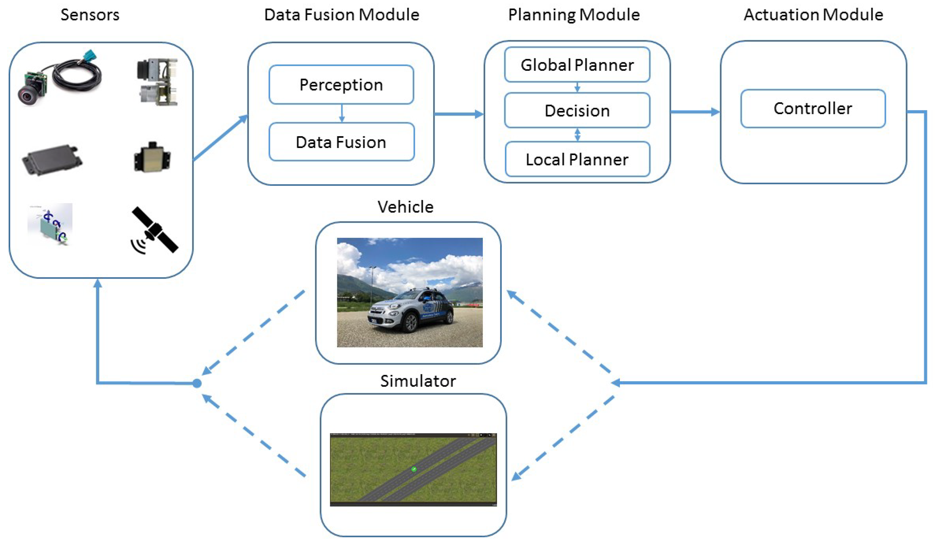
Our System
2. Related Works
3. Sensors, Perception and Data Fusion
3.1. Sensors and Perception
- In the first group, we insert video-cameras. The cameras on the market can produce from 30 to 60 frames per second, and they can easily identify obstacles, relevant traffic signs, and appropriate navigation paths. Common off-the-shelf cameras have low cost, and their output can be manipulated by several applications using computer vision algorithms and/or machine/deep learning approaches [12,37]. Unfortunately, cameras can perform badly in nasty environmental conditions: It is difficult to evaluate distances in rainy conditions, to track lanes in foggy weather, and to discriminate between objects and dark shadows in sunny conditions. For that reasons, using other sensors is in order.
- In the second category, we insert radars. Radars working at a frequency rate from 24 GHz to 76 GHz have a spanning range varying from short to medium, and are thus useless for far-away object detection. Luckily, with the advent of the so-called “long-range radars”, working at 77 GHz, it is now possible to increase ranges up to 200 m and far-away objects do not constitute a problem anymore. Moreover, radars work well in all weather conditions, and the information collected does not degrade with bad weather. Unfortunately, radars have a low resolution, and it is often difficult to discriminate between true and false positive.
- In the third category, we insert LiDARs (Light Detection and Ranging). Lidars are a way for measuring distances by illuminating the target with laser light and evaluating the reflection with a sensor. They produce high-resolution point clouds and quite reliable information thus they deliver good distance estimations and are primarily used for roadside detection (including lane detection), recognition of both static and dynamic objects, Simultaneous Localization and Mapping (SLAM), and 3D environmental map creation. Unfortunately, they may be very expensive. To reduce the cost factor especially on inexpensive cars, Marelli in January 2020 has signed an agreement to develop more practical LiDAR solution for automotive applications, in collaboration with XenomatiX.
- In the fourth category, we insert high precision GPS and IMU (Inertial Measurement Unit) which are needed within the vehicle positioning system. They are fundamental for an autonomous car, because they give the knowledge of the vehicle location.
3.2. Data Fusion
3.3. Data Compression and Memory Optimization
4. The Path-Planner Module
4.1. Global Planner
4.2. Decision-Maker
4.3. Local Planner
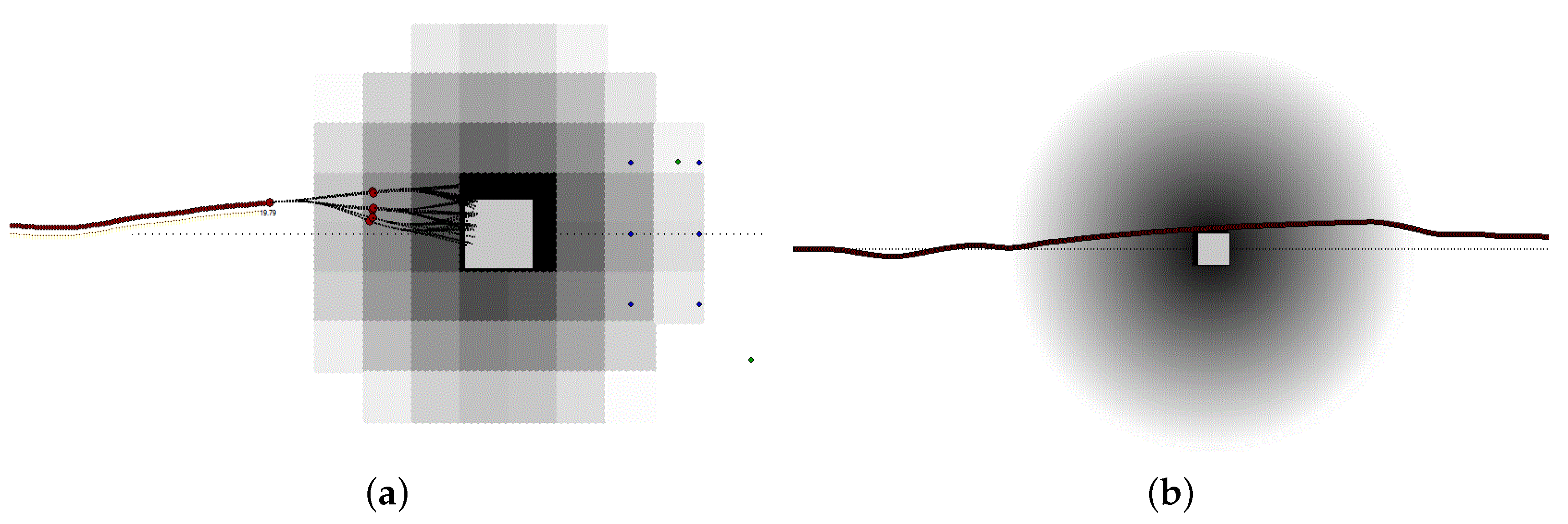
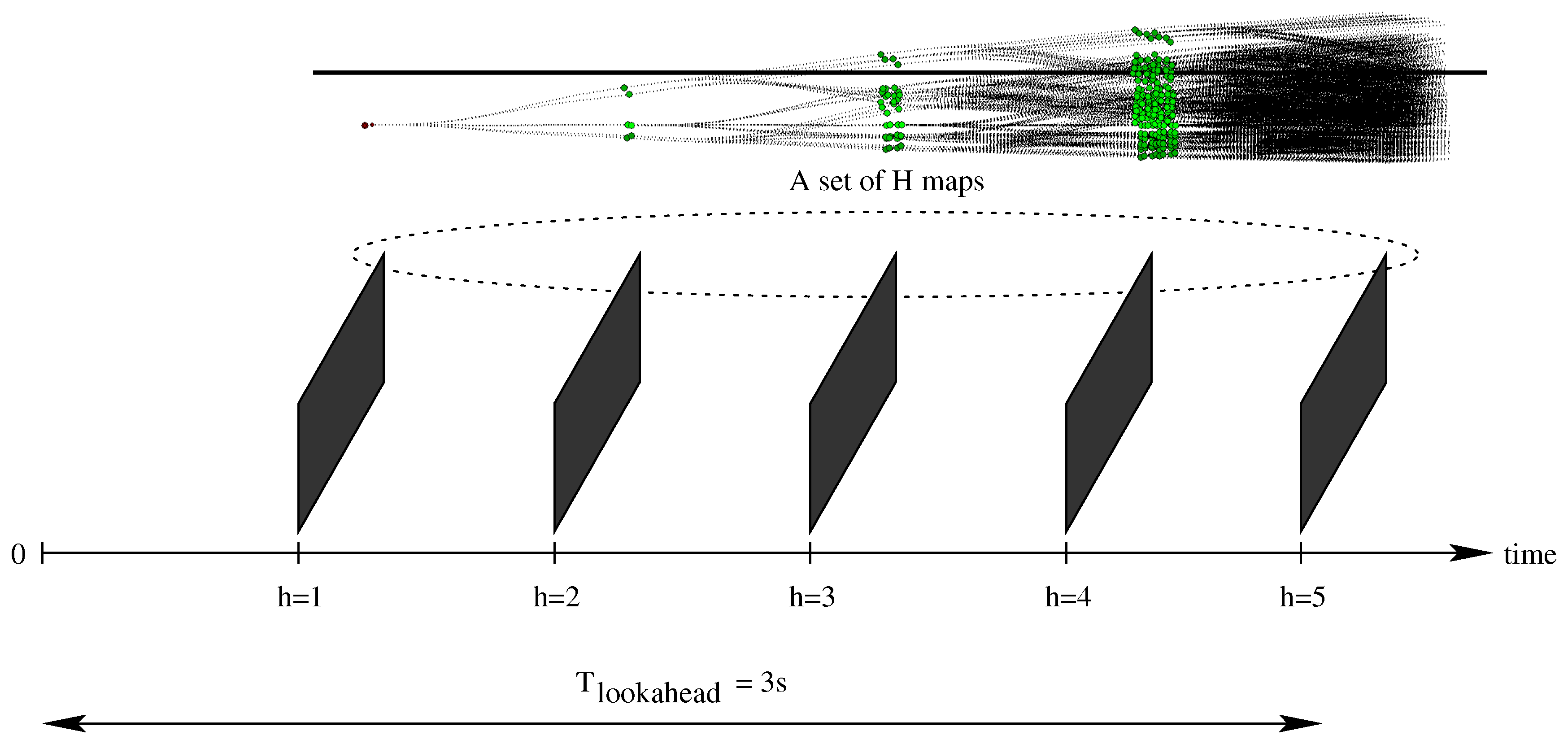
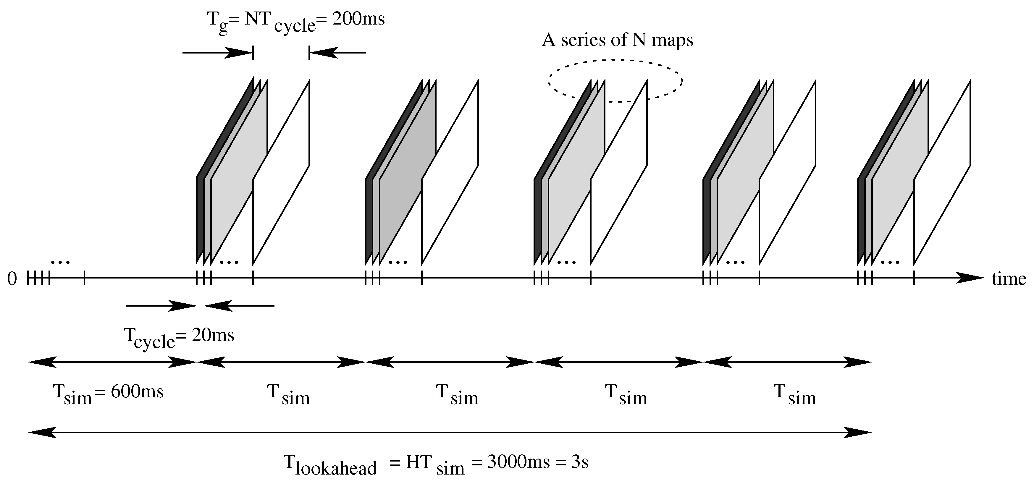
4.4. Expansion Trees and Grid Maps
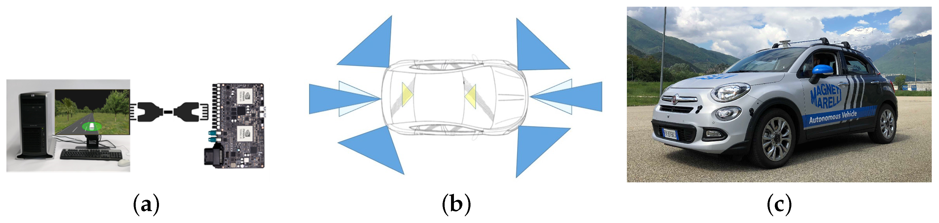
5. Controller and Vehicle Simulator
5.1. Controller
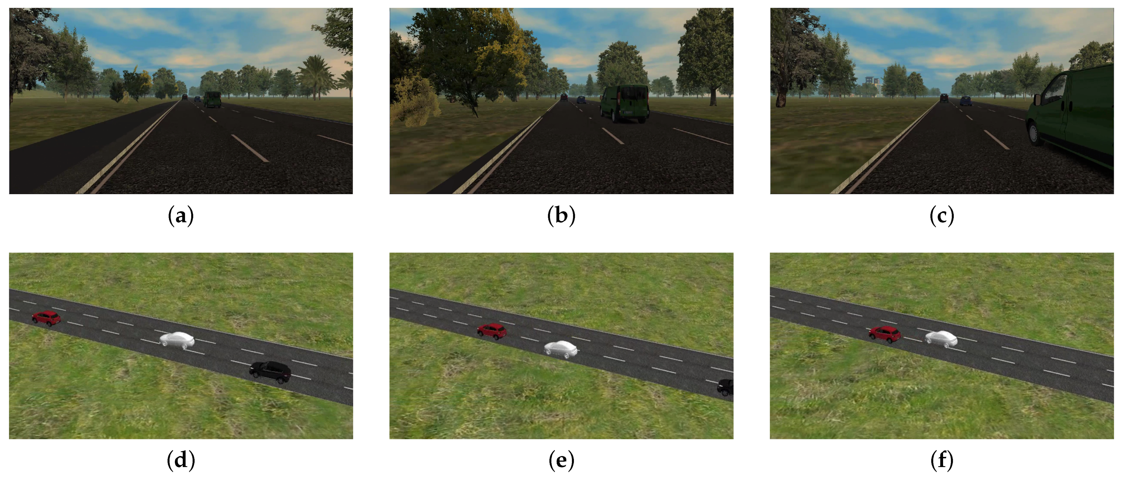
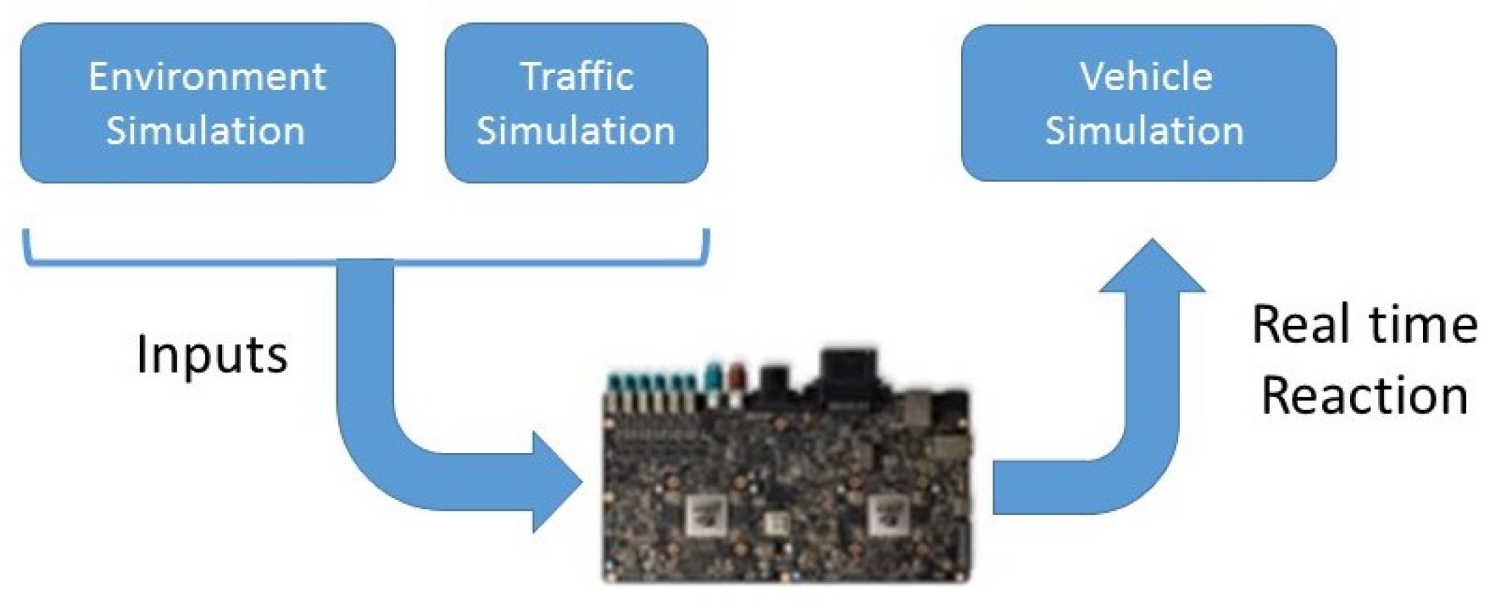
5.2. Vehicle Simulator
- Test the range, accuracy, and tracking capabilities of our environment sensors.
- Check the ability of our fusion system to re-create the environment.
- Verify the trajectory against obstacles and other vehicles.
- Testing the vehicle stability and control accuracy on the control module.
6. Communication Schemes
6.1. Synchronous Path-Planner
6.2. Asynchronous Path Planner
7. Experimental Analysis
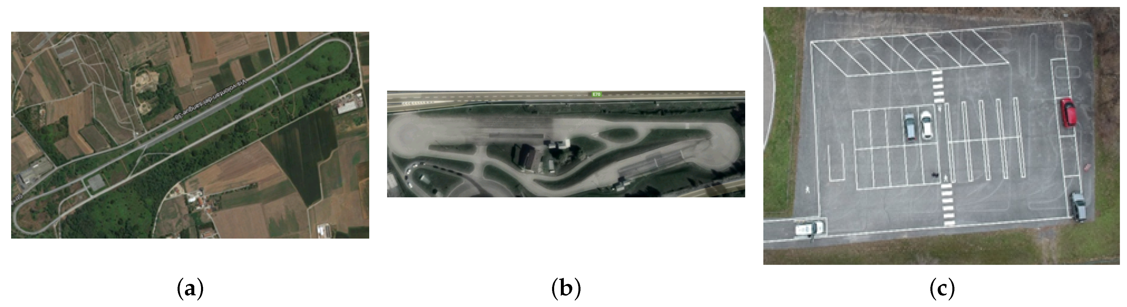
7.1. Experimental Set-Up
- The highway center (Figure 13a) has three lanes, each one with a width included between 3.60 m and 3.75 m and a straight lane longer than 2 Km. As the speed limit is fixed at 130 km/h, this complex enables all scenarios possible on a highway as adaptive cruise control tests, overtaking, entering, exiting, and traffic jam. The standard level of automation in this installation is 3, with a driver on-board at all times.
- The urban facility (please see Figure 13b) has lanes with a width of 2.50 m and a speed limit of 50 km/h. This complex enables typical urban driving conditions as T-intersection, roundabouts, stop and go, traffic jam, and right of way intersections. The minimum level of automation needed in this complex is 3.
- The last installation (reported in Figure 13c) is a parking area facility with the speed limit settled at 15 Km/h. The area includes three different types of parking slots, i.e., parallel, orthogonal, and angular. This kind of scenario is used to test all conditions of a typical valet parking where the vehicle can park itself (level 4 of automation) without any driver or passenger inside.
- A CPU Intel Core i7-6700 HQ with 2.60 GHz and 8.00 GByte of RAM memory.
- A PX2 NVIDIA pascal GPU PG418 up to 3 GHz and 8.00 GByte DRAM per Parker.
7.2. Validation Methods
- The mean squared error (MSE) measures the average of the squares of the errors:It is the second moment (about the origin) of the error and thus incorporates the variance of the calibration curve:
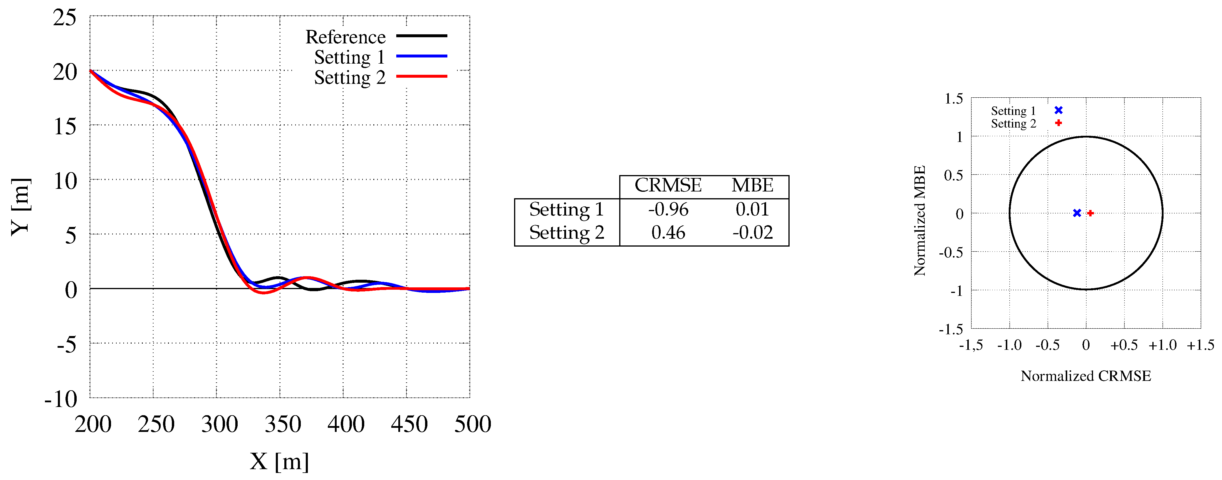
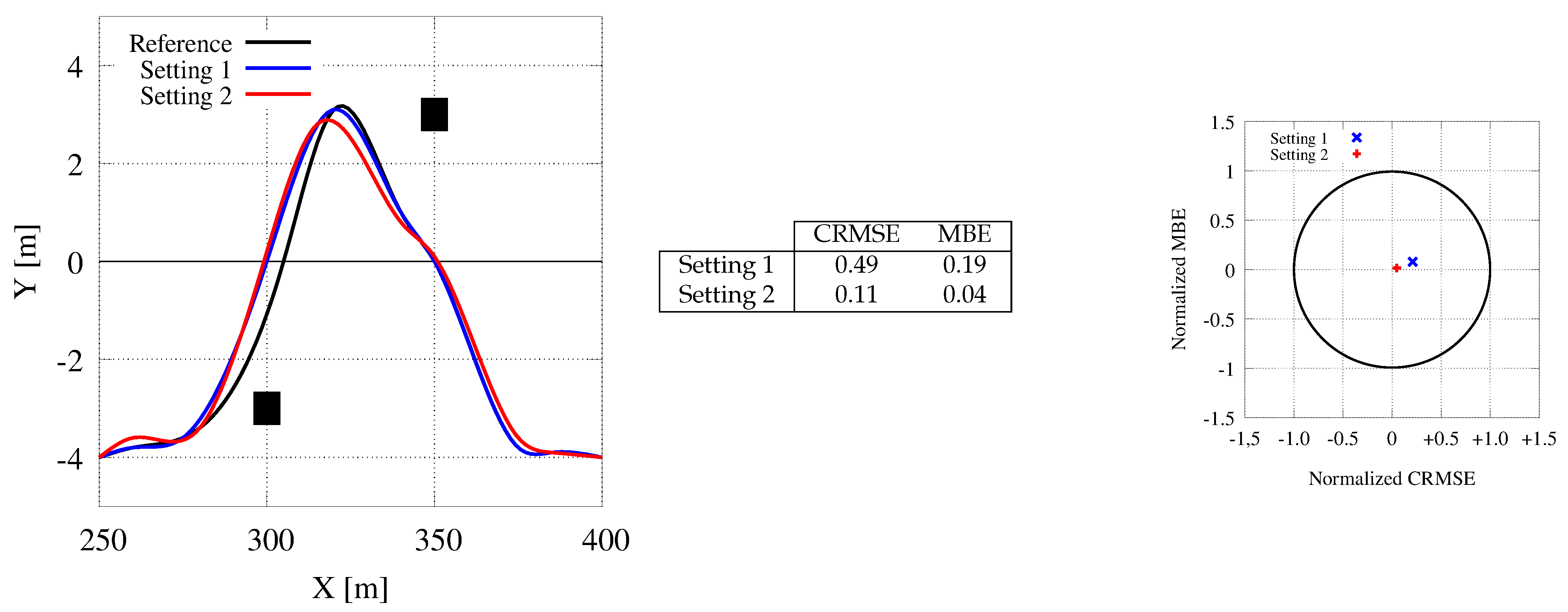
- The Mean Bias Error (MBE) is usually adopted to capture the average bias in a prediction and it is defined as follow:
- The root mean squared error (RMSE) compares data sets with different sizes, since it is measured on the same scale as the target value. It is obtained as the square root of the MSE, i.e.,RMSE essentially measures the root of the mean square distance between the computed trajectory and the desired one. Usually, RMSE as to be as small as possible.
- The Centered Root Mean Square Error (CRMSE) is the RMSE corrected for bias. The CRMSE is defined as:where is the standard deviation of the measure.
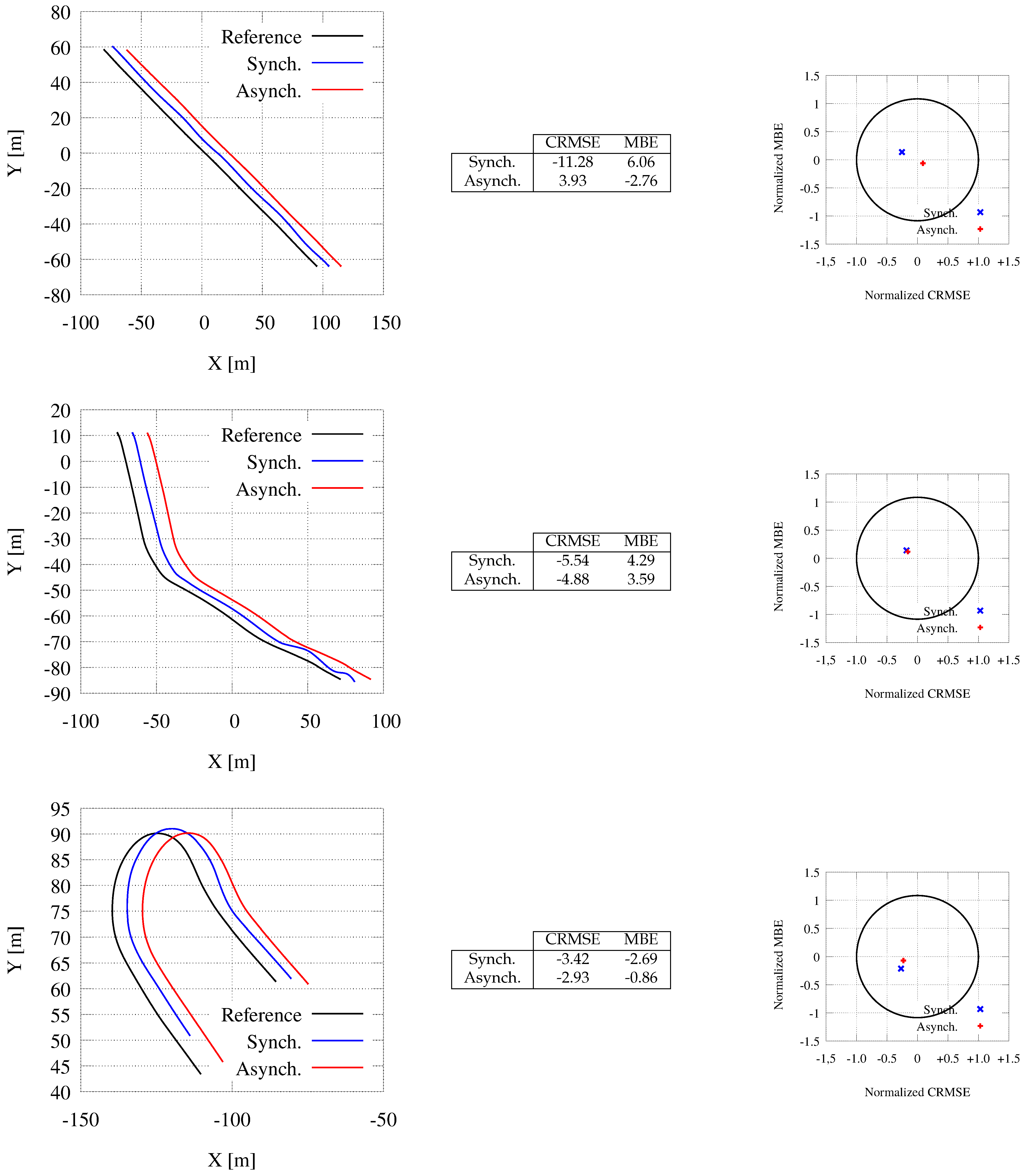
7.3. Comparing the Synchronous and the Asynchronous Mode
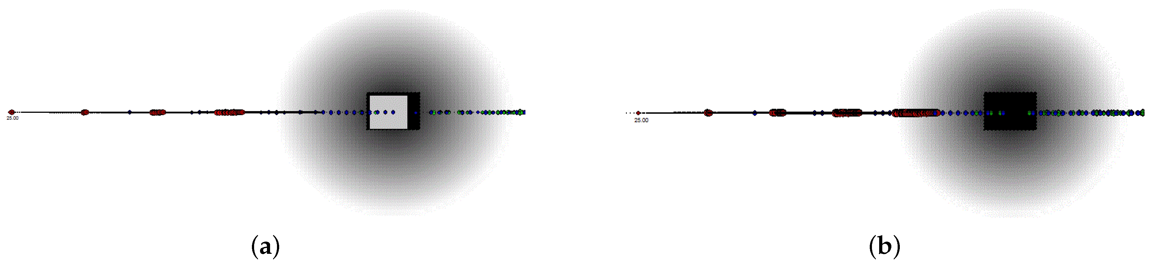
7.4. Obstacle Avoidance
- Reduced the grid-map resolution to pixels and we displaced the car such that the map in front of the vehicle represents a larger area than the one spanned behind it.
- Represented the probability of each location of each grid map with a reduced accuracy, i.e., using a short integer for each location.
- Merged all maps within the same map series into the same grid map.
- Used textures memory to represent from 4 to 16 different grid maps eventually belonging to the same series of maps or to the same set of maps.
- Used the same grid map computed for the tree level , for each further computation level with .
7.5. Back on Track
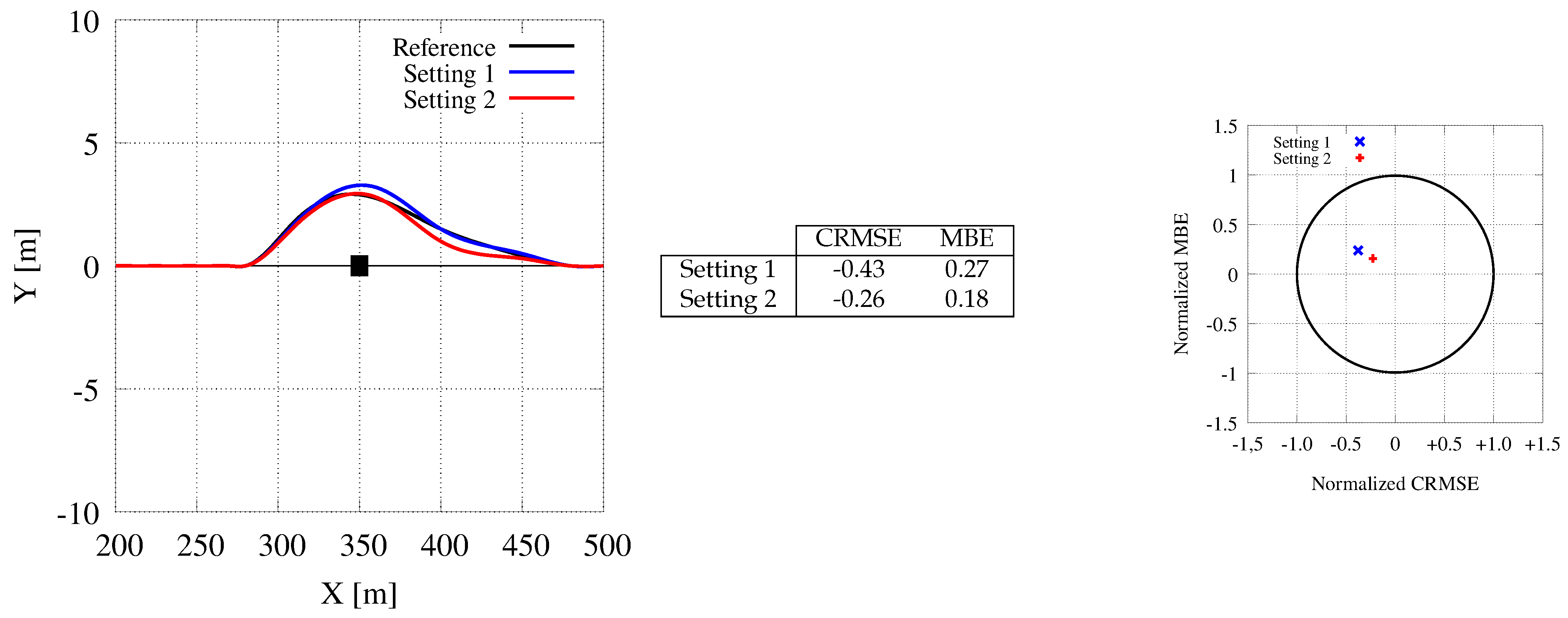
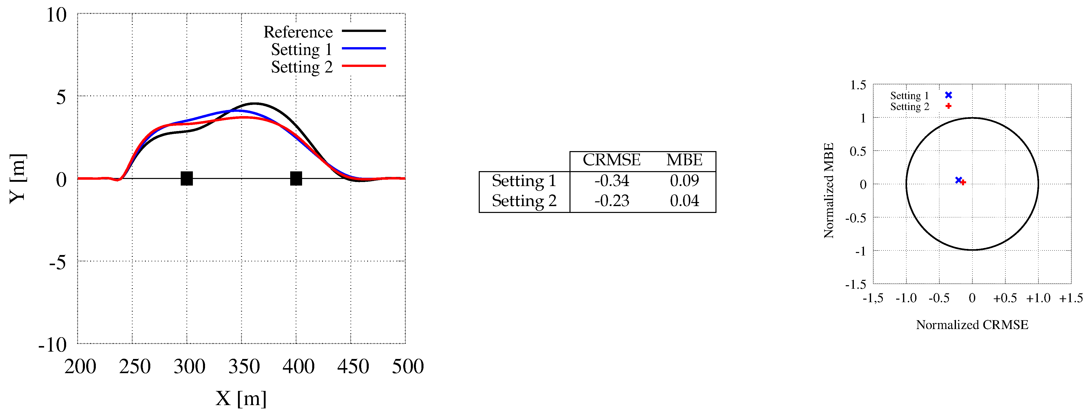
7.6. The Moose or elk Test
8. Conclusions
Author Contributions
Funding
Conflicts of Interest
References
- Singh, S. Critical Reasons for Crashes Investigated in the National Motor Vehicle Crash Causation Survey; Report No. DOT HS 812 115; National Highway Traffic Safety Administration: Washington, DC, USA, 2015.
- Singh, S. Critical Reasons for Crashes Investigated in the National Motor Vehicle Crash Causation Survey; Report No. DOT HS 812 506; National Highway Traffic Safety Administration: Washington, DC, USA, 2018.
- Blanco, M.; Atwood, J.; Russell, S.M.; Trimble, T.; McClafferty, J.A.; Perez, M.A. Automated Vehicle Crash Rate Comparison Using Naturalistic Data; Technical Report; Virginia Tech Transportation Institute: Blacksburg, VA, USA, 2016. [Google Scholar] [CrossRef]
- Kalra, N.; Paddock, S. Driving to Safety: How Many Miles of Driving Would it Take to Demonstrate Autonomous Vehicle Reliability? Transp. Res. Part Policy Pract. 2016, 94, 182–193. [Google Scholar] [CrossRef]
- SAE International. Taxonomy and Definitions for Terms Related to Driving Automation Systems for On-Road Motor Vehicles (International standard J3016_201609). 2016. Available online: https://www.sae.org/standards/content/j3016_201609/ (accessed on 1 December 2020). [CrossRef]
- Schwesinger, U.; Rufli, M.; Furgale, P.; Siegwart, R. A sampling-based partial motion planning framework for system-compliant navigation along a reference path. In Proceedings of the 2013 IEEE Intelligent Vehicles Symposium (IV), Gold Coast, QLD, Australia, 23–26 June 2013; pp. 391–396. [Google Scholar] [CrossRef]
- Cabodi, G.; Camurati, P.; Garbo, A.; Giorelli, M.; Quer, S.; Savarese, F. A Smart Many-Core Implementation of a Motion Planning Framework along a Reference Path for Autonomous Cars. Electronics 2019, 8, 177. [Google Scholar] [CrossRef]
- Buehler, M.; Iagnemma, K.; Singh, S. The 2005 DARPA Grand Challenge: The Great Robot Race, 1st ed.; Springer Publishing Company: Berlin/Heidelberg, Germany, 2007. [Google Scholar]
- Buehler, M.; Iagnemma, K.; Singh, S. The DARPA Urban Challenge: Autonomous Vehicles in City Traffic, 1st ed.; Springer Publishing Company: Berlin/Heidelberg, Germany, 2009. [Google Scholar]
- Huang, Y.; Chen, Y. Survey of State-of-Art Autonomous Driving Technologies with Deep Learning. In Proceedings of the IEEE 20th International Conference on Software Quality, Reliability and Security Companion (QRS-C), Macau, China, 11–14 December 2020; pp. 221–228. [Google Scholar] [CrossRef]
- Yurtsever, E.; Lambert, J.; Carballo, A.; Takeda, K. A Survey of Autonomous Driving: Common Practices and Emerging Technologies. IEEE Access 2020, 8, 58443–58469. [Google Scholar] [CrossRef]
- Grigorescu, S.; Trasnea, B.; Cocias, T.; Macesanu, G. A Survey of Deep Learning Techniques for Autonomous Driving. J. Field Robot. 2020, 37, 362–386. [Google Scholar] [CrossRef]
- Valiska, J.; Marchevský, S.; Kokoska, R. Object Tracking by Color-based Particle Filter Techniques in Videosequences. In Proceedings of the 24th International Conference Radioelektronika, Bratislava, Slovakia, 15–16 April 2014; pp. 1–4. [Google Scholar] [CrossRef]
- Yildirim, M.E.; Song, J.; Park, J.; Yoon, B.; Yu, Y. Robust Vehicle Tracking Multi-feature Particle Filter. In International Conference on Multimedia, Computer Graphics, and Broadcasting; Springer: Berlin/Heidelberg, Germany, 2011; Volume 263, pp. 191–196. [Google Scholar] [CrossRef]
- Qing, M.; Jo, K.H. A Novel Particle Filter Implementation for a Multiple-Vehicle Detection and Tracking System Using Tail Light Segmentation. Int. J. Control. Autom. Syst. 2013, 11, 577–585. [Google Scholar] [CrossRef]
- Chan, Y.M.; Huang, S.S.; Fu, L.C.; Hsiao, P.Y.; Lo, M.F. Vehicle Detection and Tracking Under Various Lighting Conditions Using a Particle Filter. Intell. Transp. Syst. 2012, 6, 1–8. [Google Scholar] [CrossRef]
- Zhao, Z.; Zheng, P.; Xu, S.; Wu, X. Object Detection with Deep Learning: A Review. IEEE Trans. Neural Networks Learn. Syst. 2019, 30, 3212–3232. [Google Scholar] [CrossRef] [PubMed]
- Xiongwei, W.; Sahoo, D.; Hoi, S. Recent Advances in Deep Learning for Object Detection. Neurocomputing 2020, 396, 39–64. [Google Scholar] [CrossRef]
- Girshick, R.; Donahue, J.; Darrell, T.; Malik, J. Rich Feature Hierarchies for Accurate Object Detection and Semantic Segmentation. In Proceedings of the IEEE Conference on Computer Vision and Pattern Recognition, Columbus, OH, USA, 23–28 June 2014; pp. 580–587. [Google Scholar] [CrossRef]
- Redmon, J.; Divvala, S.K.; Girshick, R.B.; Farhadi, A. You Only Look Once: Unified, Real-Time Object Detection. In Proceedings of the IEEE Conference on Computer Vision and Pattern Recognition (CVPR), Boston, MA, USA, 7–12 June 2015. [Google Scholar]
- Petrovska, B.; Atanasova-Pacemska, T.; Corizzo, R.; Mignone, P.; Lameski, P.; Zdravevski, E. Aerial Scene Classification through Fine-Tuning with Adaptive Learning Rates and Label Smoothing. Appl. Sci. 2020, 10, 5792. [Google Scholar] [CrossRef]
- Matthaei, R.; Lichte, B.; Maurer, M. Robust Grid-Based Road Detection for ADAS and Autonomous Vehicles in Urban Environments. In Proceedings of the 16th International Conference on Information Fusion, Istanbul, Turkey, 9–12 July 2013; pp. 938–944. [Google Scholar]
- Kretzschmar, H.; Stachniss, C. Information-Theoretic Compression of Pose Graphs for Laser-based SLAM. Int. J. Robot. Res. 2012, 31, 1219–1230. [Google Scholar] [CrossRef]
- Kretzschmar, H.; Stachniss, C. Pose Graph Compression for Laser-Based SLAM; Springer Tracts in Advanced Robotics: Cham, Switzerland, 2016. [Google Scholar]
- Solea, R.; Nunes, U. Trajectory Planning with Velocity Planner for Fully-Automated Passenger Vehicles. In Proceedings of the 2006 IEEE Intelligent Transportation Systems Conference, Toronto, ON, Canada, 17–20 September 2006; pp. 474–480. [Google Scholar] [CrossRef]
- Werling, M.; Kammel, S.; Ziegler, J.; Gröll, L. Optimal Trajectories for Time-Critical Street Scenarios Using Discretized Terminal Manifolds. Int. J. Robot. Res. 2012, 31, 346–359. [Google Scholar] [CrossRef]
- Ma, L.; Xue, J.; Kawabata, K.; Zhu, J.; Ma, C.; Zheng, N. Efficient Sampling-Based Motion Planning for On-Road Autonomous Driving. IEEE Trans. Intell. Transp. Syst. 2015, 16, 1961–1976. [Google Scholar] [CrossRef]
- LaValle, S.M.; Kuffner, J.J. Randomized Kinodynamic Planning. Int. J. Robot. Res. 2001, 20, 378–400. [Google Scholar] [CrossRef]
- Pan, J.; Lauterbach, C.; Manocha, D. g-Planner: Real-time Motion Planning and Global Navigation Using GPUs. In Proceedings of the Twenty-Fourth AAAI Conference on Artificial Intelligence, Atlanta, GA, USA, 11–15 July 2010; pp. 1245–1251. [Google Scholar]
- Kider, J.T.; Henderson, M.; Likhachev, M.; Safonova, A. High-Dimensional Planning on the GPU. In Proceedings of the 2010 IEEE International Conference on Robotics and Automation, Anchorage, AK, USA, 3–7 May 2010; pp. 2515–2522. [Google Scholar]
- McNaughton, M.; Urmson, C.; Dolan, J.M.; Lee, J.W. Motion Planning for Autonomous Driving with a Conformal Spatiotemporal Lattice. In Proceedings of the 2011 IEEE International Conference on Robotics and Automation, Shanghai, China, 9–13 May 2011. [Google Scholar]
- Heinrich, S.; Zoufahl, A.; Rojas, R. Real-time Trajectory Optimization Under Motion Uncertainty Using a GPU. In Proceedings of the 2015 IEEE/RSJ International Conference on Intelligent Robots and Systems (IROS), Hamburg, Germany, 28 September–2 October 2015; pp. 3572–3577. [Google Scholar] [CrossRef]
- Huang, W.; Wang, K.; Lv, Y.; Zhu, F. Autonomous Vehicles Testing Methods Review. In Proceedings of the 2016 IEEE 19th International Conference on Intelligent Transportation Systems (ITSC), Rio de Janeiro, Brazil, 1–4 November 2016; pp. 163–168. [Google Scholar]
- Chen, Y.; Chen, S.; Zhang, T.; Zhang, S.; Zheng, N. Autonomous Vehicle Testing and Validation Platform: Integrated Simulation System with Hardware in the Loop. In Proceedings of the 2018 IEEE Intelligent Vehicles Symposium (IV), Changshu, China, 26–30 June 2018; pp. 949–956. [Google Scholar]
- Kocić, J.; Jovičić, N.; Drndarević, V. Sensors and Sensor Fusion in Autonomous Vehicles. In Proceedings of the 26th Telecommunications Forum (TELFOR), Belgrade, Serbia, 20–21 November 2018; pp. 420–425. [Google Scholar] [CrossRef]
- Kang, I.; Cimurs, R.; Lee, J.H.; Hong Suh, I. Fusion Drive: End-to-End Multi Modal Sensor Fusion for Guided Low-Cost Autonomous Vehicle. In Proceedings of the 17th International Conference on Ubiquitous Robots (UR), Kyoto, Japan, 22–26 June 2020; pp. 421–428. [Google Scholar] [CrossRef]
- Cheng, C.; Gulati, D.; Yan, R. Architecting Dependable Learning-enabled Autonomous Systems: A Survey. arXiv 2019, arXiv:1902.10590. [Google Scholar]
- Open Autonomous Driving. Positioning Sensors for Autonoumous Vehicles. Available online: https://autonomous-driving.org/2019/01/25/positioning-sensors-for-autonomous-vehicles/ (accessed on 20 April 2020).
- Thrun, S.; Bücken, A. Integrating Grid-based and Topological Maps for Mobile Robot Navigation. In Proceedings of the Thirteenth National Conference on Artificial Intelligence—Volume 2, Portland, OR, USA, 4–8 August 1996; pp. 944–950. [Google Scholar]
- Li, M.; Feng, Z.; Stolz, M.; Kunert, M.; Henze, R.; Küçükay, F. High Resolution Radar-based Occupancy Grid Mapping and Free Space Detection. In Proceedings of the 4th International Conference on Vehicle Technology and Intelligent Transport Systems, Funchal, Portugal, 16–18 March 2018; pp. 70–81. [Google Scholar] [CrossRef]
- Doggett, M.C. Texture Caches. IEEE Micro 2012, 32, 136–141. [Google Scholar] [CrossRef]
- Rodríguez-Canosa, G.; Thomas, S.; Cerro, J.; Barrientos, A.; Macdonald, B. A Real-Time Method to Detect and Track Moving Objects (DATMO) from Unmanned Aerial Vehicles (UAVs) Using a Single Camera. Remote Sens. 2012, 4, 1090–1111. [Google Scholar] [CrossRef]
- Royden, C.; Sannicandro, S.; Webber, L. Detection of Moving Objects Using Motion- and Stereo-tuned Operators. J. Vis. 2015, 15, 21. [Google Scholar] [CrossRef] [PubMed][Green Version]
- You, C.; Lu, J.; Filev, D.; Tsiotras, P. Highway Traffic Modeling and Decision Making for Autonomous Vehicle Using Reinforcement Learning. In Proceedings of the 2018 IEEE Intelligent Vehicles Symposium (IV), Changshu, China, 26–30 June 2018. [Google Scholar] [CrossRef]
- Marín, P.; Hussein, A.; Martín Gómez, D.; de la Escalera, A. Global and Local Path Planning Study in a ROS-Based Research Platform for Autonomous Vehicles. J. Adv. Transp. 2018, 2018, 1–10. [Google Scholar] [CrossRef]
- Hegedüs, F.; Bécsi, T.; Aradi, S.; Gáldi, G. Hybrid Trajectory Planning for Autonomous Vehicles using Neural Networks. In Proceedings of the 2018 IEEE 18th International Symposium on Computational Intelligence and Informatics (CINTI), Budapest, Hungary, 21–22 November 2018; pp. 25–30. [Google Scholar]
- Mirchevska, B.; Pek, C.; Werling, M.; Althoff, M.; Boedecker, J. High-level Decision Making for Safe and Reasonable Autonomous Lane Changing using Reinforcement Learning. In Proceedings of the 2018 21st International Conference on Intelligent Transportation Systems (ITSC), Maui, HI, USA, 4–7 November 2018. [Google Scholar] [CrossRef]
- Hubmann, C.; Becker, M.; Althoff, D.; Lenz, D.; Stiller, C. Decision Making for Autonomous Driving Considering Interaction and Uncertain Prediction of Surrounding Vehicles. In Proceedings of the 2017 IEEE Intelligent Vehicles Symposium (IV), Los Angeles, CA, USA, 11–14 June 2017; pp. 1671–1678. [Google Scholar] [CrossRef]
- Alonso, L.; Pérez-Oria, J.; Al-Hadithi, B.; Jiménez, A. Self-Tuning PID Controller for Autonomous Car Tracking in Urban Traffic. In Proceedings of the 2013 17th International Conference on System Theory, Control and Computing (ICSTCC), Sinaia, Romania, 11–13 October 2013. [Google Scholar] [CrossRef]
- Lin, Y.C.; Hsu, H.C.; Chen, W.J. Dynamic Programming for Model Predictive Control of Adaptive Cruise Control Systems. In Proceedings of the 2015 IEEE International Conference on Vehicular Electronics and Safety (ICVES), Yokohama, Japan, 5–7 November 2015; pp. 202–207. [Google Scholar] [CrossRef]
- Trotta, A.; Cirillo, A.; Giorelli, M. A Feedback Linearization Based Approach for Fully Autonomous Adaptive Cruise Control. In Proceedings of the 2019 18th European Control Conference (ECC), Naples, Italy, 25–28 June 2019. [Google Scholar] [CrossRef]
- Raffin, A.; Taragna, M.; Giorelli, M. Adaptive Longitudinal Control of an Autonomous Vehicle with an Approximate Knowledge of its Parameters. In Proceedings of the 2017 11th International Workshop on Robot Motion and Control (RoMoCo), Wasowo, Poland, 3–5 July 2017; pp. 1–6. [Google Scholar] [CrossRef]
- Dixit, V.; Xu, Z.; Wang, M.; Zhang, F.; Jin, S.; Zhang, J.; Zhao, X. PaTAVTT: A Hardware-in-the-Loop Scaled Platform for Testing Autonomous Vehicle Trajectory Tracking. J. Adv. Transp. 2017, 2017, 9203251. [Google Scholar]
- Jolliff, J.; Kindle, J.; Shulman, I.; Penta, B.; Friedrichs, M.; Helber, R.; Arnone, R. Summary Diagrams for Coupled Hydrodynamic-Ecosystem Model Skill Assessment. J. Mar. Syst. 2009, 76, 64–82. [Google Scholar] [CrossRef]


| Vehicle Characteristics | Values |
|---|---|
| Width | 2 m |
| Maximum lateral offset | 0.8 m |
| Speed | [13 m/s, 36 m/s] |
| [46.8 Km/h, 29.6 Km/h] | |
| Acceleration (standard) | [−2 m/s, +2 m/s] |
| Acceleration (emergency) | [−9.81 m/s, +9.81 m/s] |
Publisher’s Note: MDPI stays neutral with regard to jurisdictional claims in published maps and institutional affiliations. |
© 2021 by the authors. Licensee MDPI, Basel, Switzerland. This article is an open access article distributed under the terms and conditions of the Creative Commons Attribution (CC BY) license (http://creativecommons.org/licenses/by/4.0/).
Share and Cite
Quer, S.; Garcia, L. Modules and Techniques for Motion Planning: An Industrial Perspective. Sensors 2021, 21, 420. https://doi.org/10.3390/s21020420
Quer S, Garcia L. Modules and Techniques for Motion Planning: An Industrial Perspective. Sensors. 2021; 21(2):420. https://doi.org/10.3390/s21020420
Chicago/Turabian StyleQuer, Stefano, and Luz Garcia. 2021. "Modules and Techniques for Motion Planning: An Industrial Perspective" Sensors 21, no. 2: 420. https://doi.org/10.3390/s21020420
APA StyleQuer, S., & Garcia, L. (2021). Modules and Techniques for Motion Planning: An Industrial Perspective. Sensors, 21(2), 420. https://doi.org/10.3390/s21020420