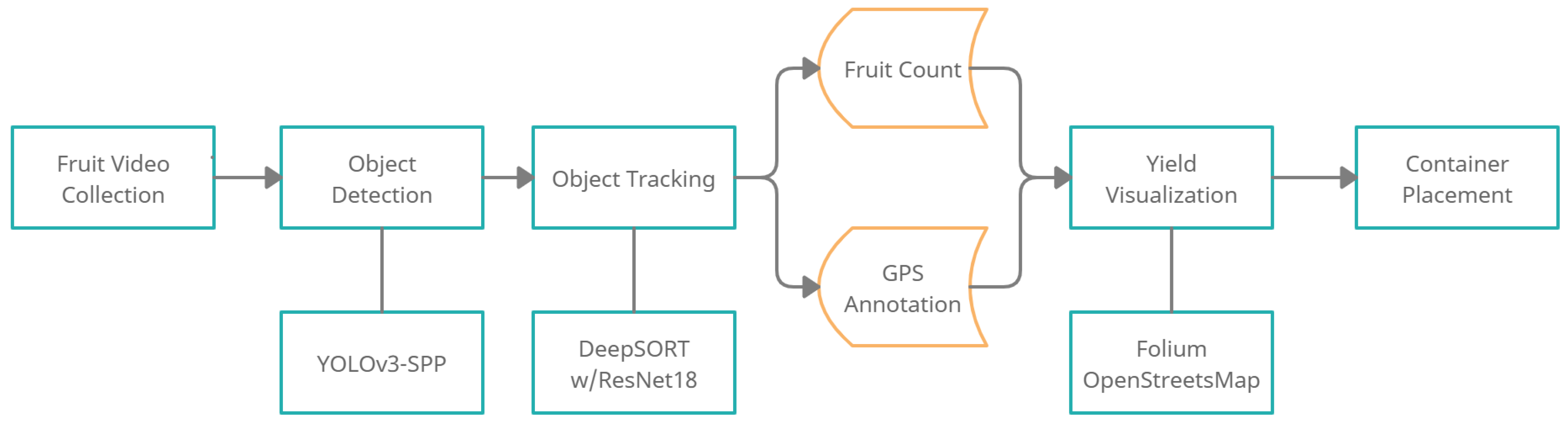
Figure 1.
An end-to-end overview of the proposed smart harvesting pipeline.
Figure 1.
An end-to-end overview of the proposed smart harvesting pipeline.
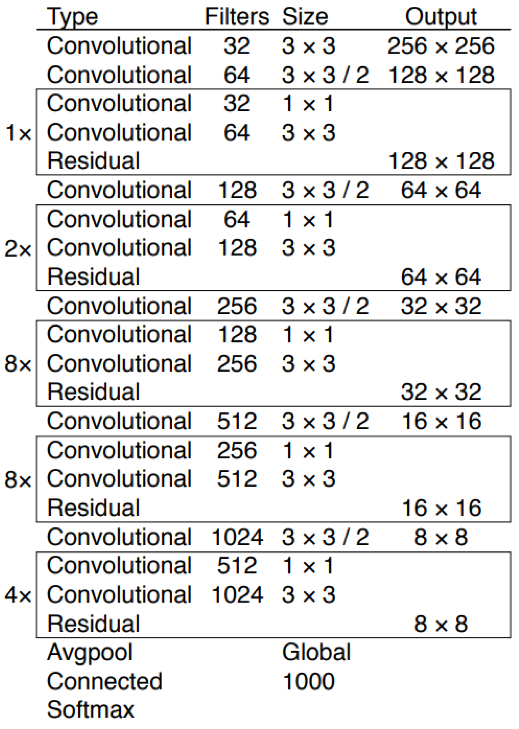
Figure 2.
Darknet53 architecture that is used as YOLOv3’s backbone [
19].
Figure 2.
Darknet53 architecture that is used as YOLOv3’s backbone [
19].
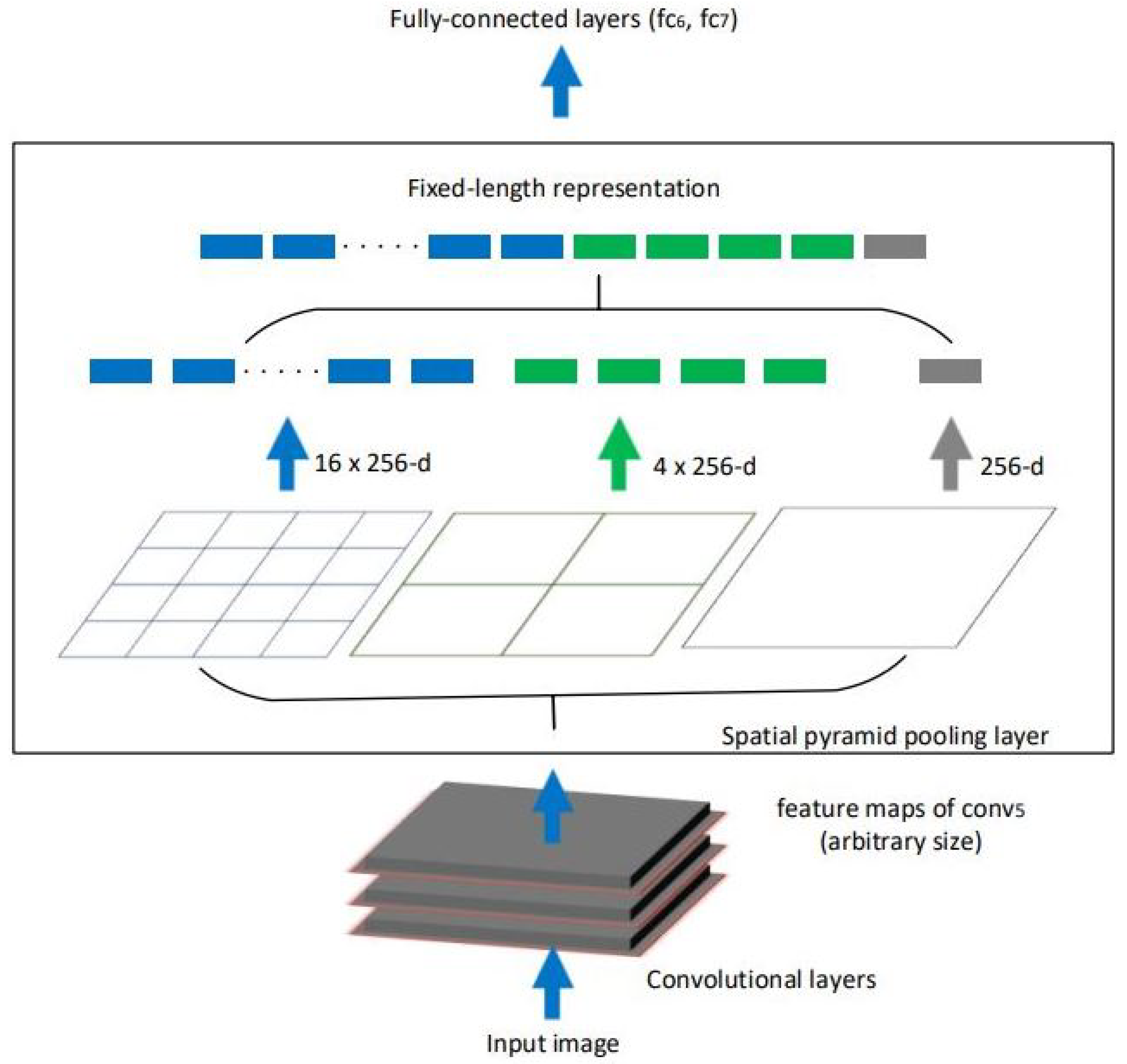
Figure 3.
Visualization of SPP, reproduced from [
23].
Figure 3.
Visualization of SPP, reproduced from [
23].
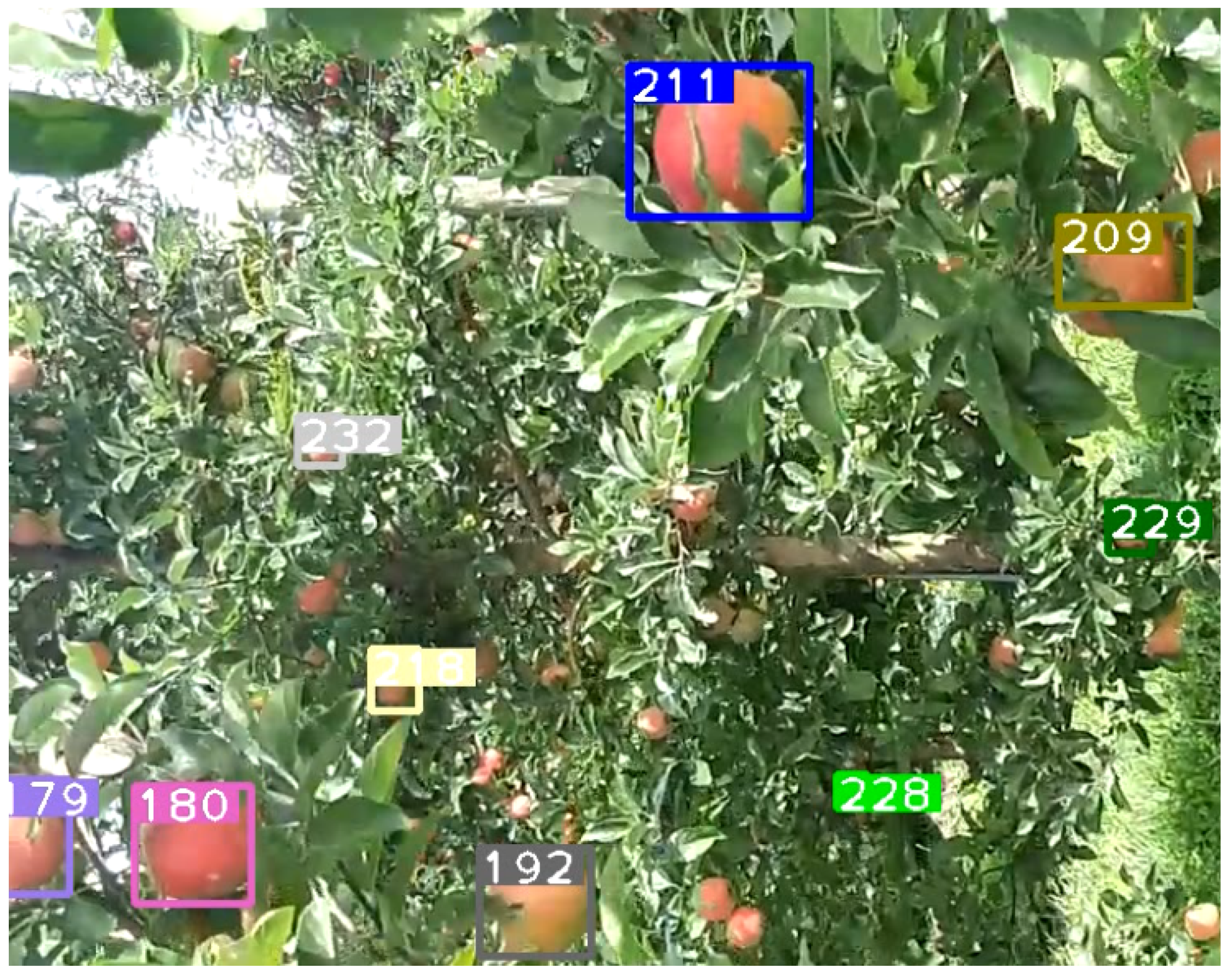
Figure 4.
From the apple orchard video used, some apples from a back row tree are being detected and tracked.
Figure 4.
From the apple orchard video used, some apples from a back row tree are being detected and tracked.
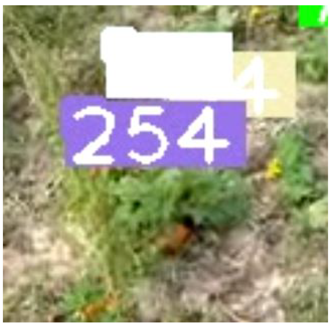
Figure 5.
First apple detected in first frame and is inserted into the tracker which identifies it as track 1.
Figure 5.
First apple detected in first frame and is inserted into the tracker which identifies it as track 1.
Figure 6.
Apple identified in second the frame, noted as detection 1 is tested for association.
Figure 6.
Apple identified in second the frame, noted as detection 1 is tested for association.
Figure 7.
Second apple identified in the second frame, noted as detection 2 is tested for association.
Figure 7.
Second apple identified in the second frame, noted as detection 2 is tested for association.
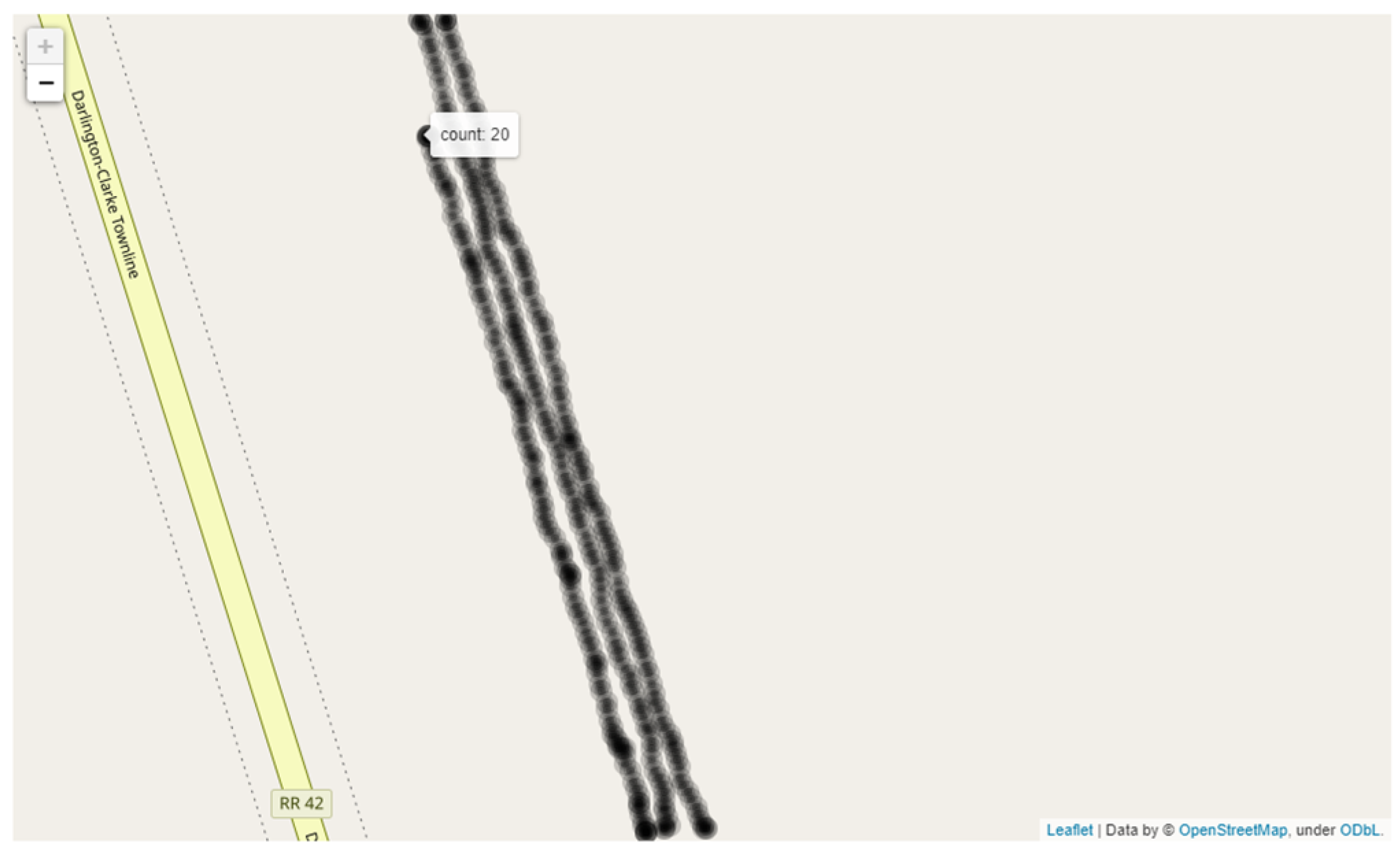
Figure 8.
Mapping the GPS data after counting.
Figure 8.
Mapping the GPS data after counting.
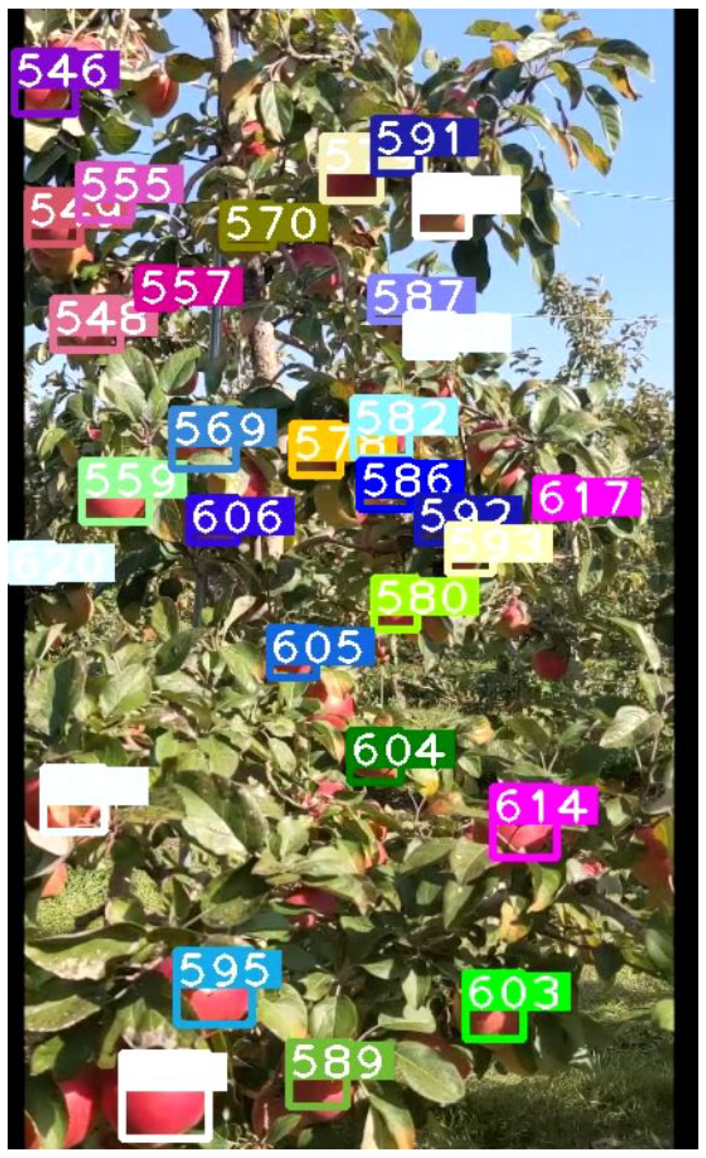
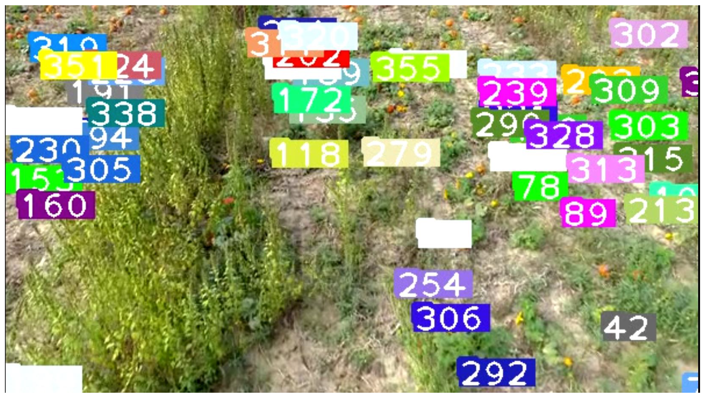
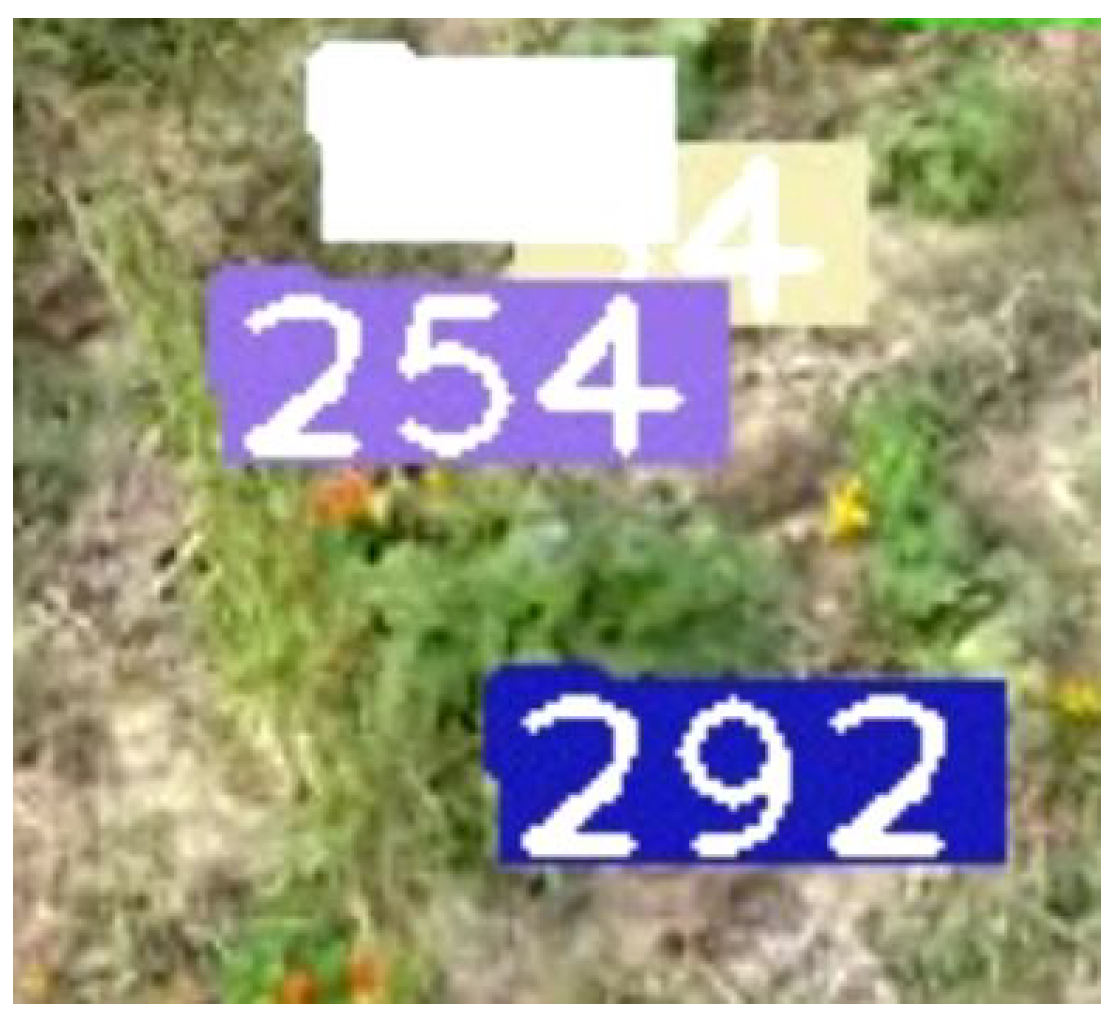
Figure 9.
A frame taken from the video of the apple tree during runtime, just in this frame there are approximately 30 apples being tracked, in addition to the saved tracks that are not currently detected. There are several apples that are largely occluded for which one of the following scenarios could be true: (1) previously detected and counted before becoming obscured; (2) will be detected next with the camera motion or with a clearer angle; (3) will fail to be detected leading to a loss in counting accuracy.
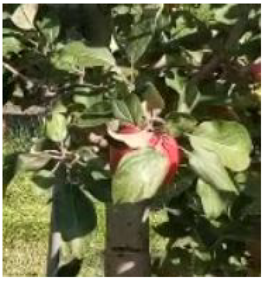
Figure 10.
The leaf covers the apple and is predominantly visible. We avoid annotating such apples to avoid mistakenly detecting leaves as apples and will instead rely on the angle eventually making the apple clearer.
Figure 10.
The leaf covers the apple and is predominantly visible. We avoid annotating such apples to avoid mistakenly detecting leaves as apples and will instead rely on the angle eventually making the apple clearer.
Figure 11.
The apple does indeed become clearer in the following frame, allowing for detection to occur and the tracker to save and count the apple.
Figure 11.
The apple does indeed become clearer in the following frame, allowing for detection to occur and the tracker to save and count the apple.
Figure 12.
A frame taken from the video showing the view of the pumpkins and all of the current detections, the numbers denote the track ID.
Figure 12.
A frame taken from the video showing the view of the pumpkins and all of the current detections, the numbers denote the track ID.
Figure 13.
Another pumpkin that is hidden and is not currently detected nor counted.
Figure 13.
Another pumpkin that is hidden and is not currently detected nor counted.
Figure 14.
The change in view as the drone flies forward allows more of the pumpkin to be seen, thus is successfully detected and given a track ID.
Figure 14.
The change in view as the drone flies forward allows more of the pumpkin to be seen, thus is successfully detected and given a track ID.
Figure 15.
Pumpkin is mostly hidden and is hard to be seen due to little to no lighting, in further frames the pumpkin only becomes more hidden and is never detected.
Figure 15.
Pumpkin is mostly hidden and is hard to be seen due to little to no lighting, in further frames the pumpkin only becomes more hidden and is never detected.
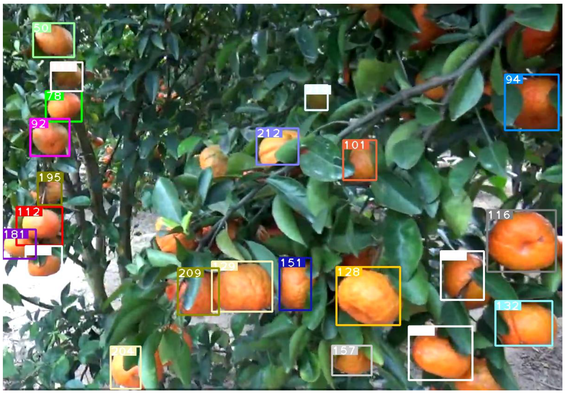
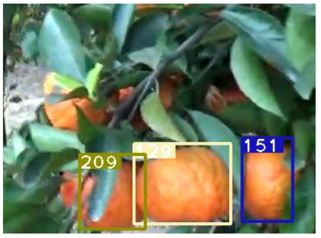
Figure 16.
A view of detected oranges in the tree, numbers denote track ID.
Figure 16.
A view of detected oranges in the tree, numbers denote track ID.
Figure 17.
The majority of uncounted oranges are heavily obscured behind other oranges and leaves, the YOLO pretrained weights don’t fully accommodate brightness and occlusion challenges.
Figure 17.
The majority of uncounted oranges are heavily obscured behind other oranges and leaves, the YOLO pretrained weights don’t fully accommodate brightness and occlusion challenges.
Figure 18.
The container placements visualized using Folium and OpenStreetsMap template. The distance between the containers is evenly spaced across the row, ensuring harvesters will have a container near them.
Figure 18.
The container placements visualized using Folium and OpenStreetsMap template. The distance between the containers is evenly spaced across the row, ensuring harvesters will have a container near them.
Figure 19.
The distance between the containers is uneven, with the last two containers being close to one another. This means that harvesters between the 2nd and 3rd boxes will walk longer distances. There might also be a crowd around the 3rd and 4th boxes as they are fairly close to one another.
Figure 19.
The distance between the containers is uneven, with the last two containers being close to one another. This means that harvesters between the 2nd and 3rd boxes will walk longer distances. There might also be a crowd around the 3rd and 4th boxes as they are fairly close to one another.
Table 1.
Comparison between different SSD models.
Table 1.
Comparison between different SSD models.
| Method | Backbone | AP | FPS (Batch Size of 1) | GPU |
|---|
| YOLOv3-512 [19] | Darknet-53 [19,30] | | 48.7 | Telsa P100 (10 TFLOPS) |
| YOLOv3-608 [19] | Darknet-53 [19,30] | | 43.1 | Telsa P100 (10 TFLOPS) |
| EfficientDet-D3 [20] | EfficientNet-B3 [14] | | 34.4 | Tesla V100 (15.7 TFLOPS) |
| RetinaNet [21] (w/TRT) | SpineNet-49S-640 [13] | | 85.4 | Tesla V100 (∼30 TFLOPS) |
| RetinaNet [21] (w/TRT) | SpineNet-49-640 [13] | | 65.3 | Tesla V100 (∼30 TFLOPS) |
| CenterNet-HG [22] | Hourglass-104 [17] | | 7.8 | Titan XP (12 TFLOPS) |
| CenterNet-DLA [22] | DLA-34 [18] | | 28 | Titan XP (12 TFLOPS) |
Table 2.
The ResNet18 [
31] architecture is used for DeepSORT’s feature extraction. The fully connected and Softmax layers are discarded.
Table 2.
The ResNet18 [
31] architecture is used for DeepSORT’s feature extraction. The fully connected and Softmax layers are discarded.
| Layer Name | Output Size | ResNet-18 |
|---|
| conv1 | | , 64, stride 2 |
| conv2_x | | |
| conv3_x | | |
| conv4_x | | |
| conv5_x | | |
| average pool | | average pool |
| fully connected | 1000 | full connections |
| softmax | 1000 | |
Table 3.
A sample from the GPS data in an excel sheet after counting.
Table 3.
A sample from the GPS data in an excel sheet after counting.
| Lat | Lng | Count |
|---|
| 43.91709 | −78.6277 | 37 |
| 43.91709 | −78.6277 | 61 |
| 43.91709 | −78.6277 | 43 |
| 43.91709 | −78.6277 | 43 |
| 43.91771 | −78.6277 | 44 |
| 43.917711 | −78.6277 | 66 |
| 43.917712 | −78.6277 | 48 |
| 43.917714 | −78.6277 | 55 |
| 43.917716 | −78.6277 | 71 |
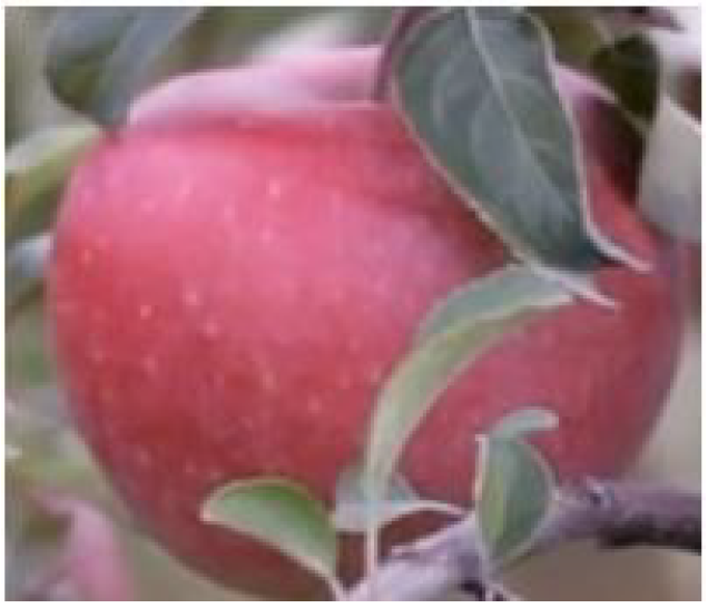
Table 4.
Different cases that affect the appearance of an apple that we include in our training dataset.
Table 5.
Results of the proposed pipeline running on a video clip of apples. We show the predicted count versus the actual count and compute the L1 Loss and Accuracy. The accuracy was low with the pretrained weights due to a significant overcount. Our correction mechanism substantially improved the accuracy, however fine tuning the weights led to the best performance.
| Metrics | Pretrained | Pretrained and Corrected | Finetuned |
|---|
| Predicted/Ground Truth | 523/342 | 299/342 | 313/342 |
| L1 Loss | 181 | 43 | 29 |
| Accuracy | 47.06% | 87.43% | 91.5% |
Table 6.
Results of the proposed pipeline running on a video clip of three neighboring rows of apples. We observed consistent performance across the three rows, with accuracy varying between 90–95%. This is consistent with the performance shown on the smaller scale apple detection in the earlier experiment.
| Metrics | Apple Row 1 | Apple Row 2 | Apple Row 3 |
|---|
| Predicted/Ground Truth | 4375/4827 | 3647/3921 | 3530/3683 |
| L1 Loss | 452 | 276 | 153 |
| Accuracy | 90.6% | 93.0% | 95.8% |
Table 7.
Results of the proposed pipeline running on a video clip of pumpkins and oranges. The oranges are counted using pretrained YOLO weights and thus produce a lower accuracy of 79.3%. Since pumpkins are trained specifically on aerial views of pumpkins, including a sample from the experiment video, the accuracy was quite high.
| Metrics | Pumpkin Counting | Orange Counting |
|---|
| Predicted/Ground Truth | 219/233 | 96/121 |
| L1 Loss 1 | 14 | 25 |
| Accuracy | 93.9% | 79.3% |
Table 8.
All of the assigned containers are fully utilized. Note that while the last container has 77% utilization, this is because the remaining number of apples was 230 at that point, not 300, so 77% is the maximum utilization the container can reach.
Table 8.
All of the assigned containers are fully utilized. Note that while the last container has 77% utilization, this is because the remaining number of apples was 230 at that point, not 300, so 77% is the maximum utilization the container can reach.
| Latitude | Longitude | Utilization of Container |
|---|
| 43.91716 | −78.62771 | 100% |
| 43.91732 | −78.62776 | 100% |
| 43.9174 | −78.62782 | 100% |
| 43.91757 | −78.62788 | 100% |
| 43.91774 | −78.62796 | 100% |
| 43.91786 | −78.628 | 100% |
| 43.91805 | −78.6281 | 100% |
| 43.91818 | −78.62814 | 100% |
| 43.91833 | −78.62821 | 100% |
| 43.91853 | −78.62829 | 100% |
| 43.91865 | −78.62834 | 100% |
| 43.91872 | −78.62838 | 77% |
Table 9.
None of the containers have 100% utilization due to the maximum distance restriction, however they’re still fairly highly utilized, thus no containers are wasted and the farmer may find this to be a favorable balance between even spacing of containers and properly utilizing the container capacities.
| Latitude | Longitude | Utilization of Container |
|---|
| 43.91743 | −78.62783 | 97.4% |
| 43.91785 | −78.628 | 80% |
| 43.91827 | −78.62816 | 76.7% |
| 43.91872 | −78.62838 | 98.9% |
Table 10.
The containers are fully utilized, however the last container is only half full and is placed too close to the 3rd container, and the other three containers have high spacing between them. This is a less favorable option for the farmer as it adds extra time and effort for the harvesters.
Table 10.
The containers are fully utilized, however the last container is only half full and is placed too close to the 3rd container, and the other three containers have high spacing between them. This is a less favorable option for the farmer as it adds extra time and effort for the harvesters.
| Latitude | Longitude | Utilization of Container |
|---|
| 43.91745 | −78.62783 | 100% |
| 43.91798 | −78.62807 | 100% |
| 43.91853 | −78.62829 | 100% |
| 43.91872 | −78.62838 | 53% |


