Abstract
Wearable sensors are widely used in activity recognition (AR) tasks with broad applicability in health and well-being, sports, geriatric care, etc. Deep learning (DL) has been at the forefront of progress in activity classification with wearable sensors. However, most state-of-the-art DL models used for AR are trained to discriminate different activity classes at high accuracy, not considering the confidence calibration of predictive output of those models. This results in probabilistic estimates that might not capture the true likelihood and is thus unreliable. In practice, it tends to produce overconfident estimates. In this paper, the problem is addressed by proposing deep time ensembles, a novel ensembling method capable of producing calibrated confidence estimates from neural network architectures. In particular, the method trains an ensemble of network models with temporal sequences extracted by varying the window size over the input time series and averaging the predictive output. The method is evaluated on four different benchmark HAR datasets and three different neural network architectures. Across all the datasets and architectures, our method shows an improvement in calibration by reducing the expected calibration error (ECE)by at least 40%, thereby providing superior likelihood estimates. In addition to providing reliable predictions our method also outperforms the state-of-the-art classification results in the WISDM, UCI HAR, and PAMAP2 datasets and performs as good as the state-of-the-art in the Skoda dataset.
1. Introduction
Extracting data from wearable sensors and converting them into meaningful information has given rise to different paradigms in ubiquitous and pervasive computing. Human activity recognition (HAR) with sensors is one such paradigm that has gained much traction in the past 15 years. HAR is the method for classifying human activities in multiple contexts. Sports [1], personal fitness tracking [2], tracking activities of daily life (ADL) [3], and geriatric care [4] are some prominent applications of HAR with wearable sensors. Popular sensors used in this domain include accelerometer, gyroscope, magnetometer, heart-rate sensor, etc. HAR with wearable sensors is a multivariate time-series classification problem. In recent years, the most popular choice for modeling human activity recognition (HAR) problems has been deep learning (DL). The expressiveness of DL techniques towards automatic feature extraction made it a popular choice among researchers to investigate their applicability to the HAR problems. Most DL architectures strive to improve primarily on predictive accuracy, i.e., they focus on detecting the activity classes correctly during test time. However, in addition to providing a correct prediction, it is also essential to produce a reliable prediction. Calibration of confidence, i.e., predicting a probabilistic estimate representing the actual likelihood, plays a crucial role in this aspect. Calibration aims to reduce the gap between the predictive accuracy and confidence estimates of the prediction. Standard neural networks trained towards accuracy are prone to producing miscalibrated confidence estimates through the softmax function. In practice, they produce overconfident wrong estimates, thus affecting the reliability of the model [5]. Although calibrating neural networks has taken off in the last couple of years in computer vision and NLP domains [6,7] it is relatively under-explored in the context of HAR with wearable sensors. This paper bridges this gap by proposing a novel neural network ensembling method for wearable sensor-based HAR.
Model ensembling is a popular technique used in machine learning for improving classification metrics [8]. An ensemble reduces variance in predictions that improve classification accuracy. A reduction in predictive variance also results in a better calibration [9]. Thus, the right ensembling strategy improves both calibration and classification.
A discretized interval of time, also called a time window, is a crucial component of an HAR process. By extracting patterns from the temporal window, the DL model can classify one activity from another. In most previous work, fixed window size and a fixed overlap are used for datasets containing different activities exhibiting different patterns in the time series. For a homogeneous dataset containing a similar type of activity, the fixed window size pattern extraction is logical. However, the one size fits all concept is counter-intuitive for heterogeneous datasets containing different types of activities. The time window needed to extract features for one activity might differ from another activity (owing to nature, periodicity, etc.). e.g., the periodicity of a running activity is different from vacuum cleaning. To extract features using the same window size from these two very different activities is sub-optimal. To overcome this problem, an input-ensemble-based novel training method, deep time ensembles is proposed. In this method, different models trained with temporal sequences extracted using different window sizes from the raw signal are ensembled. The idea is that each model of the ensemble specializes in recognizing certain genre activities that are sensitive to the input sequence created with specific window size. An ensemble thus combines the individual expert predictors to boost the overall prediction capability. Moreover, the probabilistic estimates harnessed from each model vary due to the variable window sizes. Averaging them softens the softmax output of the ensembled models, thus eliminating the overconfident estimates produced by individual softmax functions. The combined effect of variance reduction, softening of softmax, and predictive boosting through ensembling helps DTE calibrate HAR models as well as improve its classification performance.
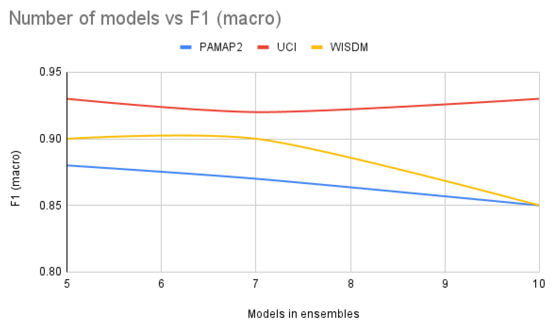
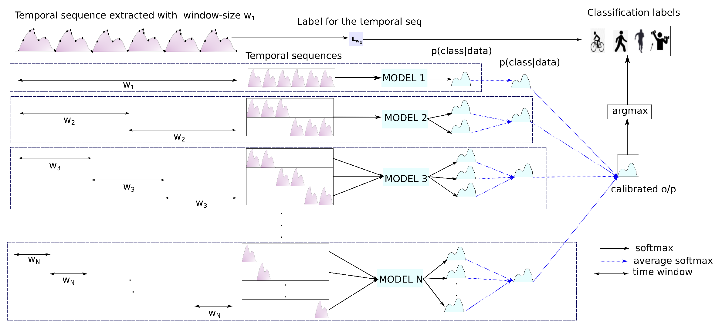
The proposed method has two main parts (see Figure 1): temporal sequence extraction, where based on a set of different window sizes, temporal matrices from the raw signal (with the window size and window overlap as hyperparameter) are extracted. In the second part ensembling, the temporal matrices are used to train individual models of the ensemble. The softmax output from each of those models is averaged to produce the final prediction.
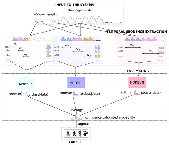
Figure 1.
Deep time ensembles: Overview.
DTE is evaluated on four public datasets, WISDM [10], UCI [11], PAMAP2 [12], and Skoda [13]. DTE can be used in conjunction with any model architecture. In this paper, three architectures were chosen, CNN, LSTM, and Convolutional LSTM. DTE improves calibration by reducing the expected calibration error (ECE) by at least for all the datasets and architectures. Moreover, it is observed that DTE outperforms the baseline models on the classification metrics for all the chosen datasets (except Skoda) by at least .
The main contribution of the paper is the proposition of deep time ensembles, a simple yet effective ensembling technique for HAR with time-series data originating from wearable sensors. The system’s effectiveness in calibrating deep learning models and improving the classification metrics was demonstrated. For calibration experiments, the state-of-the-art models were replicated and compared with DTE. The method is also compared with the standard temperature scaling recipe [14] (used for improving calibration) and reflected upon the model performance. To the best of our knowledge, no previous work explored calibration in the context of HAR.
2. Related Works
In this section, the literature is grouped into several categories, and a comparative analysis of the proposed method with respect to each group is presented.
2.1. Wearable Sensor-Based HAR Using Deep Learning
HAR from mobile and wearable sensor data have been studied using learning algorithms. Among the Machine learning methods, decision tree [15], random forest [16,17], and SVM [18,19] showed the best performance in the task; however, one of the main drawbacks of these approaches is the need for handcrafted features reliant on domain knowledge. It is often difficult to evaluate the extracted features’ efficiency since there is no defined strategy for their extraction. In addition, the procedures could be time consuming, and the extraction methods introduce assumptions about data, increasing the induction bias. In recent years, the most popular choice for modeling HAR problems has been deep learning (DL) [20,21,22,23,24]. The expressiveness of DL techniques towards automatic feature extraction made it a popular choice among researchers to investigate their applicability to the HAR problems. Naturally, a lot of robust architectures have evolved that have pushed the state-of-the-art in these problems. Due to their ability to capture temporal information, convolutional neural network (CNN) [25] and long short-term memory (LSTM) [26] based models have particularly proved to perform very well HAR with sensor data. This characteristic allows the neural networks to extract temporal features from the data using less preprocessing, thus reducing the learning bias and making the deep learning models more suitable for building end-to-end systems, facilitating both the training and recognition processes. Popular choices of deep-learning architectures for HAR encompass 1D convolutional neural networks [20], recurrent neural networks [27], including the LSTM variant, autoencoder-based architectures [28], and other hybrid solutions, such as convolutional LSTM [21]. While the deep-learning-based methods rely on a fixed window size to extract temporal sequences from time-series sensor data, DTE uses a number of different window sizes as input and trains a neural network ensemble. This helps boosting the classification metrics when compared to some previous works [6,20,29,30]. Furthermore, DTE can be used with any base neural network architecture. Table 1 presents the datasets, architecture, and macro f1-scores for some of the previous works that are chosen as baselines in this paper.

Table 1.
Dataset, architectures, and macro f1-scores of the previous works forming our baselines.
2.2. Calibration of Neural Networks
Guo et al. [14] argued that despite achieving very high accuracy the modern neural networks are poorly calibrated, affecting the reliability of the model predictions. This behavior could compromise the decision-making process in safety-critical systems. In the domain of computer vision, calibration has been explored recently [7,9,14]. To the best of our knowledge, confidence calibration of predictive output has not been explored in HAR previously. The devised method adapts calibrating DL models used in sensor-based HAR procedures. This improves the reliability of the models by generating predictions that represent the true likelihood.
Many approaches were proposed to adjust the model calibration, from tuning the model capacity, weight regularization, and batch normalization to stand-alone methods that require a hold-out validation set for hypertuning. Among the latter, two main families of algorithms can be identified, inspired by histogram binning or Platt scaling [31] algorithms. The first family includes histogram binning [32], isotonic regression [33], and Bayesian binning into quantiles (BBQ) [34]. The second one contains matrix scaling and temperature scaling [14]. All these methods require an extra post-processing step. DTE can be used to calibrate predictions from time-series (in this paper for HAR)-based neural network models.
2.3. Ensembling
Inspired by ensembles used in uncertainty estimation [35], DTE is formulated that achieve well-calibrated confidence estimates without any extra post-processing. While ensembles have been used previously in the context of classification [36,37], the research closest to our work can be found in Guan et al. [6]. They propose an ensemble of LSTM learners to achieve HAR; however, the window-size selection for temporal sequence extraction is different compared to our method. Additionally, our primary goal is to explore model calibration, which was not taken into consideration by [6].
3. Methods
In this paper a supervised time-series classification problem is addressed. Our objective of calibration is similar to that of [14]. The input data are x, and the corresponding labels are y. A neural network f, parameterize the distribution . The confidence of the predictions is given as P. A calibrated output is desired, such that it represents the true probability. By producing a calibrated output, the gap between the accuracy and mean confidence of the model is also reduced. For a perfectly calibrated model, for mean confidence of 0.8, a mean accuracy of 0.8 is expected.
To visualize calibration reliability diagram is used [38]. The reliability diagram representation is adopted from [39]. In these diagrams accuracy is plotted as a function of confidence (see Figure 5a). In the upper part of Figure 5a the confidence is represented in the x-axis and accuracy is represented in y-axis. Furthermore, the x-axis is divided into fixed number of intervals (10 in this case). Predictions that fall in the confidence interval are assigned to that bin. After assigning the predictions, the mean confidence and the mean accuracy of the individual bins are calculated. For a multi-class classification problem, the accuracy of each bin is given by,
and the average confidence of each bin is defined as,
where n is number of samples in each bin, and is the bin number. The bold black line represents the accuracy of each bin in the confidence versus accuracy plot (top part of the diagram). The bars represent the difference between the accuracy and the confidence in each of the bins. The lower part of the reliability diagram displays the histogram of the samples assigned to each bin and helps understand the importance of calibration in each of the bins. e.g., in Figure 5a most of the samples are concentrated in the last bin, and the calibration of that bin has more impact on the overall calibration. These two boxes, when seen in conjunction, provide us with a holistic understanding of model calibration. An identity function is plotted for a perfectly calibrated model (denoted by the diagonal line on the upper part). The miscalibration is represented by deviation from the perfect diagonal.
While reliability diagrams are a visual explanation towards calibration, expected calibration error (ECE) is a metric-based representation of the same. Motivated by the fact that miscalibration is the difference between confidence and accuracy, ECE captures the weighted average difference of bin’s accuracy and the confidence score. It is given as:
where M is the number of bins and N is the number of samples.
3.1. Ensembles and Model Calibration
There is an intrinsic connection between predictive variance, accuracy, and calibration. In their work, Seo et al. [9] showed that predictive variance is inversely proportional to both calibration and accuracy. A good ensembling regime helps to reduce the variance in prediction and boost the predictive performance [40]. Thus, it is hypothesized that reducing predictive variance through ensembling helps model calibration and classification. In comparison with temperature scaling [14], a popular calibration method, ensembling does not require any extra post-processing round.
Furthermore, traditional neural networks trained towards softmax are prone to be miscalibrated. This is primarily attributed to the overestimated probability assignment of the positive class by the softmax function [5]. Using these neural network models can result in overconfident probability estimates at the output. Ensembling, equivalent to Bayesian model averaging, helps to incorporate uncertainty in the data effectively [35]. In ensembling, the softmax output from individual models is softened through averaging, mitigating the overconfident outputs of individual models. Hence, a well-calibrated probability distribution is obtained at the output. This is reflected in the predictions as well. The observations about ensembling led us to devise a novel ensembling method fit for time-series-based HAR called deep time ensembles (DTE).
3.2. Deep Time Ensembles
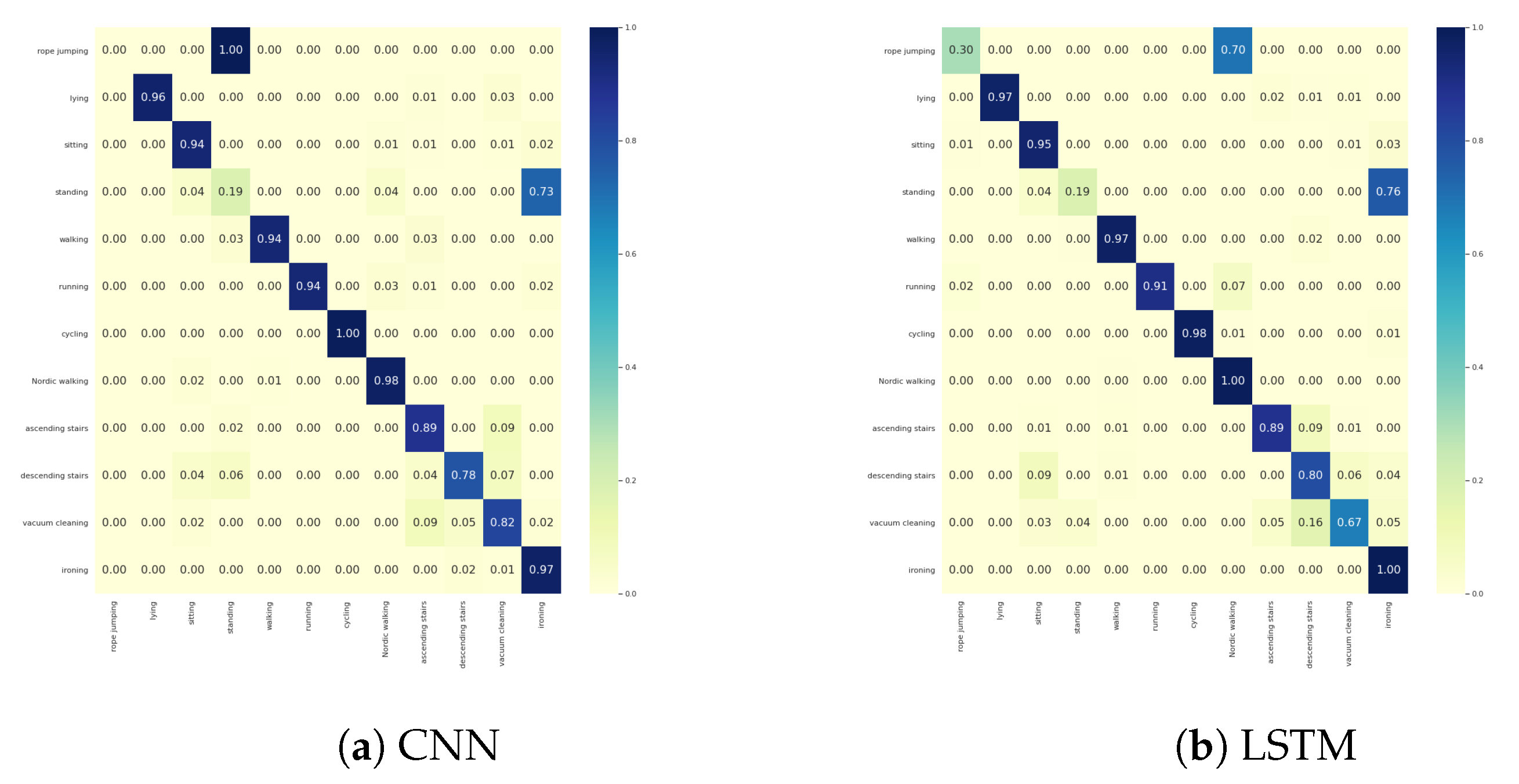
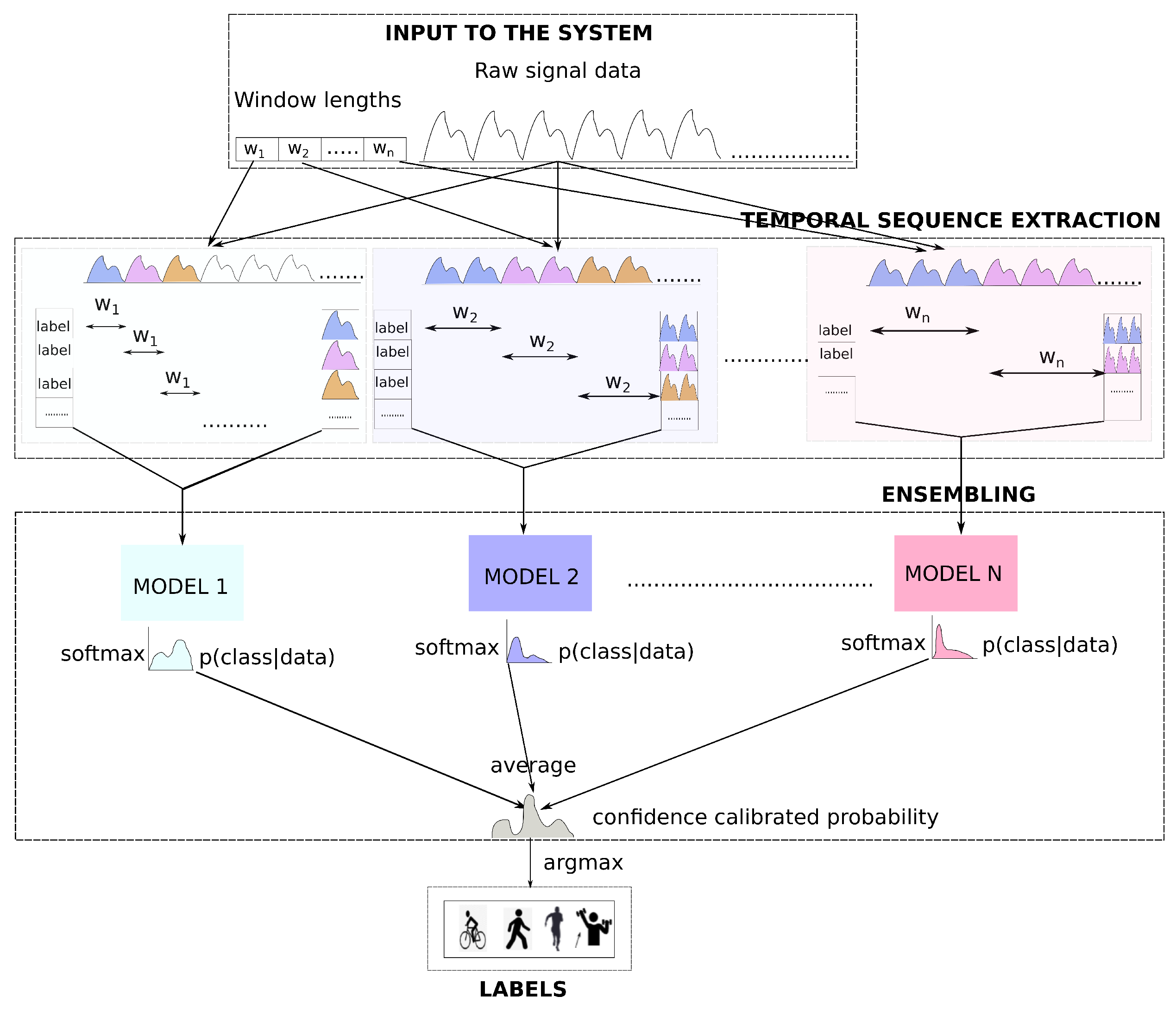
Time series recordings have the structural information encoded into their temporal order. The data fed into the model are strictly ordered by the acquisition time. The scope of exploration depends explicitly on the number of consecutive values fed into the model. Hence, extracting the temporal information is highly dependent on the window size of sensor readings and the overlap between the consecutive windows. These two hyperparameters influence the order of dependencies between empirical values explored by the model. Traditionally in activity recognition, temporal sequences are extracted from raw time-series signals using a fixed window size. These temporal sequences and their corresponding labels for each sequence are used for training the deep learning models. For datasets that consist of homogeneous activities, i.e., activities that exhibit similar patterns in their signal representation, a fixed window size might suffice; however, in datasets with a wide range of dissimilar activities, the fixed window size is sub-optimal. In Figure 2, the chest accelerometer data of four activities (out of twelve) from the PAMAP2 dataset for a single subject are plotted.
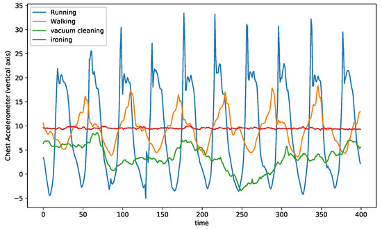
Figure 2.
Comparison among three activities from PAMAP2 dataset.
On the one hand, the running and walking activities have a visible periodicity. On the other hand, the vaccum cleaning activity has much less evident periodicity, while the ironing activity has almost no periodicity. While for the running and walking assuming a window size equal to the period or two periods of the activity for temporal sequence extraction, it might be the right choice for the DL model; however, the same window size is rather long for pattern extraction of a static activity such as ironing. Similarly, vaccum cleaning requires a different optimal window size. Thus, each activity in the same dataset is sensitive to a different choice of window size that benefits the learner.
Based on the above observation and our goal of calibrating HAR models with an ensemble, the deep time ensembles method is proposed. In our algorithm, temporal sequences from the same input signal using different window sizes is extracted. For each window size a collection of temporal sequences form the temporal matrix. Thus multiple temporal matrices are extracted with multiple window sizes. With the extracted temporal matrices, an ensemble of models is trained (one model per temporal matrix). Each model in the ensemble would be expert at recognizing certain activities, and the combination of all would be beneficial for the overall HAR model. Creating an ensemble with fixed window-size duration would provide a limited amount of temporal information conveyed to the model, and DTE is superior in that aspect. Furthermore, the extraction of temporal sequences with different windows size allows us to model the uncertainty beyond the length of window size. Eventually, by averaging the predictive response over the ensemble, it is possible to model the uncertainty that depends solely on the recordings and no other hyperparameter (i.e., window size). The promotion of such coherent (recording) uncertainty helps mitigate the overconfidence that might come from the softmax distribution of a single model. This, in turn, helps to calibrate the likelihood coming out of the ensemble.
DTE has two main steps
- Extracting temporal sequences from the time series (See temporal sequence extraction module of Figure 1) based on a set of different window sizes.
- Training ensembles based on extracted temporal sequences (See ensembling module of Figure 1).
The goal of the machine learning method is to determine the activity given a sequence of the wearable sensor signal. As seen in Figure 1, there are two inputs to our system, the raw signal data, originating from sensors, and an array of window sizes to extract temporal sequences for individual models of the ensemble. The overlap between windows is another input to our model, but it is considered as a fixed value for the method and is omitted in the diagram. The same data serve as input for each block inside the temporal sequence extraction module. In the first block, a sliding window of size is selected and slided over the raw signal data continuously until the data expire. For each slide of , extract temporal sequences from the raw time-series data are extracted. All those temporal sequences (until the end of the data) are appended to form a temporal matrix. There is a related activity for each temporal sequence, and the extracted labels for all temporal sequences form the label vector. Similarly, a window size of is used for the next block and this creates another set of temporal matrices and label vectors. In this way, temporal matrices up to are extracted. For each of such temporal matrices and the corresponding label vector, a neural network model (with the architecture of our choice) is trained in the ensembling module. During the prediction/evaluation, the softmax distribution output from each model of the ensemble is averaged. The averaged distribution is a confidence-calibrated one, and the index of the maximum value of the distribution gives us the activity label.
Algorithmically, DTE is divided in two phases, the training phase and the evaluation/prediction phase. The training phase happens following the temporal sequence extraction. Once individual temporal matrices and label vectors are extracted for each selected window size, the training is similar to any other DL method. The algorithm is presented in Algorithm 1.
| Algorithm 1 Deep Time Ensemble—Training |
|
There are specific considerations that are required while performing an evaluation/prediction with DTE (depicted in Figure 3). In the diagram, a single temporal sequence extracted with window size is presented. For the sake of convenience, it is called . The temporal sequence consists of recorded sensor points. There are N models pre-trained with temporal matrices and labels extracted with windows, where . While training and evaluating, each temporal sequence of all the temporal matrices is associated with a single label. In the demonstrated figure, the label index for the temporal sequence is given as . For the window size , the whole temporal sequence is fed to the model (MODEL 1 in the figure) trained on a temporal matrix created with . Using window size , two temporal sequences from can be extracted. Both these temporal sequences are used to generate two softmax distributions from MODEL 2 that are averaged out as a single distribution. In the diagram, overlapping windows are omitted for the sake of simplicity.
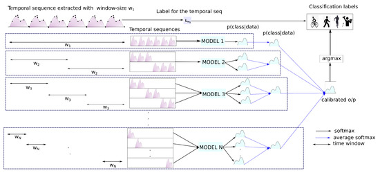
Figure 3.
Magnified view of DTE evaluation for one temporal sequence.
Similarly for , three temporal sequences are extracted from , and an averaged softmax is extracted from the MODEL 3. The process is continued all the way up to , the smallest window size. Finally, the single distributions that are obtained earlier are averaged to output the confidence calibrated probabilities. During the evaluation, the label corresponding to the index of the maximum value of the distribution is evaluated with the actual label . While in a live-system the confidence calibrated output can be provided as the result. The Algorithm 2 extends the same concept to multiple temporal sequences or a temporal matrix extracted with window size .
| Algorithm 2 Deep Time Ensemble—Evaluation/Prediction |
|
The novelty of this paper is two-fold:
- Dissimilar activities are associated with different time windows instead of a fixed one as proposed in most of the earlier works. This led to devising DTE that ensembles different temporal representation of the same input signal.
- The observation that the ensembled model also calibrates the predictive output. This in turn results in predictions that represents the true likelihood.
In the next section an extensive evaluation of DTE is presented that justifies the mentioned formulations.
4. Evaluation
To validate the effectivness of our method in calibrating HAR models, a range of experiments were conducted on four datasets, namely PAMAP2, UCI, WISDM, and Skoda. For the experiments, three neural network architectures were chosen, namely CNN, LSTM, and convolutional LSTM (discussed in methods). The architectures for each were chosen so that they match the previous works that are compared with this paper, and they are presented in Table 1. The previous works and the corresponding architectures are replicated to form a baseline for comparison with DTE. Primarily, DTE is evaluated on three factors.
- How does DTE fare in calibrating neural network models?
- How does DTE compare with the popular temperature-scaling [14] method of calibration?
- How does DTE compare with the previous work in the downstream classification task?
To evaluate the calibration, the standard metric is expected calibration error (ECE), as defined in the methods section. In particular, we strive for a lower value of ECE, since it means that the predictions are more calibrated or representative of the true probability. The metrics used for evaluating the classification performance of our method are accuracy, macro f1 score, and average f1 score. In rest of the section: the datasets are described first, followed by model configuration, then the calibration results are discussed followed by classification performance.
4.1. Datasets
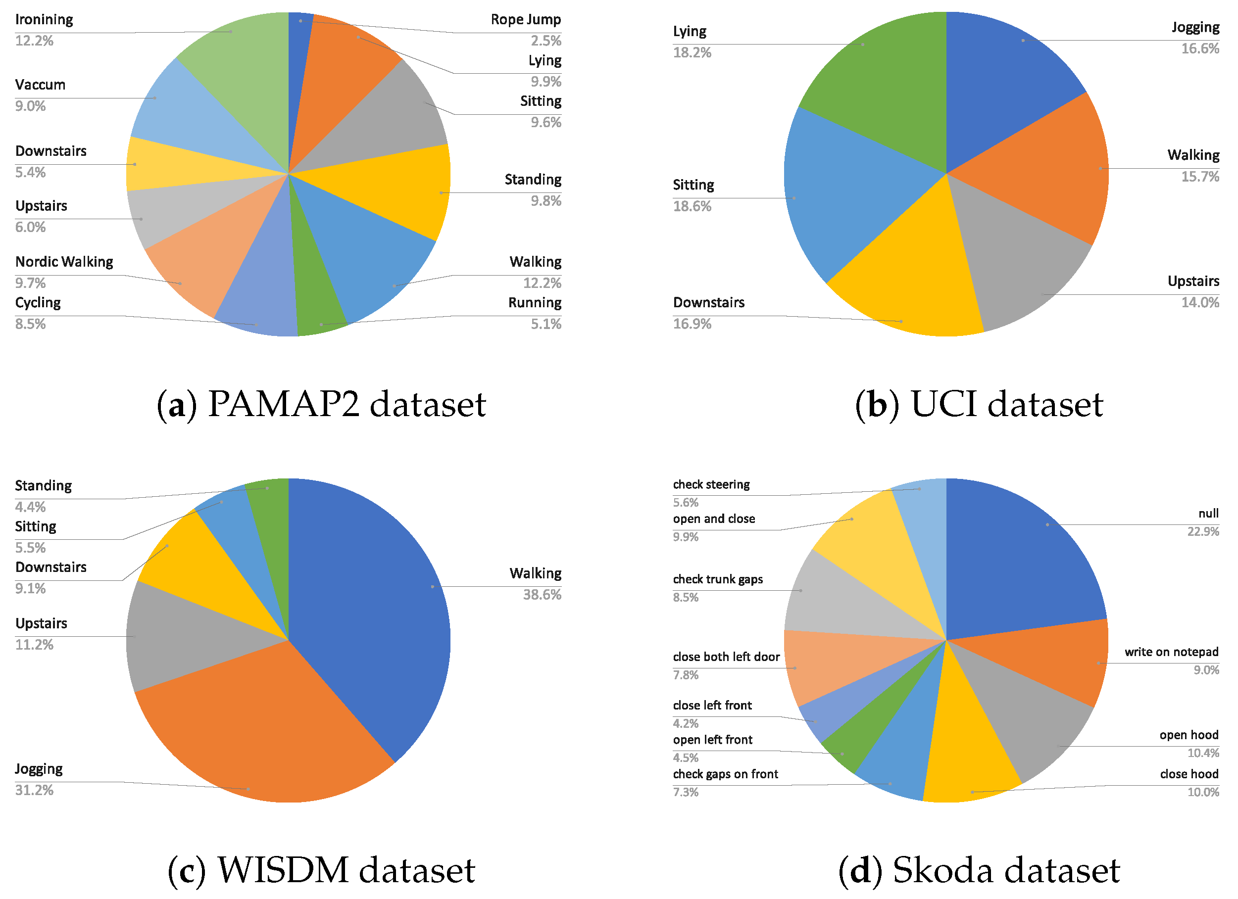
The chosen datasets consist of a good mix of different activities and sensor modalities. The class distribution of the activities in each dataset is shown in Figure 4. Next, the specifics of each of the datasets are highlighted.
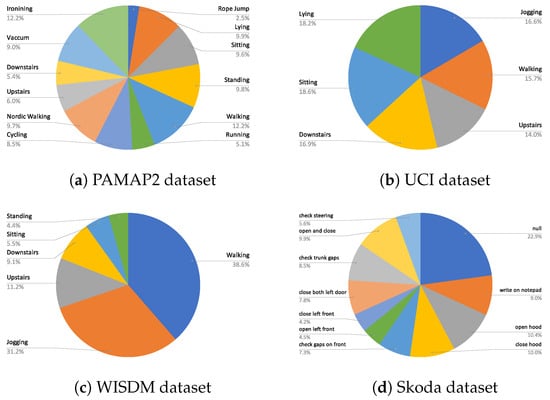
Figure 4.
Class distribution of (a) PAMAP2, (b) UCI, (c) WISDM, and (d) Skoda dataset.
- WISDM dataset:WISDM dataset [10] consists of 36 subjects and 6 activities, namely standing, sitting, downstairs, upstairs, walking, and jogging. The activities were recorded with a tri-axial accelerometer sensor. The training, validation, and evaluation splits for the WISDM dataset are adopted from [20,29]. Users 1–24 form training data, 24 and 25 form the validation data, and 26–36 are used for testing. After preprocessing and windowing of the test split, 3026 test samples for evaluation are obtained.
- UCI dataset: The UCI dataset [11] is a public dataset consisting of six activities lying, standing, sitting, downstairs, upstairs, and walking recorded from 30 subjects. The dataset was recorded with a triaxial accelerometer and gyroscope, resulting in six dimensions. Similar to the WISDM dataset, the training, validation, and testing split of this dataset was also adopted from [20]. After preprocessing and windowing, the number of test samples for evaluation is 2993.
- PAMAP2 dataset: The PAMAP2 dataset [12] consists of 12 activities recorded from nine subjects for over 10 h. It consists of sporting activities, activities of daily life, and other domestic activities. It consists of a wide array of multivariate sensor data (accelerometer, gyroscope, magnetometer, heart rate, etc.), resulting in 52 dimensions. The training, testing, and validation dataset was extracted following the protocol of [30]. Runs 1 and 2 from subject 5 is the validation set, and runs 1 and 2 from subject 6 is the testing set. The rest of the data were used for training. Guan et al. [6] did a thorough sample-wise evaluation on the PAMAP2 dataset in their work. To accommodate a similar evaluation strategy, testing samples from the testing dataset with complete overlap are extracted. This gives 83 K samples for testing. These samples are used to evaluate our method with both [6,30].
- Skoda dataset: The Skoda dataset [13] is comprised of a collection of 10 manipulative gestures/activities of a factory worker working in the assembly line of a car manufacturing process. The worker wore 20 3D accelerometer sensors. The training/validation/testing splits of the Skoda dataset are adopted from [21]. To create test samples same overlap as training is assumed.
For DTE, there are multiple window sizes that are used to extract temporal sequences from the same input signal. This leads to different sizes of training and label samples for each model of the ensemble. In Table 2, the number of temporal sequences that are extracted from the same dataset, for different window sizes is presented.
Table 2.
Number of temporal sequences and labels (for training) per dataset for each model in the ensemble.
4.2. Model Configuration
In this work, a baseline neural network model was chosen, DTE was applied to it, and the baseline was compared with its DTE variant. The neural network model configurations were chosen from previous works and became baselines for making a fair comparison. For PAMAP2 dataset, the CNN configurations from [30], and the LSTM configurations from [6] were adopted. For the UCI dataset, the model parameters of CNN were chosen from [20]. Although [20] added an extra feature layer as concatenation in their work, it is omitted in our baseline. This is to keep the feature extraction procedure as automated as possible. For the LSTM architecture of the UCI dataset, a two-layer LSTM with 128 neurons in each cell is selected. The LSTM configuration of the WISDM dataset was chosen from [29], and for the Skoda dataset, the convolutional LSTM architecture has the same parameters as [21]. Table 1 lists the baseline models that were considered for applying DTE. Throughout, the evaluation the results of calibration and classification on these architectures are presented. The details of the architectures and hyperparameters are presented in Appendix A.
4.3. Calibration Results
To the best of our knowledge, no previous experiments on the calibration of neural networks on HAR were showcased. Hence, the previous works stated in Table 1 are replicated and the ECE metric is calculated by adding the calibration module to the replication. The previous works are called baseline models for the rest of the section.
4.3.1. ECE and Reliability Diagrams
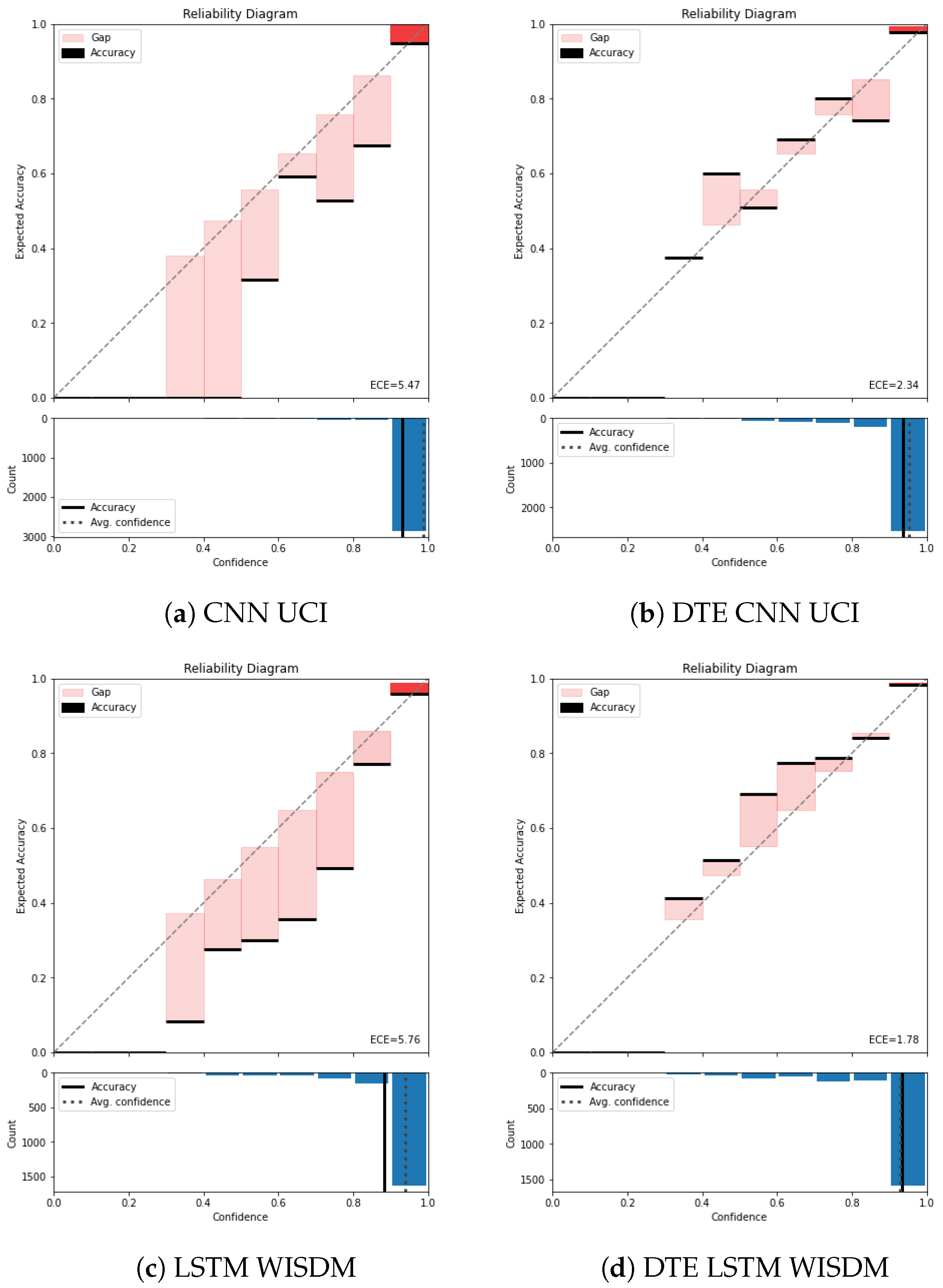
As discussed earlier, the standard measure of calibration is ECE. An essential factor for calculating ECE is selecting the number of bins over which the metric will be calculated. The number of bins were chosen to be 10 () across all the experiments and architectures for our experiments. The calibration result is reported in Table 3. In this table, the ECE for all the baseline architectures and the corresponding DTE variants for each dataset are presented. All experiments were run 10 times for robustness and the mean and the standard deviation on the metrics are shown. From Table 3 it is observed that the baseline model for PAMAP2 dataset adopted from Hammerla et al. [30] has an ECE of 0.06, while applying DTE on it decreases the ECE to 0.03. This drop in ECE indicates an improved calibration. Similarly, across all the dataset and architectures, DTE improves calibration by at least . The visual aid for understanding calibration is a reliability diagram. The reliability diagrams for the baselines and DTE for all the datasets are plotted. e.g., in Figure 5 the reliability diagram for the UCI dataset for the chosen architectures (CNN and LSTM) is presented.
Table 3.
Classification and calibration results (10 experiments per setting) for baseline architectures versus DTE (our method) across all datasets.
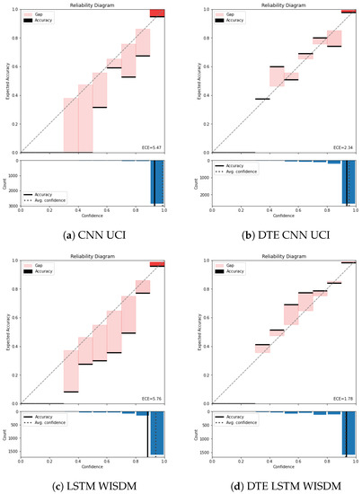
Figure 5.
Reliability diagramUCIandWISDM: Without temperature scaling. The top half of each reliability diagram (a–d) has confidence in the x-axis and accuracy in the y-axis. The x-axis (confidence) is divided into 10 bins. The colored bars represent the difference between mean accuracy and the mean confidence of the samples that falls in those bins. The black line on top or bottom of each bar represents the accuracy of the samples in that bin. The bottom half of the reliability diagram represents the histogram of the samples concentrated in each bin. The ECE is calculated be averaging the difference between confidence and accuracy across all the bins.
Color temperature is used to denote the gap bars (difference between confidence and accuracy) based on the number of samples residing in each bin. In Figure 5a it is observed that the baseline CNN model is highly confident about most of the predictions and has put most of the examples in the highest bin (between 0.9 and 1).
The average confidence of this model is almost (seen by the dotted line in the lower part of the reliability diagram), while the accuracy is approximately . This gap between the average confidence and the average accuracy represents the miscalibration of the model. The average binned miscalibration is captured through ECE value of . Meanwhile in Figure 5a, on applying DTE with the same architecture results in a substantial drop in ECE to . It is also noted that the gap between accuracy and the confidence in the lower part of the reliability diagram has reduced. Zooming into the highest bin for both the baseline model and the DTE variant highlights that the gap between accuracy and the confidence is lower in the DTE variant compared to the baseline CNN. This is also observed for LSTM variants of UCI dataset (Figure A2a,b)
Another observation is that DTE distributes test examples from the highest bin to the lower bins through the averaging procedure. This helps in bringing down the overall average confidence of the model. This is in line with the hypothesis, DTE mitigates the overconfidence achieved by softmax through uncertainty estimation (Bayesian model averaging) and variance reduction. The best value of calibration error is observed for DTE LSTM architecture in WISDM dataset. This can be attributed to the relatively simpler neural network architecture and lower-dimensional features of the dataset (model complexity is directly proportional to calibration error [14]). The reliability diagram for rest of the datasets are in Appendix B. Across all the datasets and architectures, DTE appears to be more calibrated than the baseline models (see Table 3 for overall results and Figure A1 for PAMAP2, and Figure A3 for Skoda).
4.3.2. Binwise Calibration
Our calibration experiments showed that DTE decreases ECE for all the cases and is very well calibrated in the higher bins, where most of the examples are concentrated (depicted by the almost non-existent gap in the higher bins of the reliability diagrams of DTE); however, a good calibration regime must guarantee that all the bins are better calibrated than baseline models. Hence, it is imperative to present the results comparing the binwise calibration of the baseline models and DTE for the best architectures across all the datasets in Figure 6. The x-axis of Figure 6 is the bin number, and the y-axis is the log of ECE in each of the bin. The dotted lines show the results for all the variants of DTE, while the solid line of the same color depicts the result for the baseline model. Taking PAMAP2 dataset as an example, the solid blue line represents binwise ECE of the baseline CNN model and the corresponding DTE variant is shown in the dotted blue line. It is seen that DTE exhibits lower ECE in all the bins than the baseline. This is true for all the datasets and architectures in Figure 6. This experiment verifies that not only in the bins where most of the examples are concentrated, but DTE also exhibits a lower calibration error in all the bins.
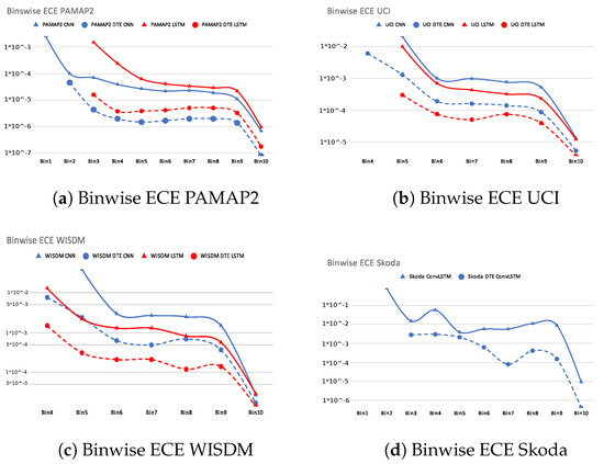
Figure 6.
Binwise ECE (along y-axis) of all datasets and selected architectures.
4.3.3. Comparison with Temperature Scaling
Apart from the comparison between DTE and the baseline model, the proposed method is also compared with temperature scaling. Specifically it is a comparison among baseline, baseline with temperature scaling, DTE, and DTE with temperature scaling. Temperature scaling is a post-processing method that aims to optimize a temperature, T based on a validation set. This T divides the softmax output and mitigates the overconfidence resulting in better calibration. To soften the softmax output, T must be greater than 1. The initialization of the T and the selection of the validation set is crucial for the optimization. If the validation set does not include all the classes, then the temperature scaling might give a sub-optimal solution (T < 1). The process is also very sensitive to the initialization of T. Following the initialization scheme found in the implementational details of the paper [14], the chosen temperature is . With this temperature value and an optimal validation set, the softmax output of the baseline model and DTE is smoothed for our best architectures for all the datasets. The results are presented in Figure 7. With temperature scaling the baseline models were successfully calibrated; however, the scores indicate using only DTE results in better calibration than baseline with temperature scaling. With temperature scaling on the output of DTE, calibration only improved for the UCI dataset. For the rest of the datasets and architectures, DTE proved to be the optimal choice for achieving the best calibration.
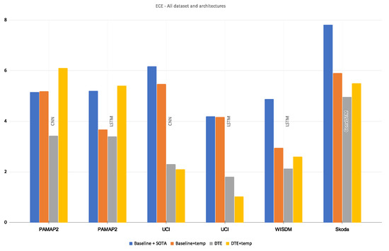
Figure 7.
Comparison of ECE (along y-axis) between baseline, baseline + temperature-scaled, DTE, DTE + temperature-scaled models.
This means that for most of the DTE models, suboptimal temperature values were reached through the optimization. This leads to a logical question about whether a different temperature initialization was required per model in the ensemble. This question is out-of-scope for this work; it can be explored in the subsequent extensions of this method. While temperature scaling is a popular method, the experiments show that DTE alone can calibrate effectively. Moreover even temperature scaling is used, it performs best when combined with DTE The reliability diagrams of temperature scaled variants are presented in Appendix B.
4.4. Classification Results
Since HAR processes are primarily concerned with classification, it is essential to justify calibration while keeping the classification performance as good as possible. The classification results of the adopted baselines and the corresponding DTEs are presented in Table 3. A comparison between the baseline model and its DTE variant per dataset (e.g., CNN versus DTE CNN, LSTM versus DTE LSTM) is made and the best metrics for the whole dataset are highlighted. Furthermore, the class-wise F1-score for two datasets (rest are presented in Appendix B) are in in Figure 8.
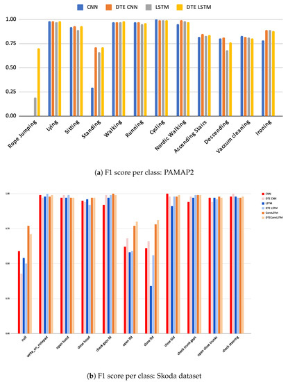
Figure 8.
F1 scores per class for PAMAP2 and Skoda dataset.
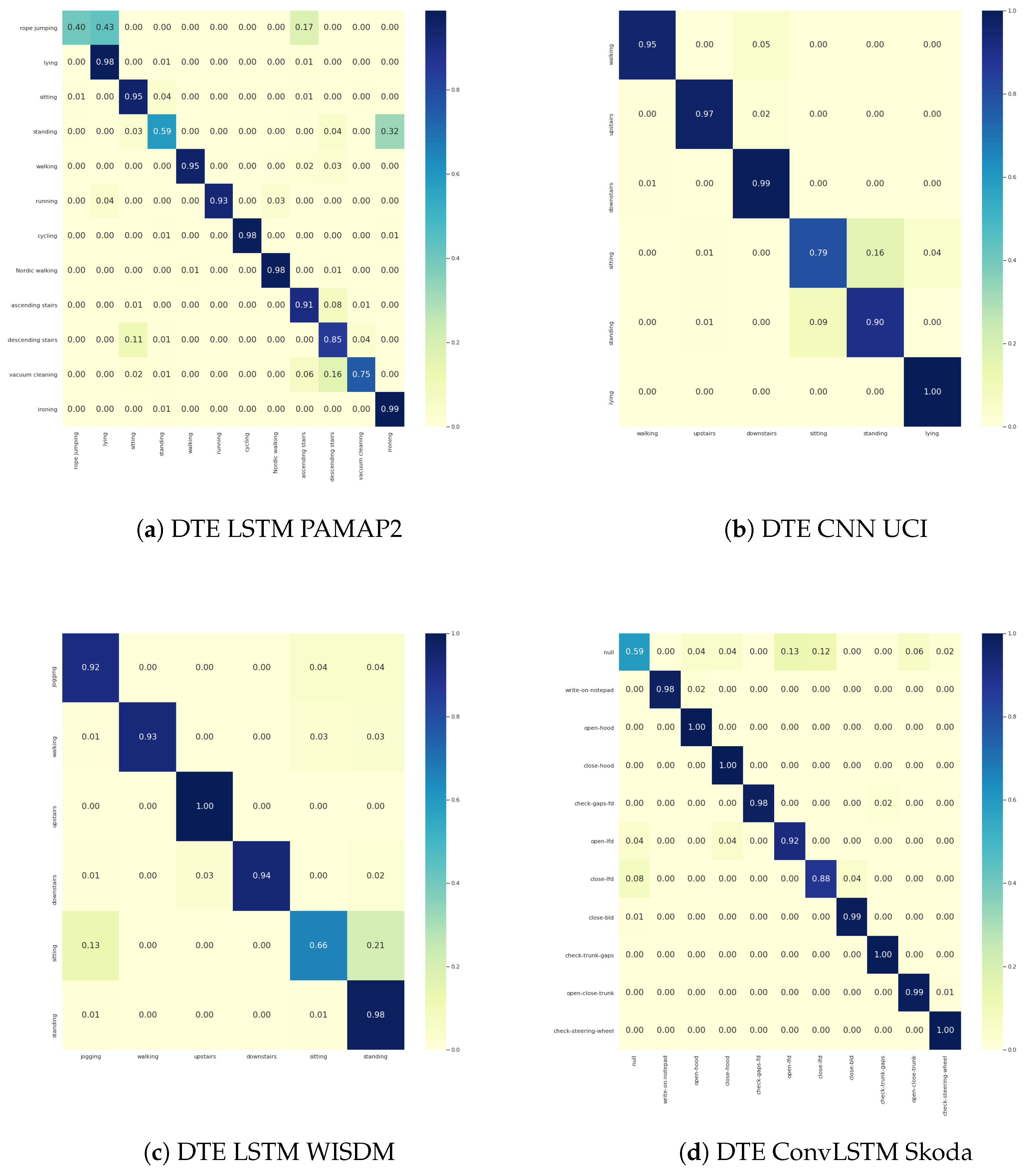
The confusion matrices of the best-performing DTE variants per dataset are presented in Figure 9. For the sake of brevity, the rest of the confusion matrices are in the Appendix section. Analyzing the classification results exposes several exciting facts about DTE. From Figure 3 it is evident that every DTE variant consistently outperforms the baseline variants in all classification metrics across all the datasets (except F1 in ConvLSTM architecture of Skoda).
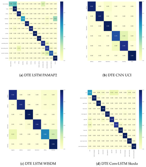
Figure 9.
Confusion matrices for best DTE architectures.
This consolidates our argument that incorporating multiple models trained with different temporal matrices as an ensemble improves the classification performance. Unlike [6], the window sizes are selected in a non-random fashion. Although this has a manual constraint, our method ensures that each base model is a strong learner for a certain set of activities and performs adequately for the rest.
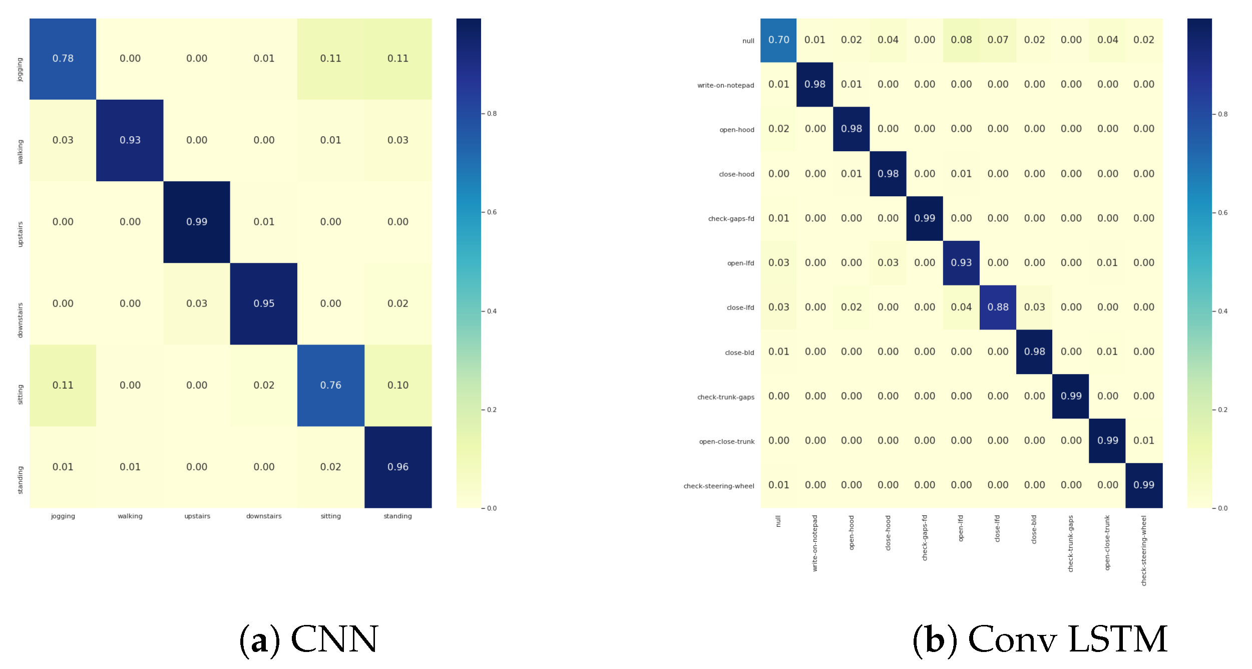
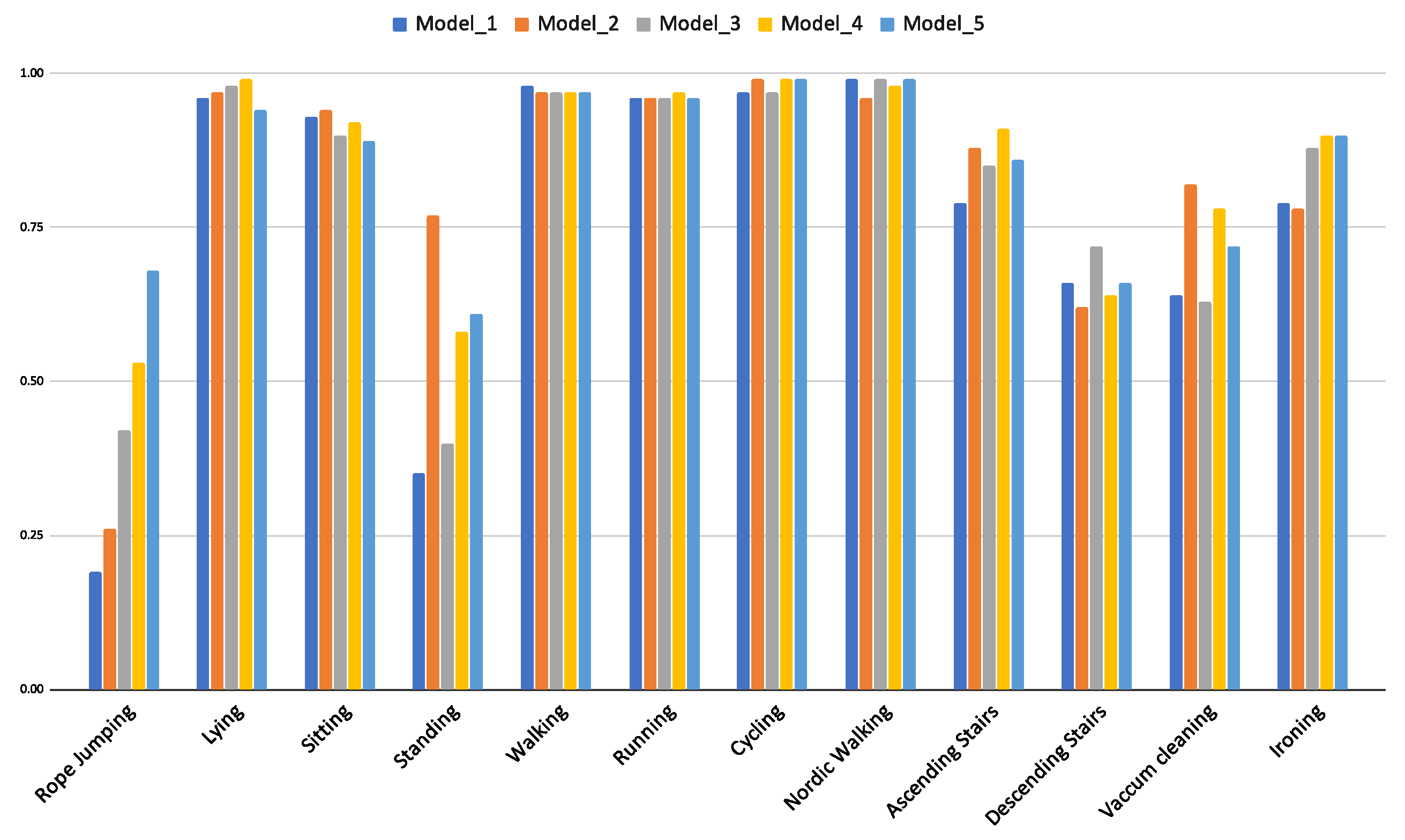
The idea of individual expert models contributing to the overall classification performance is demonstrated with an experiment where five individual models of DTE LSTM trained on PAMAP2 dataset are compared. Figure 10 demonstrates how each of the five models that are created with ascending window sizes (5 s to 9 s) perform in detecting individual activities. Thus, Model_1 is trained with temporal sequences obtained using window-size of 5 s, Model_2 with temporal sequences obtained using window-size of 6 s and so on, up to Model_5 that is trained on sequences acquired using window-size of 9 s.
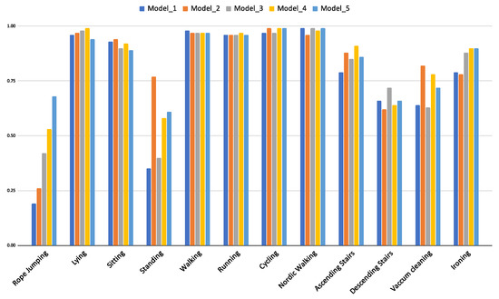
Figure 10.
F1-score of activities per model that are trained on different window sizes in DTE using LSTM architecture for PAMAP2 dataset.
The rope-jumping activity is best detected by Model_5, but it is outperformed in detection of the standing activity by Model_2. Thus, it can be inferred that no single model is an expert in detecting all the activities, rather a combined predictor is the optimal choice to detect all activities (evident from overall classification results in Table 3).
In the PAMAP2 dataset it is observed that accuracy and F1 for CNNs and LSTMs are almost equal and the F1 is substantially better in the LSTM variants. It is important to note that the rope-jumping class in the PAMAP2 dataset is underrepresented (2.5% of the training data and 0.1% in testing data). This class is not captured by CNN or its DTE variant but by both the LSTM variants (in Figure 8a). Since F1 makes a weighted average calculation, this class being significantly less in number is obscured by the better predictions of the other classes; however, F1 is a non-weighted average of the F1-score, and the inability of a model to capture one class is amplified with this score. Thus, the CNN models that cannot capture this exhibit a lower F1 compared to the LSTM models. Hence, for this dataset, F1 captures the accurate picture, and DTE LSTM outperforms all other baselines by at least .
For UCI dataset performances of DTE variants of CNN and LSTM architectures are similar, with DTE CNN outperforming the DTE LSTM by in accuracy. The classwise f1 scores (see Appendix C) show that DTE CNN detects the running and downstairs activity better than the other variants. In this dataset, DTE improves the baselines by at least . Considering the baseline metrics were already high (>0.91), this improvement is substantial. Furthermore, as stated in the earlier section, the predictions are more calibrated in the DTE variants.
WISDM dataset exhibits similar classification trends as the UCI dataset; however, the performance gains are more significant in this case. The class-specific scores show that DTE variants outperform the baseline models in all classes except sitting where the LSTM baseline has slightly better score than DTE LSTM.
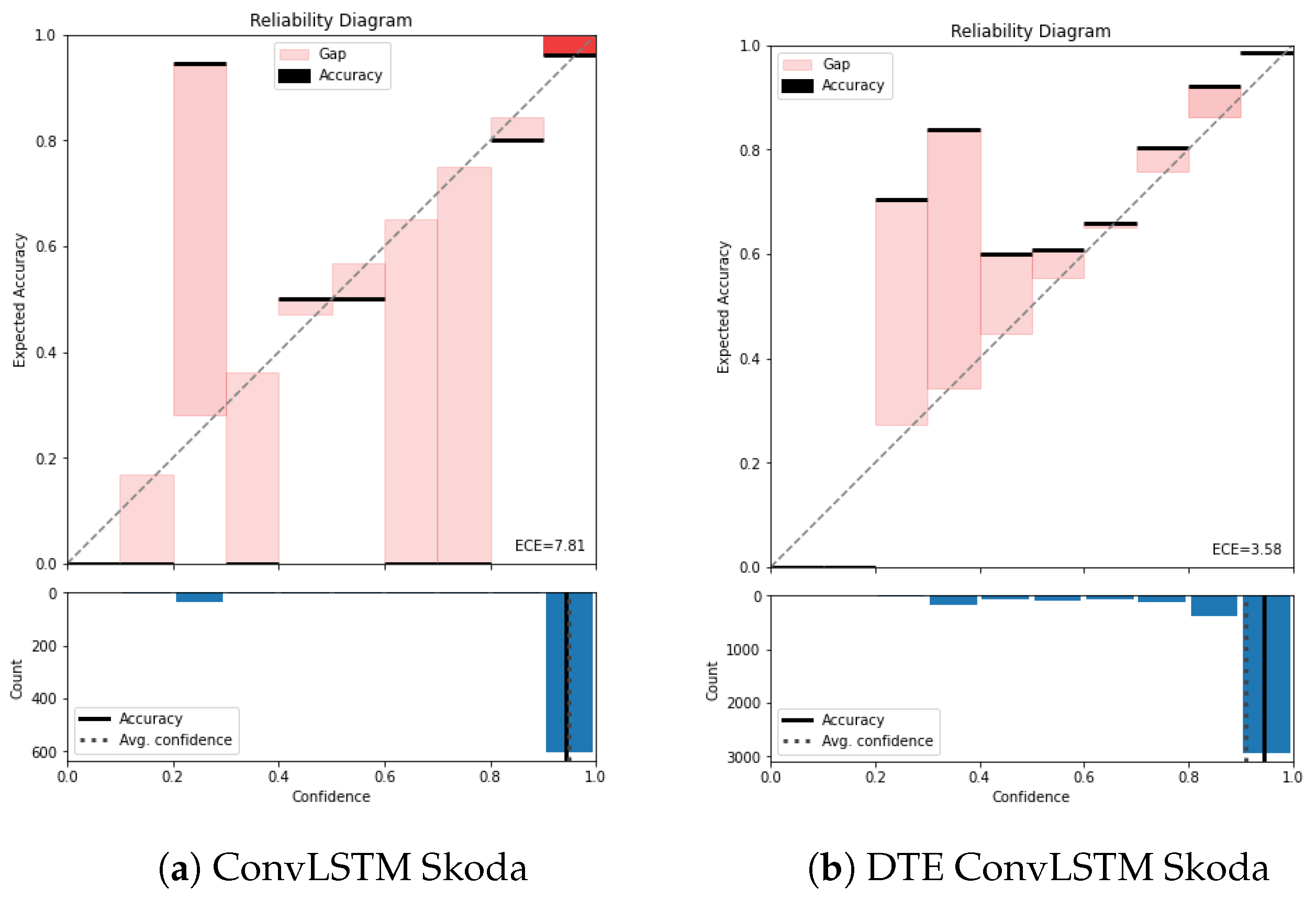
Among the three baseline architectures for Skoda dataset, the ConvLSTM architecture and its DTE outperform all others by at least in all classification measures; however, unlike other datasets and architectures the DTE variant (DTE ConvLSTM) does not improve all the metrics of the baseline. The substantial presence of null class and its detection by ConvLSTM architecture result in a better F1 (see Figure 8b) than DTE ConvLSTM. DTE is based on the idea that if the dataset consists of a wide range of different activities, each model would have the expertise to capture a specific genre of those activities. The ensemble, when combined, becomes an expert at recognizing all. A close observation reveals that the activities of the Skoda dataset in Figure 4 are somewhat similar; thus, the hypothesis that each model extracts specific class patterns through different temporal sequences is not very strong. This might be another fundamental reason that DTE exhibits lower score in F1 for the ConvLSTM architecture in Skoda. Among the rest of the architectures in Skoda, DTE variants outperform the baseline variants.
Overall DTE improves the baselines in classification performance and produces well-calibrated predictions that are much more representative of the true probability. It also validates the hypothesis that datasets with a wide range of activities (PAMAP2) benefit the most from the incorporation of DTE. Our range of experiments also provides a soft guideline for architecture selection for different datasets—e.g., in PAMAP2 and WISDM, DTE LSTM has best classification results, while for UCI, DTE CNN outperforms the rest and for Skoda, both ConvLSTM and its DTE variant performs equivalently. In cases where the baseline models are not beaten by DTE, the performance is almost similar but with better calibration. This resonates with our initial promise of providing good classification performance with well calibrated predictions.
4.5. Comparison with Standard Ensemble Models
While comparison with previous works demonstrated the effectivity of DTE, most of the compared methods (except [6]) were non-ensemble methods. Hence, for a more fair comparison DTE is compared with a neural network ensemble created with standard architectures (LSTM, ConvNets, etc.). The ensembling strategy adopted is similar to the ones in [35]. The neural network architecture is ensembled in the same parameter space, and the number of models is kept the same as the number of input window sizes in DTE. The results of the experiment are presented in Table 4.
Table 4.
Classification and calibration results (10 experiments per setting) for comparing standard ensemble versus DTE (our method) across all datasets and architectures.
From the table it is evident that across all architectures and datasets DTE outperforms or performs as good as standard ensembling methods in terms of classification. This solidifies the argument that the combination of multiple expert models available to DTE conveys more information towards pattern recognition as compared to standard model ensembling procedures. The only exception here as well is with the Skoda dataset. This is because the standard ConvLSTM architecture in Skoda (without any forms of ensembling) was already outperforming DTE. Hence, the standard ConvLSTM ensemble also outperformed DTE. Interesting to note is that although it outperformed DTE, it did not improve the baseline classification metrics compared to the non-ensembled standard ConvLSTM model.
In terms of ECE an expected improvement is noticed in the standard ensemble models as compared to the baseline models. This is because the ensembles smoothens the overconfident softmax functions that is the output of a single neural network. When compared to DTE the ECE is quite similar.
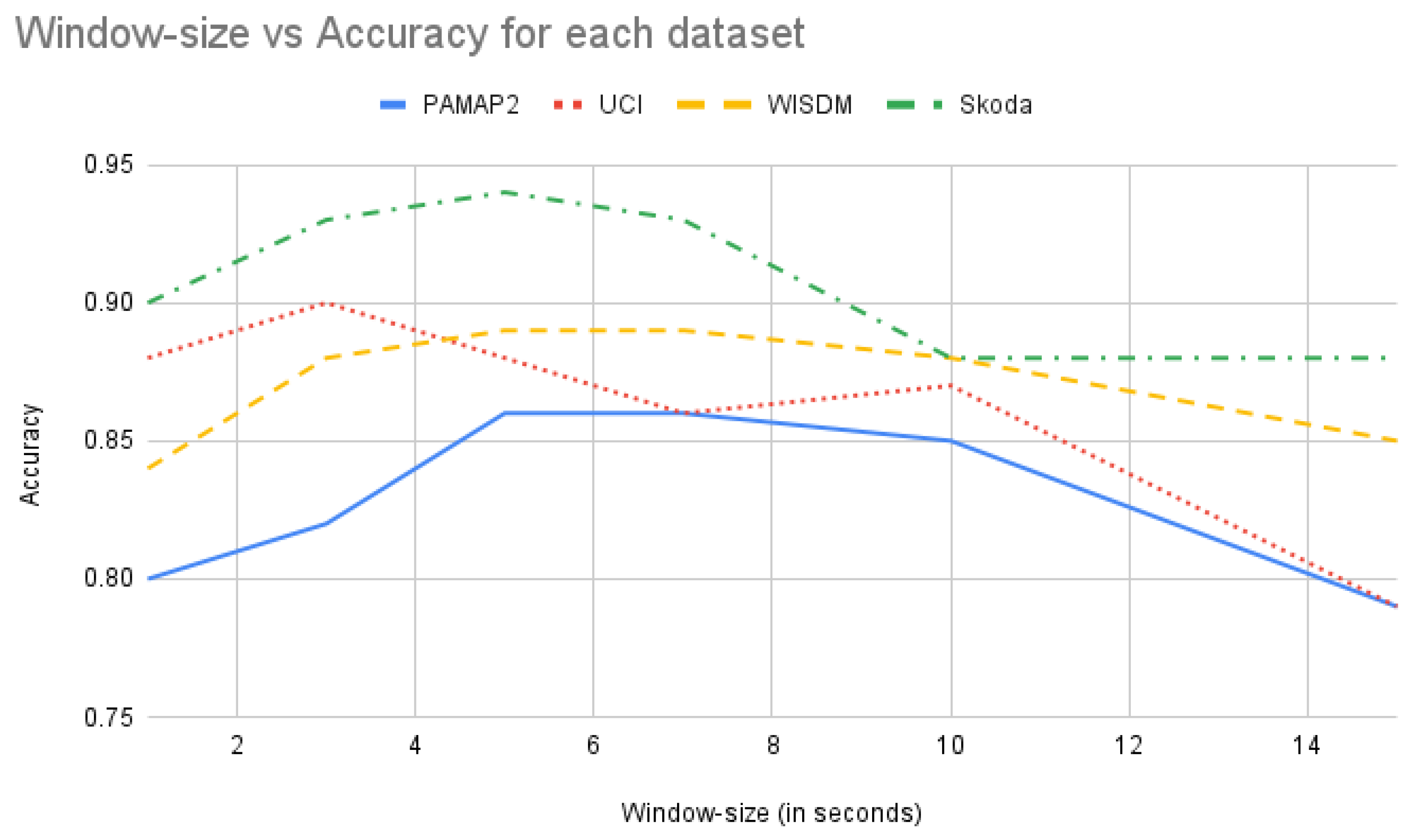
4.6. Window-Size Selection
DTE needs a set of window sizes as input from which the temporal matrices are extracted for model training. In standard HAR the window size is usually chosen empirically for each dataset by experimenting with different values. The previous works provides us with the optimal window size for each of the datasets. In this work as well for each of the datasets, and a standard baseline neural network architecture, the accuracy of action recognition task is plotted with respect to different window sizes (in Figure 11).
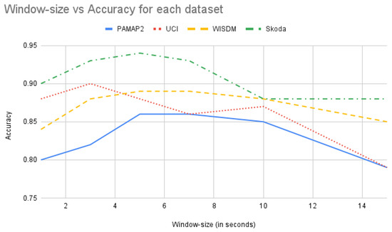
Figure 11.
Accuracy (along y-axis) versus window size (in seconds along x-axis) using the best standard baseline architecture for all the datasets.
This graph provides with an idea of the optimal window size for obtaining best performance for each workload and serves as a empirical foundation in selecting right window sizes for DTE. For construction of the input ensembles with different window sizes the following strategy is adopted: An equal number of values in both directions with uniform stepping from a chosen optimal window-size value. In the PAMAP2 dataset the window size used in [30] is 5.12 s. From Figure 11 similar inferences can be drawn, i.e., the best accuracies are obtained around the 5 s window and 7 s window. It is also observed that for PAMAP2 dataset the accuracy starts improving from 3 s and it starts declining from 10 s, and after 14 s it drops below 0.8. Couple of window-size sets are created between 3 s till 12 s, and the classification matrices of DTE on those sets are tested, e.g., considering 5 s as an optimal time segment, and uniformly stepping on both sides of 5 s, a time-window set (of size 5) can be constructed with [3, 4, 5, 6, 7] s. In a similar manner, different window size sets are created with a different optimal time segment as mid point. These window-size sets are used for training different DTE models and for each window-size set the performance is observed. The results can be seen in Table 5.
Table 5.
HAR accuracy on different set of window sizes using DTE on the datasets using the best architectures (DTE-LSTM on PAMAP2, WISDM, DTE-CNN on UCI, and DTE-ConvLSTM on Skoda).
It is seen that for PAMAP2 the best performing window-size set is the one between 3 s to 7 s. Hence, in the final model this set is used for training. Similar experiments are conducted for the other datasets to obtain the best window sizes for temporal matrix extraction. From the experiments we observed that for Skoda and UCI datasets, the stepping from an optimal window size of 0.5 s is more suitable. Furthermore, for these two datasets lower window sizes are better (can be seen in Figure 11).
5. Future Work
While there are certain caveats and possible future works that could be associated with DTE, they can serve possible direction for future research. One central assumption of DTE is that the trained multiple models are strong learners. If a weak learner exists in the ensemble, it would negatively impact the overall classification and calibration performance. At this point, the window sizes for temporal sequence extraction are empirically chosen to ensure that the learners are strong. An interesting future direction to explore is an automatic adaptive selection of strong learners in the ensemble for DTE. Another downside of having an ensemble is the computational complexity that arises through training multiple models. Distillation of ensembles is a good direction to explore in this context [41]. These caveats expose some exciting research areas that could further improve the domain of reliable HAR. An interesting future direction would be to apply DTE on video-frame-based human activity recognition. The nature of the workload being time-series, DTE could be applied on video frames as well. The most popular architectures for video-based action recognition are spatio-temporal and 3D convolutions [42,43]. It could be promising to test the method on the architectural choices to deliver action recognition from videos. The present version of DTE is focused towards providing well-calibrated predictions. For which it uses a ensemble of models to deliver the inferences. In resource constrained environments where real-time inference is expected (e.g., live predictions using mobile or edge devices), the ensembles might overuse the resource and increase prediction latency. Thus a possible direction to explore is to provide calibrated response through lightweight modeling. Distillation of ensemble models [41] could be an interesting avenue to explore in this regards.
6. Conclusions
This work presents a novel way to incorporate the notion of confidence-calibrated predictions in human activity recognition with wearable sensors. The calibrated predictions representing the actual probability at outputs guarantees reliable modeling that can be safely incorporated into production pipelines, thus enabling safe, sustainable, and improved ubiquitous computing. While addressing the calibration problem, it is also made sure that the primary downstream task of HAR models, i.e., classification, is not hampered in any way.
The devised method called deep time ensembles can applied on any neural network architectures for HAR with sensor data. With a set of different window sizes, temporal matrices are extracted from raw sensor data. These temporal matrices are used to train individual models that are ensembled through an averaging procedure. Combining multiple expert models of the ensemble helps to calibrate the confidence of the softmax distribution and boost the classification measures.
To the best of our knowledge, no previous works have approached calibrating the predictive output of HAR. The approach is validated through extensive experiments on four benchmark datasets of activity recognition from different domains. Our calibration experiments show that in all the datasets, deep time ensembles outperform the calibration measures compared to the baseline models. Our classification experiments demonstrate that DTE boosts the classification performance for almost all the datasets. Thus, the promise of confidence calibrated reliable, as well as improved predictive performance, is delivered through DTE. To demonstrate the ability of the method in calibration, it is also compared with temperature scaling, a popular calibration method for deep learning [14]. Furthermore, our extensive experiments with a variety of DL architectures and datasets can also be used as a guideline for architecture selection in HAR. DTE will open a new research direction of calibrating HAR models as it demonstrates an easy way to obtain reliable confidence measures on wearable time-series input for HAR tasks.
Author Contributions
D.R. conceptualized and conceived the presented idea. D.R. also formulated the theory, performed majority of the experiments, and wrote the manuscript. S.S. investigated the impact of temperature scaling and contributed by performing some experiments. He also contributed in writing-related works, and the Appendix section. S.G. supervised the whole project, and contributed with valuable insights in the Introduction and Methods section. He also contributed to the Abstract and Introduction section of the manuscript. All authors have read and agreed to the published version of the manuscript.
Funding
This project has received funding from the European Union’s Horizon 2020 research and innovation programme under the Marie Skłodowska-Curie grant agreement No 813162. The content of this paper reflects the views only of their author (s). The European Commission/Research Executive Agency are not responsible for any use that may be made of the information it contains.
Institutional Review Board Statement
Not applicable.
Informed Consent Statement
Not applicable.
Data Availability Statement
Not applicable.
Acknowledgments
We would like to acknowledge the effort of Vangjush Komini towards formalizing the Methods section. We would also like to acknowledge the effort of Mohammed El-Beltagy for providing valuable suggestions.
Conflicts of Interest
The authors declare no conflict of interest. The funders had no role in the design of the study; in the collection, analyses, or interpretation of data; in the writing of the manuscript, or in the decision to publish the results.
Abbreviations
The following abbreviations are used in this manuscript:
| AR | Activity Recognition |
| HAR | Human Activity Recognition |
| DTE | Deep Time Ensembles |
| CNN | Convolutional Neural Networks |
| LSTM | Long Short Term Memory |
| ECE | Expected Calibration Error |
Appendix A. Details of Implementation
The implementational details of each model are presented in this section. This is provided to assist in replicating our experiments and results.
Table A1.
PAMAP2 DTE-CNN model configuration.
Table A1.
PAMAP2 DTE-CNN model configuration.
| Category | Configuration |
|---|---|
| Window-sizes (s) | [5, 6, 7, 8, 9] |
| Batch size | 64 |
| Optimizer | Adam |
| Learning rate | 0.00001 |
| L2 regularization | 0.005 |
| Convolutional layer 1 | filters: 128 filter size: 9 stride: 1 padding: valid activation: ReLU |
| Pooling layer | function: max size: 2 stride: 2 |
| Dropout rate | 0.1 |
| Convolutional layer 2 | filters: 128 filter size: 5 stride: 1 padding: valid activation: ReLU |
| Pooling layer | function: max size: 2 stride: 2 |
| Dropout rate | 0.25 |
| Flatten and Dense layers | neurons: 512 activation: ReLU weight reg: L2 |
| Dropout rate | 0.5 |
| Fully connected layer | neurons: number of classes activation: Softmax |
Table A2.
PAMAP2 DTE-LSTM model configuration.
Table A2.
PAMAP2 DTE-LSTM model configuration.
| Category | Configuration |
|---|---|
| Window-sizes (s) | [5, 6, 7, 8, 9] |
| Batch size | 64 |
| Optimizer | Adam |
| Learning rate | 0.001 |
| Dropout rate (before LSTM and Dense layers) | 0.5 |
| 2 LSTM layers | neurons: 256 |
| Fully connected layer | neurons: number of classes activation: Softmax |
Table A3.
UCI DTE CNN model configuration.
Table A3.
UCI DTE CNN model configuration.
| Category | Configuration |
|---|---|
| Window sizes (s) | [1.5, 2, 2.5, 3, 3.5] |
| Batch size | 200 |
| Optimizer | Adam |
| Learning rate | 0.0005 |
| L2 regularization | 0.0005 |
| Dropout rate | 0.25 |
| Convolutional layer | filters: 196 filter size: 16 stride: 1 padding: valid activation: ReLU bias init: 0.01 kernel init: TruncNorm(stddev = 0.01) |
| Pooling layer | function: max size: 4 |
| Fully connected layer | neurons: 1024 activation: Softmax bias init: 0.01 weight init: TruncNorm(stddev = 0.01) kernel reg: L2 |
Table A4.
UCI DTE LSTM model configuration.
Table A4.
UCI DTE LSTM model configuration.
| Category | Configuration |
|---|---|
| Windows sizes | [1.5, 2, 2.5, 3, 3.5] |
| Batch size | 200 |
| Optimizer | Adam |
| Learning rate | 0.001 |
| LSTM layer 1 | neurons: 128 |
| LSTM layer 2 | neurons: 128 return sequence: True |
| Fully connected layer | neurons: number of classes activation: Softmax |
Table A5.
WISDM DTE CNN model configuration.
Table A5.
WISDM DTE CNN model configuration.
| Category | Configuration |
|---|---|
| Window sizes (s) | [6, 7, 8, 9, 10] |
| Batch size | 200 |
| Optimizer | Adam |
| Learning rate | 0.0005 |
| L2 regularization | 0.0005 |
| Dropout rate | 0.25 |
| Convolutional layer | filters: 196 filter size: 16 stride: 1 padding: valid activation: ReLU bias init: 0.01 kernel init: TruncNorm(stddev = 0.01) |
| Pooling layer | function: max size: 4 |
| Fully connected layer | neurons: 1024 activation: Softmax bias init: 0.01 weight init: TruncNorm(stddev = 0.01) kernel reg: L2 |
Table A6.
WISDM DTE LSTM model configuration.
Table A6.
WISDM DTE LSTM model configuration.
| Category | Configuration |
|---|---|
| Window sizes (s) | [6, 7, 8, 9, 10] |
| Batch size | 64 |
| Optimizer | Adam |
| Learning rate | 0.0025 |
| Learning loss rate | 0.0015 |
| 2 LSTM layers | neurons: 30 bias init: 1 |
| Fully connected layer | neurons: number of classes activation: Softmax |
Table A7.
SKODA DTE ConvLSTM model configuration.
Table A7.
SKODA DTE ConvLSTM model configuration.
| Parameter | Configuration |
|---|---|
| Window sizes (s) | [4, 4.5, 5, 5.5, 6] |
| Batch size | 100 |
| Optimizer | RMSProp |
| Learning rate | 0.001 |
| Decay | 0.9 |
| Dropout rate (before LSTM and Dense layers) | 0.5 |
| 3 Convolutional layers | filters: 64 filter size: 5 activation: ReLU |
| 2 LSTM layers | SKODA DTE ConvLSTM model configurationneurons: 128 |
| Fully connected layer | neurons: number of classes activation: Softmax |
Appendix B. Calibration Results
In this section we present the calibration results for datasets and architectures not presented in the main paper. The reliability diagrams demonstrate the calibration improvements by applying DTE to the remaining combinations of models and datasets.
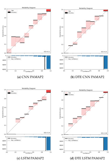
Figure A1.
Reliability diagram of PAMAP2 for (a) CNN, (b) DTE CNN, (c) LSTM, and (d) DTE LSTM.
Figure A1.
Reliability diagram of PAMAP2 for (a) CNN, (b) DTE CNN, (c) LSTM, and (d) DTE LSTM.
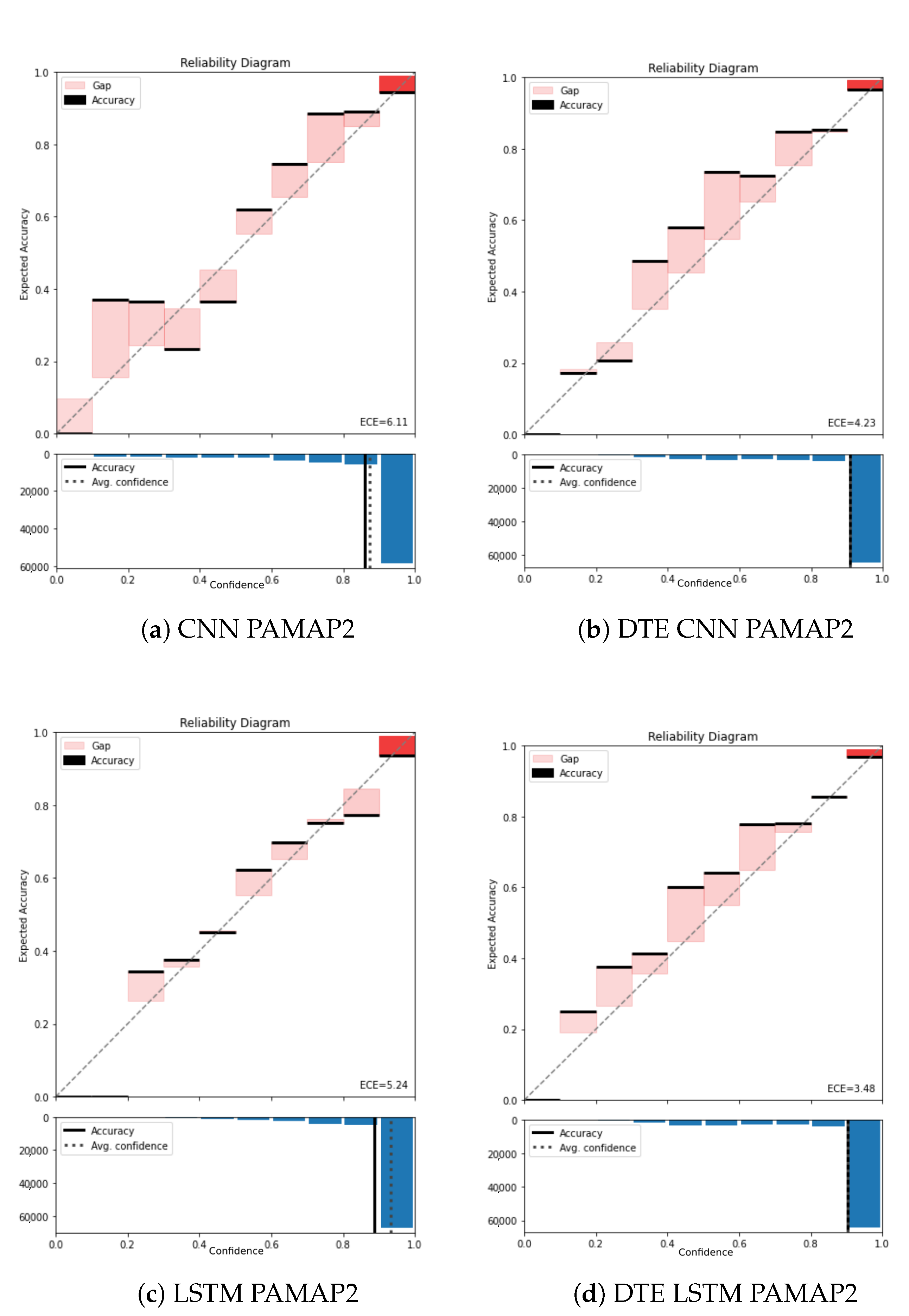
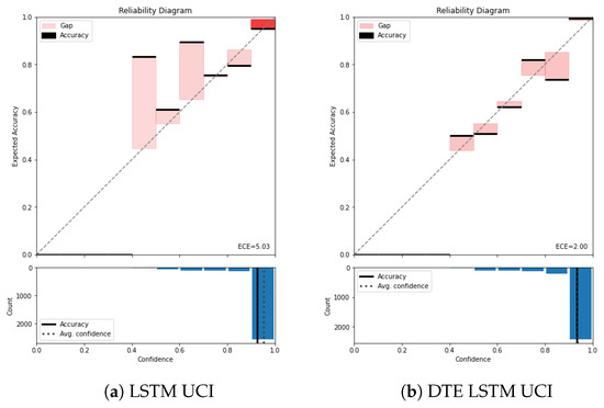
Figure A2.
Reliability diagram of UCI for (a) LSTM and (b) DTE LSTM.
Figure A2.
Reliability diagram of UCI for (a) LSTM and (b) DTE LSTM.


Figure A3.
Reliability diagram of Skoda for (a) ConvLSTM and (b) DTE ConvLSTM.
Figure A3.
Reliability diagram of Skoda for (a) ConvLSTM and (b) DTE ConvLSTM.
Appendix B.1. Calibration Results with Temperature Scaling
In this section, we show the reliability diagrams of PAMAP2 dataset before and after temperature scaling for both CNN and LSTM architecture. As stated before, we initialized the hyperparameter T = 1.5 and tuned it using a validation set in order to smooth the softmax of the baseline models and improve their calibration. For the CNN architecture, the temperature scaling with T = 1.5 worsens the overall calibration (see Figure A4). We observe that in both cases (with and without DTE) the highest bins becomes better calibrated with temperature scaling. Thus, in this scenario TS calibrates the bins where most examples are concentrated at the cost of miscalibrating the lower bins. Furthermore since DTE assigns more examples to the lower bins due to the averaging process, the miscalibration of the lower bins become more pronounced in case of DTE CNN resulting in the highest ECE of 6.10.
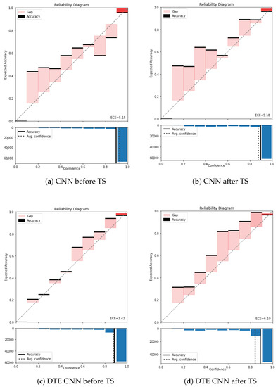
Figure A4.
Reliability diagram of PAMAP2 with and without temperature scaling for CNN and DTE CNN.
Figure A4.
Reliability diagram of PAMAP2 with and without temperature scaling for CNN and DTE CNN.

The model that improved considerably after temperature scaling was the LSTM model trained using PAMAP2 dataset. As shown in Figure A5a,b ECE improved from 5.12% to 3.67%. The DTE is calibrated in itself in this case as well and exhibits more calibration error with temperature scaling.
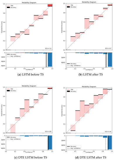
Figure A5.
Reliability diagram of PAMAP2 with and without temperature scaling for LSTM and DTE LSTM.
Figure A5.
Reliability diagram of PAMAP2 with and without temperature scaling for LSTM and DTE LSTM.
We draw attention to the fact that the reliability diagrams for this section was adopted from one of the many experiments repeated towards robustness. Hence, the values of ECE might slightly differ from what we see in the Evaluation section of the paper.
Appendix B.2. Classification Results
In this section we present the confusion matrices of all the classification results that we obtained through our experiments (except the ones already presented). For UCI dataset the confusion matrix is given in Figure A6.
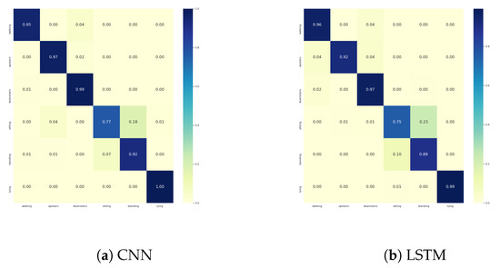
Figure A6.
Confusion matrices of UCI with (a) CNN and (b) LSTM architectures.
Figure A6.
Confusion matrices of UCI with (a) CNN and (b) LSTM architectures.
For PAMAP2 dataset the confusion matrix is given in Figure A7.
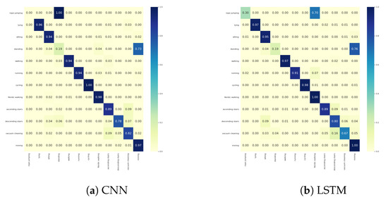
Figure A7.
Confusion matrices of PAMAP2 with (a) CNN and (b) LSTM architectures.
Figure A7.
Confusion matrices of PAMAP2 with (a) CNN and (b) LSTM architectures.
The confusion matrix for WISDM and Skoda dataset for LSTM and Conv LSTM architecture respectively is given in Figure A8.
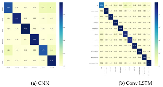
Figure A8.
Confusion matrices of (a) WISDM CNN and (b) Skoda Conv LSTM classification.
Figure A8.
Confusion matrices of (a) WISDM CNN and (b) Skoda Conv LSTM classification.
Appendix C. Number of Ensemble Models
In this section the graph in Figure A9 provides an intuition of the number of ensemble models that are required for DTE. As seen for most of the workloads increasing the size of the ensemble has almost no effect on the accuracy of the F1 score. Hence, for the current setting it is better to stick to a lesser number of models as it will lead to faster inference.
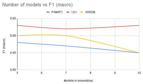
Figure A9.
Number of models (along x-axis) versus F1 (macro) (along y-axis) using.
Figure A9.
Number of models (along x-axis) versus F1 (macro) (along y-axis) using.
References
- Rassem, A.; El-Beltagy, M.; Saleh, M. Cross-country skiing gears classification using deep learning. arXiv 2017, arXiv:1706.08924. [Google Scholar]
- Avci, A.; Bosch, S.; Marin-Perianu, M.; Marin-Perianu, R.; Havinga, P. Activity recognition using inertial sensing for healthcare, wellbeing and sports applications: A survey. In Proceedings of the 23th International Conference on Architecture of Computing Systems 2010, VDE, Hannover, Germany, 22–23 February 2010; pp. 1–10. [Google Scholar]
- Zhang, M.; Sawchuk, A.A. USC-HAD: A daily activity dataset for ubiquitous activity recognition using wearable sensors. In Proceedings of the 2012 ACM Conference on Ubiquitous Computing, Pittsburgh, PA, USA, 5–8 September 2012; pp. 1036–1043. [Google Scholar]
- Hong, Y.J.; Kim, I.J.; Ahn, S.C.; Kim, H.G. Activity recognition using wearable sensors for elder care. In Proceedings of the 2008 Second International Conference on Future Generation Communication and Networking, Hainan, China, 13–15 December 2008; Volume 2, pp. 302–305. [Google Scholar]
- Gal, Y.; Ghahramani, Z. Dropout as a bayesian approximation: Representing model uncertainty in deep learning. In Proceedings of the International Conference on Machine Learning, New York, NY, USA, 20–22 June 2016; pp. 1050–1059. [Google Scholar]
- Guan, Y.; Plötz, T. Ensembles of deep lstm learners for activity recognition using wearables. ACM Interact. Mob. Wearable Ubiquitous Technol. 2017, 1, 1–28. [Google Scholar] [CrossRef] [Green Version]
- Kumar, A.; Liang, P.; Ma, T. Verified uncertainty calibration. arXiv 2019, arXiv:1909.10155. [Google Scholar]
- Dietterich, T.G. Ensemble methods in machine learning. In Lecture Notes in Computer Science, Proceedings of the International Workshop on Multiple Classifier Systems, Cagliari, Italy, 21–23 June 2000; Springer: Berlin/Heidelberg, Germany, 2000; pp. 1–15. [Google Scholar]
- Seo, S.; Seo, P.H.; Han, B. Learning for single-shot confidence calibration in deep neural networks through stochastic inferences. In Proceedings of the IEEE/CVF Conference on Computer Vision and Pattern Recognition, Long Beach, CA, USA, 16–20 June 2019; pp. 9030–9038. [Google Scholar]
- Weiss, G.M.; Yoneda, K.; Hayajneh, T. Smartphone and smartwatch-based biometrics using activities of daily living. IEEE Access 2019, 7, 133190–133202. [Google Scholar] [CrossRef]
- Anguita, D.; Ghio, A.; Oneto, L.; Parra, X.; Reyes-Ortiz, J.L. A public domain dataset for human activity recognition using smartphones. Esann 2013, 3, 3. [Google Scholar]
- Reiss, A.; Stricker, D. Introducing a new benchmarked dataset for activity monitoring. In Proceedings of the 2012 16th International Symposium on Wearable Computers, Newcastle, UK, 18–22 June 2012; pp. 108–109. [Google Scholar]
- Stiefmeier, T.; Roggen, D.; Ogris, G.; Lukowicz, P.; Tröster, G. Wearable activity tracking in car manufacturing. IEEE Pervasive Comput. 2008, 7, 42–50. [Google Scholar] [CrossRef]
- Guo, C.; Pleiss, G.; Sun, Y.; Weinberger, K.Q. On calibration of modern neural networks. In Proceedings of the International Conference on Machine Learning, PMLR, Sydney, Australia, 6–11 August 2017; pp. 1321–1330. [Google Scholar]
- Bao, L.; Intille, S.S. Activity recognition from user-annotated acceleration data. In Lecture Notes in Computer Science, Proceedings of the International Conference on Pervasive Computing, Linz/Vienna, Austria, 21–23 April 2004; Springer: Berlin/Heidelberg, Germany, 2004; pp. 1–17. [Google Scholar]
- Casale, P.; Pujol, O.; Radeva, P. Human activity recognition from accelerometer data using a wearable device. In Lecture Notes in Computer Science, Proceedings of the Iberian Conference on Pattern Recognition and Image Analysis, Las Palmas de Gran Canaria, Spain, 8–10 June 2011; Springer: Berlin/Heidelberg, Germany, 2011; pp. 289–296. [Google Scholar]
- Feng, Z.; Mo, L.; Li, M. A Random Forest-based ensemble method for activity recognition. In Proceedings of the 2015 37th Annual International Conference of the IEEE Engineering in Medicine and Biology Society (EMBC), Milan, Italy, 25–29 August 2015; pp. 5074–5077. [Google Scholar]
- He, Z.; Jin, L. Activity recognition from acceleration data based on discrete consine transform and SVM. In Proceedings of the 2009 IEEE International Conference on Systems, Man and Cybernetics, San Antonio, TX, USA, 11–14 October 2009; pp. 5041–5044. [Google Scholar]
- He, Z.Y.; Jin, L.W. Activity recognition from acceleration data using AR model representation and SVM. In Proceedings of the 2008 International Conference on Machine Learning and Cybernetics, Kunming, China, 12–15 July 2008; Volume 4, pp. 2245–2250. [Google Scholar]
- Ignatov, A. Real-time human activity recognition from accelerometer data using Convolutional Neural Networks. Appl. Soft Comput. 2018, 62, 915–922. [Google Scholar] [CrossRef]
- Ordóñez, F.J.; Roggen, D. Deep convolutional and lstm recurrent neural networks for multimodal wearable activity recognition. Sensors 2016, 16, 115. [Google Scholar] [CrossRef] [PubMed] [Green Version]
- Yao, S.; Hu, S.; Zhao, Y.; Zhang, A.; Abdelzaher, T. Deepsense: A unified deep learning framework for time-series mobile sensing data processing. In Proceedings of the 26th International Conference on World Wide Web, Perth, Australia, 3–7 April 2017; pp. 351–360. [Google Scholar]
- Ishimaru, S.; Hoshika, K.; Kunze, K.; Kise, K.; Dengel, A. Towards reading trackers in the wild: Detecting reading activities by EOG glasses and deep neural networks. In Proceedings of the 2017 ACM International Joint Conference on Pervasive and Ubiquitous Computing and Proceedings of the 2017 ACM International Symposium on Wearable Computers, Maui, HI, USA, 11–15 September 2017; pp. 704–711. [Google Scholar]
- Jiang, W.; Yin, Z. Human activity recognition using wearable sensors by deep convolutional neural networks. In Proceedings of the 23rd ACM International Conference on Multimedia, Brisbane, Australia, 26–30 October 2015; pp. 1307–1310. [Google Scholar]
- Lecun, Y.; Bottou, L.; Bengio, Y.; Haffner, P. Gradient-based learning applied to document recognition. Proc. IEEE 1998, 86, 2278–2324. [Google Scholar] [CrossRef] [Green Version]
- Hochreiter, S.; Schmidhuber, J. Long Short-Term Memory. Neural Comput. 1997, 9, 1735–1780. [Google Scholar] [CrossRef] [PubMed]
- Murad, A.; Pyun, J.Y. Deep recurrent neural networks for human activity recognition. Sensors 2017, 17, 2556. [Google Scholar] [CrossRef] [PubMed] [Green Version]
- Wang, L. Recognition of human activities using continuous autoencoders with wearable sensors. Sensors 2016, 16, 189. [Google Scholar] [CrossRef] [PubMed]
- Agarwal, P.; Alam, M. A lightweight deep learning model for human activity recognition on edge devices. Procedia Comput. Sci. 2020, 167, 2364–2373. [Google Scholar] [CrossRef]
- Hammerla, N.Y.; Halloran, S.; Plötz, T. Deep, convolutional, and recurrent models for human activity recognition using wearables. arXiv 2016, arXiv:1604.08880. [Google Scholar]
- Platt, J. Probabilistic outputs for support vector machines and comparisons to regularized likelihood methods. Adv. Large Margin Classif. 1999, 10, 61–74. [Google Scholar]
- Zadrozny, B.; Elkan, C. Obtaining calibrated probability estimates from decision trees and naive bayesian classifiers. ICML Citeseer 2001, 1, 609–616. [Google Scholar]
- Zadrozny, B.; Elkan, C. Transforming classifier scores into accurate multiclass probability estimates. In Proceedings of the Eighth ACM SIGKDD International Conference on Knowledge Discovery and Data Mining, Edmonton, AB, Canada, 23–26 July 2002; pp. 694–699. [Google Scholar]
- Naeini, M.P.; Cooper, G.; Hauskrecht, M. Obtaining well calibrated probabilities using bayesian binning. In Proceedings of the AAAI Conference on Artificial Intelligence, Austin, TX, USA, 25–30 January 2015; Volume 29. [Google Scholar]
- Lakshminarayanan, B.; Pritzel, A.; Blundell, C. Simple and scalable predictive uncertainty estimation using deep ensembles. In Proceedings of the Advances in Neural Information Processing Systems, Long Beach, CA, USA, 4–9 December 2017; pp. 6402–6413. [Google Scholar]
- Song, Y.; Viventi, J.; Wang, Y. Diversity encouraged learning of unsupervised LSTM ensemble for neural activity video prediction. arXiv 2016, arXiv:1611.04899. [Google Scholar]
- Beluch, W.H.; Genewein, T.; Nürnberger, A.; Köhler, J.M. The power of ensembles for active learning in image classification. In Proceedings of the IEEE Conference on Computer Vision and Pattern Recognition, Salt Lake City, UT, USA, 18–22 June 2018; pp. 9368–9377. [Google Scholar]
- DeGroot, M.H.; Fienberg, S.E. The comparison and evaluation of forecasters. J. R. Stat. Soc. Ser. D (The Stat.) 1983, 32, 12–22. [Google Scholar] [CrossRef]
- Reliability Diagrams. Available online: https://github.com/hollance/reliability-diagrams (accessed on 30 April 2021).
- Naftaly, U.; Intrator, N.; Horn, D. Optimal ensemble averaging of neural networks. Netw. Comput. Neural Syst. 1997, 8, 283–296. [Google Scholar] [CrossRef] [Green Version]
- Malinin, A.; Mlodozeniec, B.; Gales, M. Ensemble distribution distillation. arXiv 2019, arXiv:1905.00076. [Google Scholar]
- Tran, D.; Bourdev, L.; Fergus, R.; Torresani, L.; Paluri, M. Learning spatiotemporal features with 3d convolutional networks. In Proceedings of the IEEE International Conference on Computer Vision, Santiago, Chile, 11–18 December 2015; pp. 4489–4497. [Google Scholar]
- Tran, D.; Wang, H.; Torresani, L.; Ray, J.; LeCun, Y.; Paluri, M. A closer look at spatiotemporal convolutions for action recognition. In Proceedings of the IEEE Conference on Computer Vision and Pattern Recognition, Salt Lake City, UT, USA, 18–22 June 2018; pp. 6450–6459. [Google Scholar]


Publisher’s Note: MDPI stays neutral with regard to jurisdictional claims in published maps and institutional affiliations. |
© 2021 by the authors. Licensee MDPI, Basel, Switzerland. This article is an open access article distributed under the terms and conditions of the Creative Commons Attribution (CC BY) license (https://creativecommons.org/licenses/by/4.0/).