
Estimation of Mechanical Power Output Employing Deep Learning on Inertial Measurement Data in Roller Ski Skating

 ,
, 
 ,
,
Abstract
:1. Introduction
2. Material and Methods
2.1. Participants
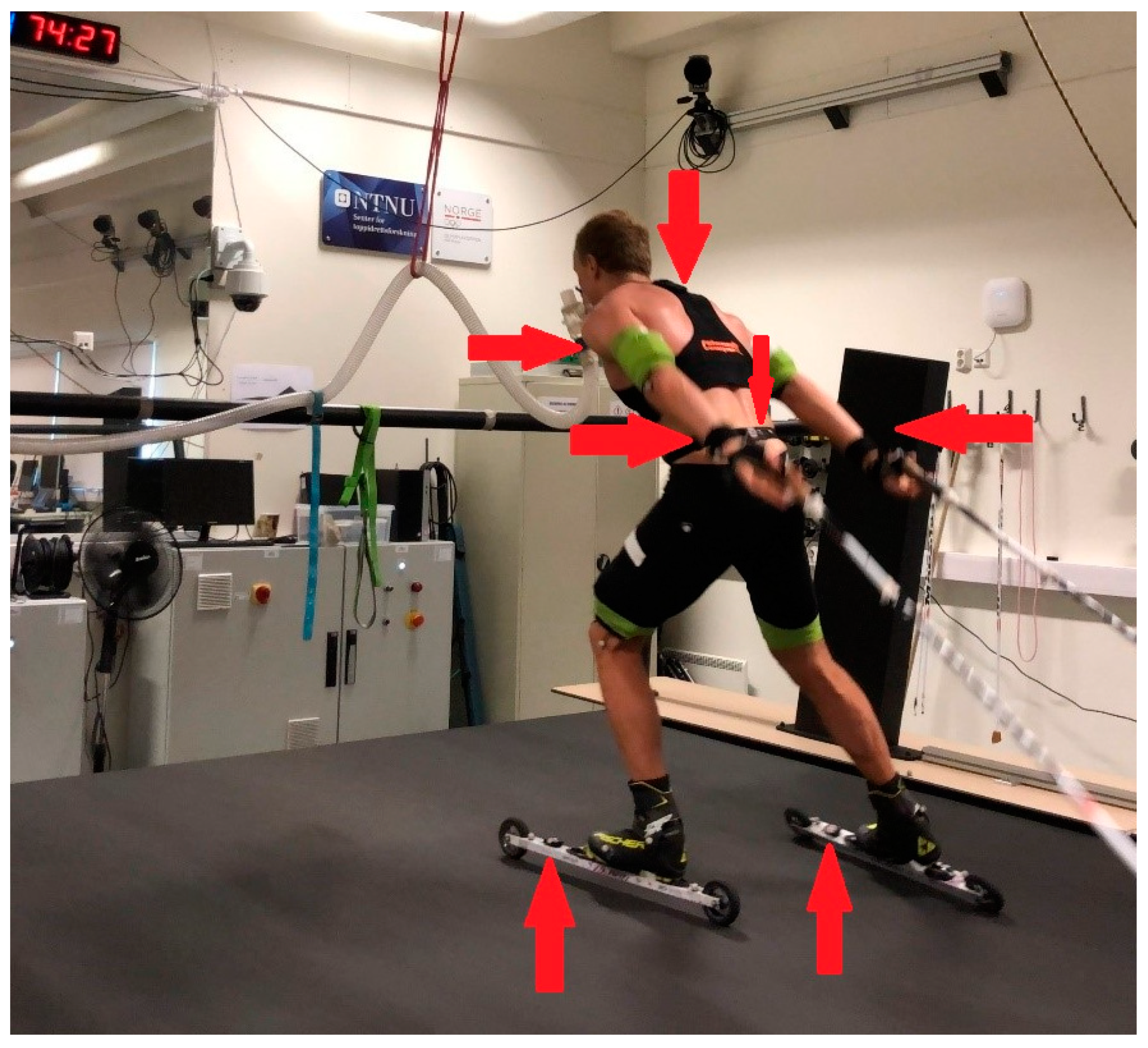
2.2. Equipment
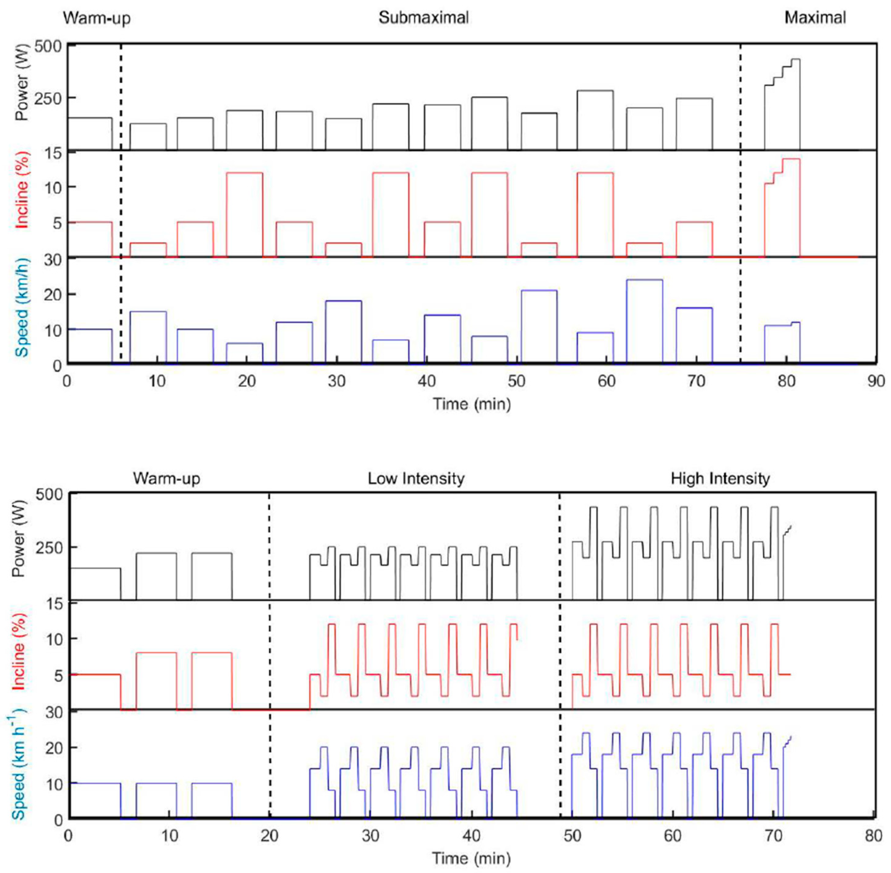
2.3. Test Protocol
2.4. Data Processing
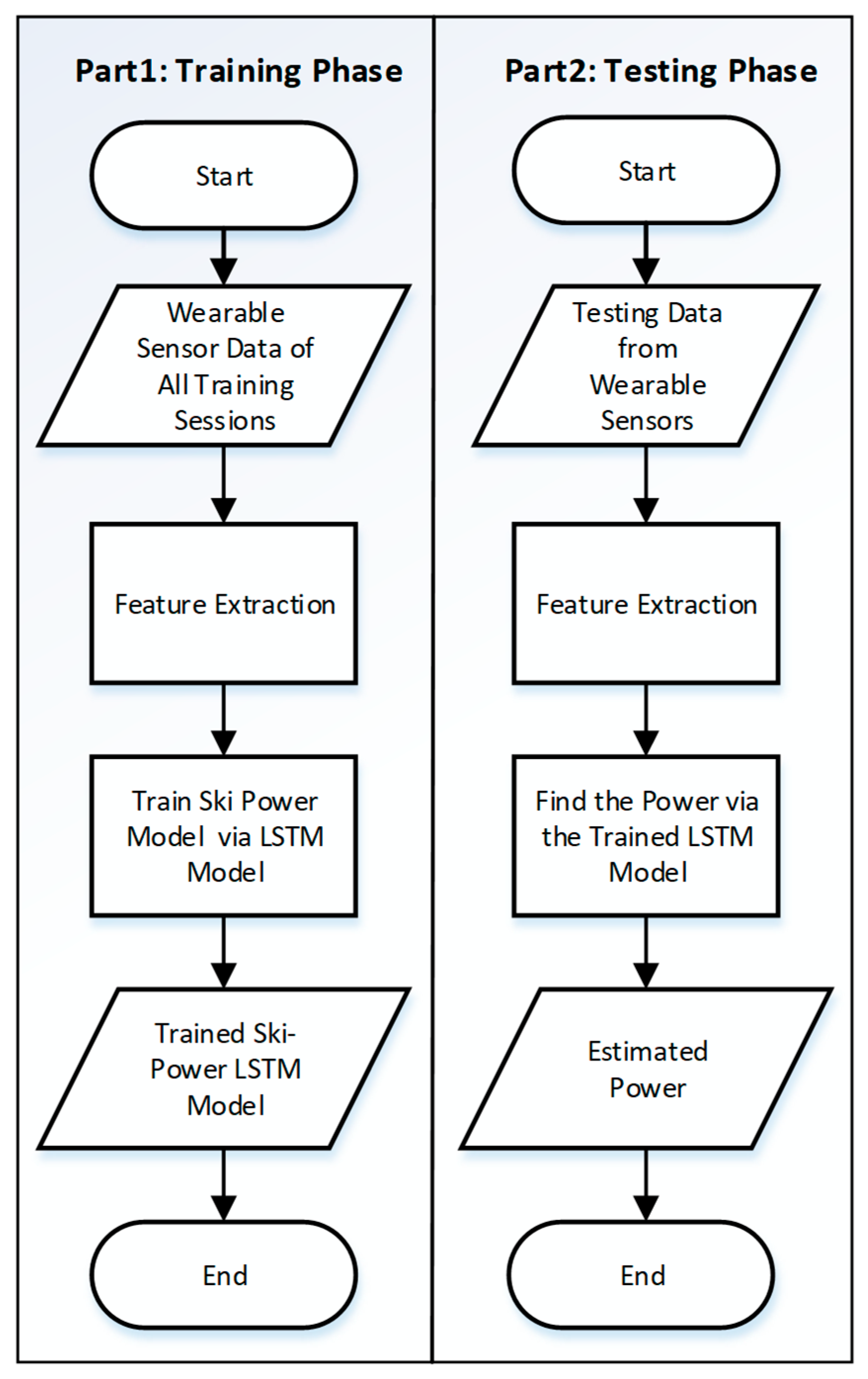
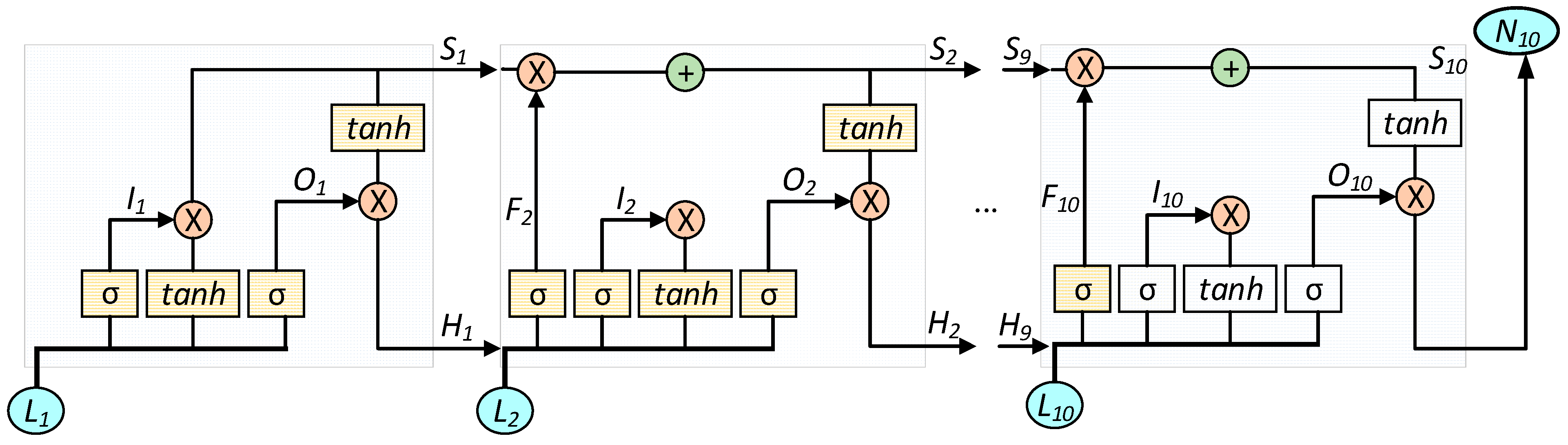
2.5. Machine Learning Model
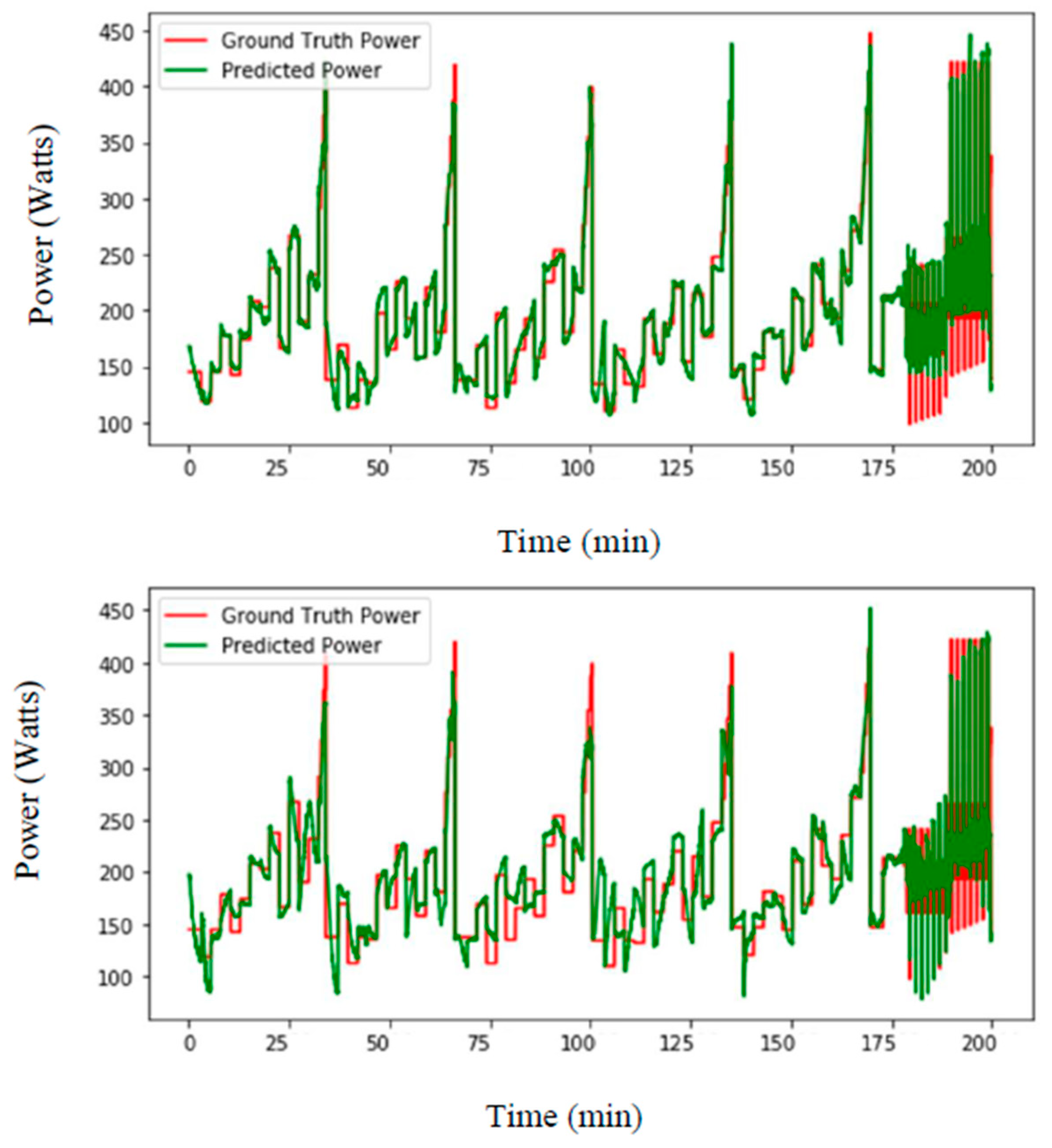
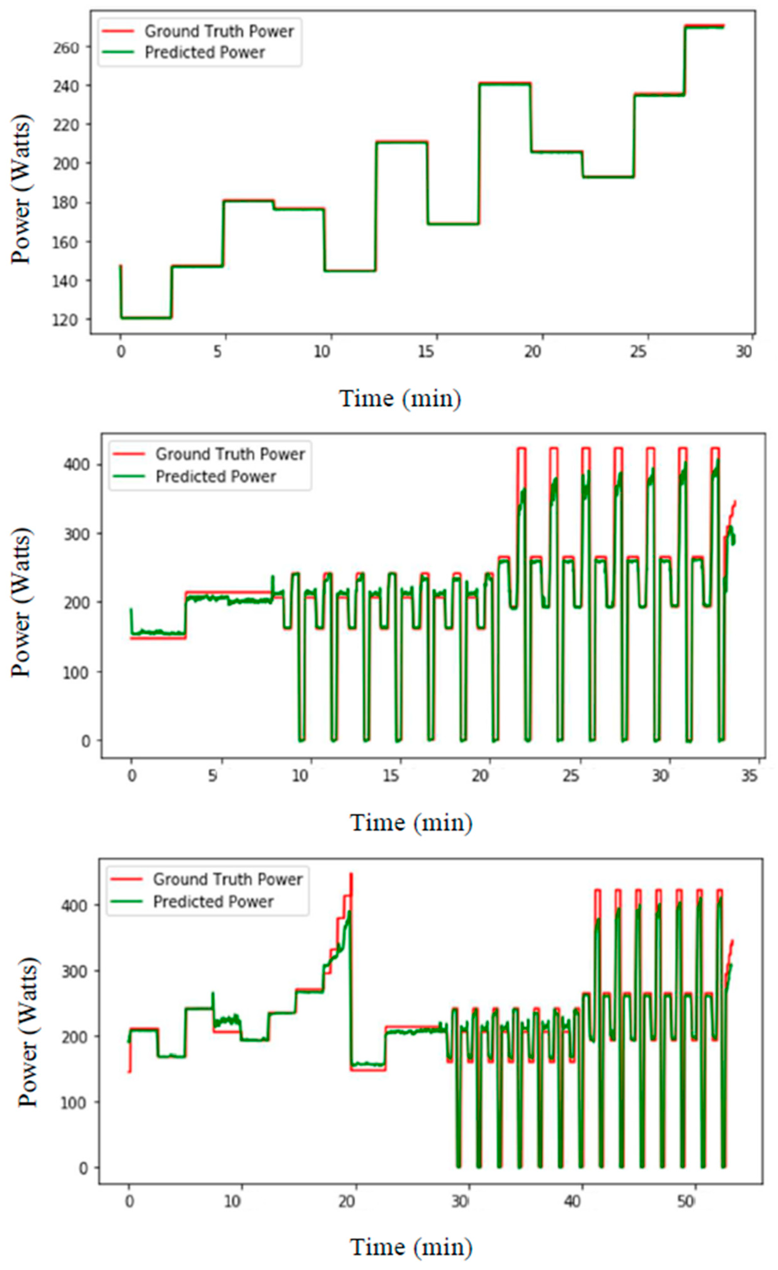
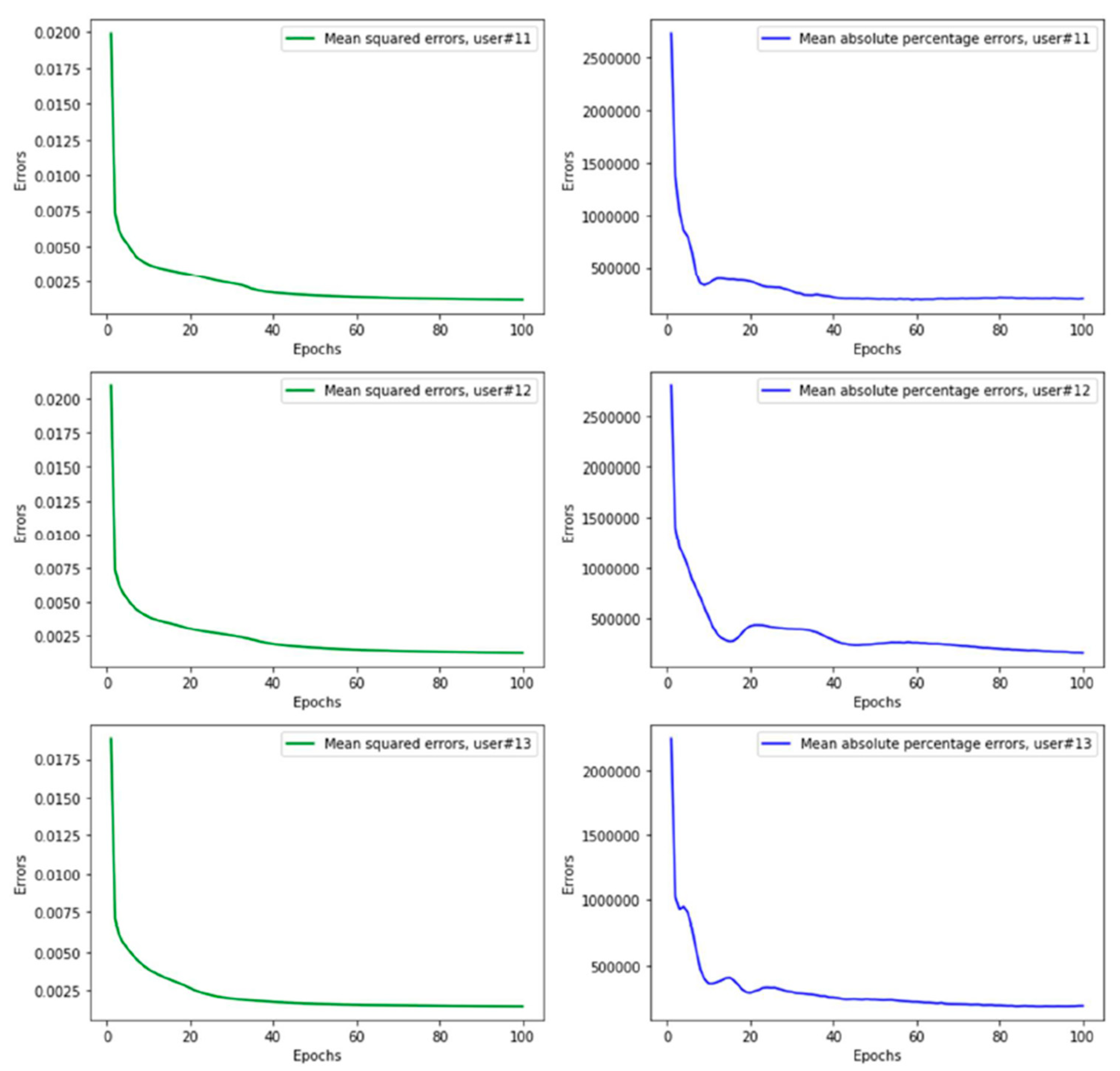
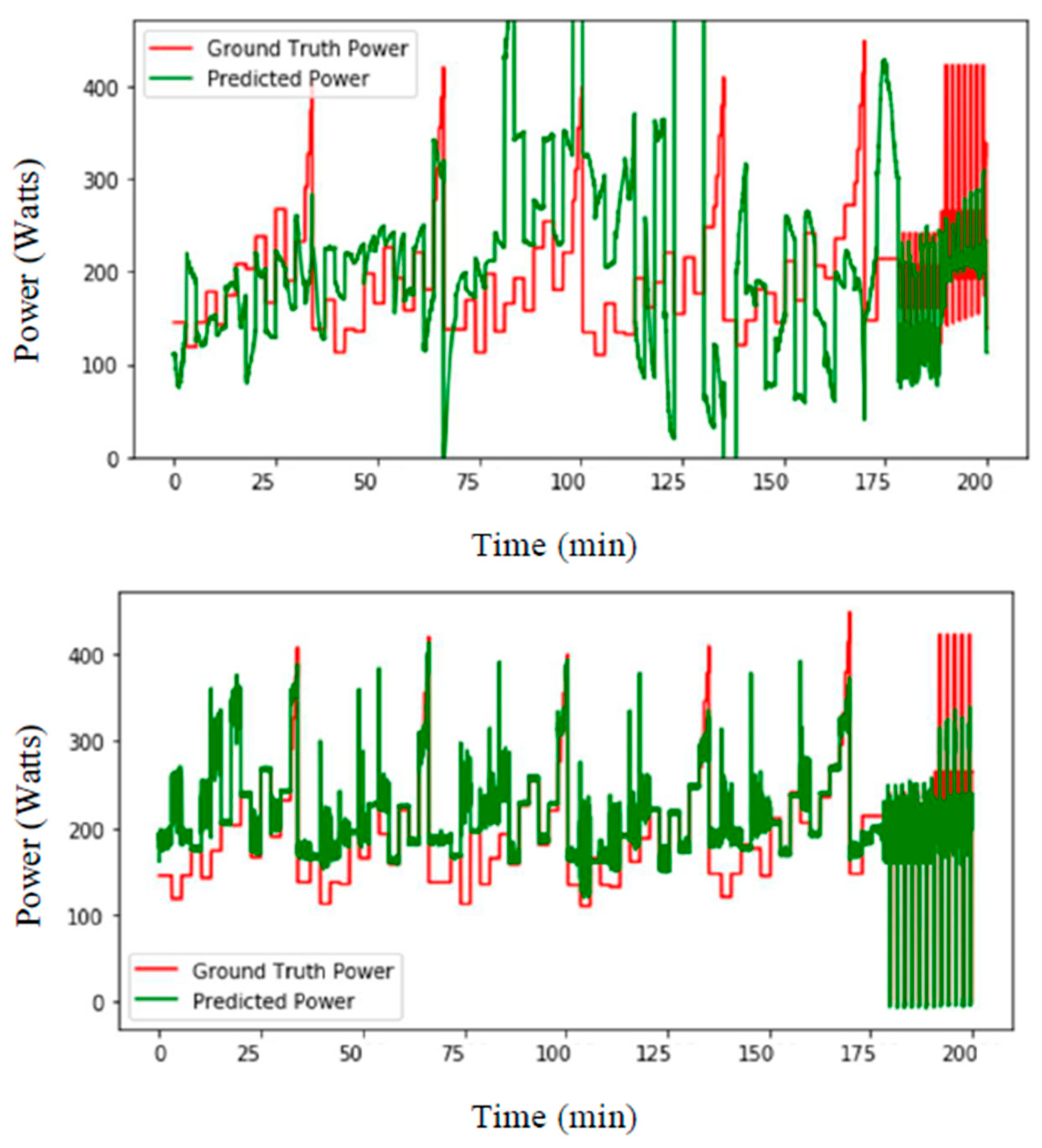
3. Experimental Setups and Results
4. Discussion
5. Conclusions
Author Contributions
Funding
Institutional Review Board Statement
Informed Consent Statement
Data Availability Statement
Acknowledgments
Conflicts of Interest
References
- Sandbakk, Ø.; Holmberg, H.C. Physiological capacity and training routines of elite cross-country skiers: Approaching the upper limits of human endurance. Int. J. Sports Physiol. Perform. 2017, 12, 1003–1011. [Google Scholar] [CrossRef] [PubMed]
- Sandbakk, Ø.; Ettema, G.; Holmberg, H.C. The influence of incline and speed on work rate, gross efficiency and kinematics of roller ski skating. Eur. J. Appl. Physiol. 2012, 112, 2829–2838. [Google Scholar] [CrossRef] [PubMed]
- Karlsson, Ø.; Gilgien, M.; Gløersen, Ø.N.; Rud, B.; Losnegard, T. Exercise intensity during cross-country skiing described by oxygen demands in flat and uphill terrain. Front. Physiol. 2018, 9, 846. [Google Scholar] [CrossRef]
- Gløersen, Ø.N.; Gilgien, M.; Dysthe, D.K.; Malthe-Sørenssen, A.; Losnegard, T.J. Oxygen demand, uptake, and deficits in elite cross-country skiers during a 15-km race. Med. Sci. Sport. Exerc. 2020, 52, 983–992. [Google Scholar] [CrossRef] [PubMed] [Green Version]
- Saibene, F.; Cortili, G.; Roi, G.; Colombini, A. The energy cost of level cross-country skiing and the effect of the friction of the ski. Eur. J. Appl. Physiol. Occup. Physiol. 1989, 58, 791–795. [Google Scholar] [CrossRef]
- Allen, H.; Coggan, A.R.; McGregor, S. Training and Racing with a Power Meter; VeloPress: Boulder, CO, USA, 2019. [Google Scholar]
- Ohtonen, O.; Lindinger, S.; Lemmettylä, T.; Seppälä, S.; Linnamo, V. Validation of portable 2D force binding systems for cross-country skiing. Sport. Eng. 2013, 16, 281–296. [Google Scholar] [CrossRef]
- Moxnes, J.F.; Sandbakk, O.; Hausken, K. A simulation of cross-country skiing on varying terrain by using a mathematical power balance model. Open Access J. Sport. Med. 2013, 4, 127–139. [Google Scholar]
- Gløersen, Ø.; Losnegard, T.; Malthe-Sørenssen, A.; Dysthe, D.K.; Gilgien, M. Propulsive Power in Cross-Country Skiing: Application and Limitations of a Novel Wearable Sensor-Based Method During Roller Skiing. Front. Physiol. 2018, 9, 1631. [Google Scholar] [CrossRef]
- Imbach, F.; Candau, R.; Chailan, R.; Perrey, S. Validity of the Stryd Power Meter in Measuring Running Parameters at Submaximal Speeds. Sports 2020, 8, 103. [Google Scholar] [CrossRef]
- Cerezuela-Espejo, V.; Hernández-Belmonte, A.; Courel-Ibáñez, J.; Conesa-Ros, E.; Mora-Rodríguez, R.; Pallarés, J.G. Are we ready to measure running power? Repeatability and concurrent validity of five commercial technologies. Eur. J. Sport Sci. 2020, 21, 1–10. [Google Scholar] [CrossRef]
- Jaén-Carrillo, D.; Roche-Seruendo, L.E.; Cartón-Llorente, A.; Ramírez-Campillo, R.; García-Pinillos, F. Mechanical Power in Endurance Running: A Scoping Review on Sensors for Power Output Estimation during Running. Sensors 2020, 20, 6482. [Google Scholar] [CrossRef] [PubMed]
- Fasel, B.; Favre, J.; Chardonnens, J.; Gremion, G.; Aminian, K. An inertial sensor-based system for spatio-temporal analysis in classic cross-country skiing diagonal technique. J. Biomech. 2015, 48, 3199–3205. [Google Scholar] [CrossRef] [PubMed]
- Myklebust, H. Quantification of Movement Patterns in Cross-Country Skiing Using Inertial Measurement Units. Ph.D. Thesis, Norwegian School of Sport Sciences, Oslo, Norway, 2016. [Google Scholar]
- Seeberg, T.M.; Tjønnås, J.; Rindal, O.M.H.; Haugnes, P.; Dalgard, S.; Sandbakk, Ø. A multi-sensor system for automatic analysis of classical cross-country skiing techniques. Sport. Eng. 2017, 20, 313–327. [Google Scholar] [CrossRef]
- Tjønnås, J.; Seeberg, T.M.; Rindal, O.M.H.; Haugnes, P.; Sandbakk, Ø. Assessment of basic motions and technique identification in classical cross-country skiing. Front. Psychol. 2019, 10, 1260. [Google Scholar] [CrossRef] [Green Version]
- Rindal, O.M.H.; Seeberg, T.M.; Tjønnås, J.; Haugnes, P.; Sandbakk, Ø. Automatic classification of sub-techniques in classical cross-country skiing using a machine learning algorithm on micro-sensor data. Sensors 2018, 18, 75. [Google Scholar] [CrossRef] [Green Version]
- Agrawal, A.; Ahuja, R. Deep Learning Algorithms for Human Activity Recognition: A Comparative Analysis BT—Cybernetics, Cognition and Machine Learning Applications; Gunjan, V.K., Suganthan, P.N., Haase, J., Kumar, A., Eds.; Springer: Singapore, 2021; pp. 391–402. [Google Scholar]
- Hinton, G.E.; Osindero, S.; Teh, Y.-W. A fast learning algorithm for deep belief nets. Neural Comput. 2006, 18, 1527–1554. [Google Scholar] [CrossRef]
- Uddin, M.Z.; Khaksar, W.; Torresen, J. Facial expression recognition using salient features and convolutional neural network. IEEE Access 2017, 5, 26146–26161. [Google Scholar] [CrossRef]
- Graves, A.; Mohamed, A.; Hinton, G. Speech recognition with deep recurrent neural networks. In Proceedings of the 2013 IEEE International Conference on Acoustics, Speech and Signal Processing, Vancouver, BC, Canada, 26–31 May 2013; pp. 6645–6649. [Google Scholar]
- Mekruksavanich, S.; Jitpattanakul, A. Lstm networks using smartphone data for sensor-based human activity recognition in smart homes. Sensors 2021, 21, 1636. [Google Scholar] [CrossRef]
- Sherratt, F.; Plummer, A.; Iravani, P. Understanding LSTM network behaviour of IMU-based locomotion mode recognition for applications in prostheses and wearables. Sensors 2021, 21, 1264. [Google Scholar] [CrossRef]
- Yang, Z.; Zheng, X. Hand Gesture Recognition based on Trajectories Features and Computation-Efficient Reused LSTM Network. IEEE Sens. J. 2021, 15, 16945–16960. [Google Scholar] [CrossRef]
- Guang, X.; Gao, Y.; Liu, P.; Li, G. IMU Data and GPS Position Information Direct Fusion Based on LSTM. Sensors 2021, 21, 2500. [Google Scholar] [CrossRef]
- Curreri, F.; Patanè, L.; Xibilia, M.G. RNN-and LSTM-Based Soft Sensors Transferability for an Industrial Process. Sensors 2021, 21, 823. [Google Scholar] [CrossRef]
- Liu, P.; Wang, J.; Guo, Z. Multiple and complete stability of recurrent neural networks with sinusoidal activation function. IEEE Trans. Neural Netw. Learn. Syst. 2020, 32, 229–240. [Google Scholar] [CrossRef] [PubMed]
- Seeberg, T.M.; Kocbach, J.; Danielsen, J.; Noordhof, D.A.; Skovereng, K.; Haugnes, P.; Tjønnås, J.; Sandbakk, Ø. Physiological and Biomechanical Determinants of Sprint Ability Following Variable Intensity Exercise When Roller Ski Skating. Front. Physiol. 2021, 12, 384. [Google Scholar] [CrossRef] [PubMed]
- Sandbakk, Ø.; Holmberg, H.C.; Leirdal, S.; Ettema, G. Metabolic rate and gross efficiency at high work rates in world class and national level sprint skiers. Eur. J. Appl. Physiol. 2010, 109, 473–481. [Google Scholar] [CrossRef] [PubMed]
- International Ski Federation. The International Ski Competition Rules (ICR), Book II: Cross-Country; International Ski Federation: Oberhofen, Switzerland, 2020. [Google Scholar]
- Chen, Z. An LSTM Recurrent Network for Step Counting. arXiv 2018, arXiv:1802.03486. [Google Scholar]


| User-Dependent Data Included in Training | Body Mass not Included | Body Mass Included | ||
|---|---|---|---|---|
| MSE (W) | RE (%) | MSE (W) | RE (%) | |
| 10% | 11.5 | 3.8 | 10.9 | 3.5 |
| 5% | 14.1 | 5.0 | 13.7 | 4.9 |
| 1% | 27.0 | 10.0 | 24.6 | 8.9 |
| 0.5% | 36.5 | 14.3 | 34.1 | 12.9 |
| 0% | 144.4 | 50.9 | 57.2 | 17.9 |
| LSTM | CNN | ANN | |||||||
|---|---|---|---|---|---|---|---|---|---|
| Age (year) | Height (cm) | Mass (kg) | MSE (W) | RE (%) | MSE (W) | RE (%) | MSE (W) | RE (%) | |
| Subject 1 | 28 | 186.5 | 83.1 | 35.8 | 9.4 | 49.9 | 13.1 | 49.3 | 12.9 |
| Subject 2 | 21 | 180 | 73.1 | 54.0 | 14.3 | 64.3 | 17.0 | 62.3 | 16.5 |
| Subject 3 | 25 | 194.5 | 84.6 | 58.0 | 12.6 | 62.9 | 13.6 | 62.9 | 13.6 |
| Subject 4 | 24 | 190.5 | 81.1 | 55.9 | 12.5 | 61.2 | 13.7 | 62.0 | 13.9 |
| Subject 5 | 29 | 181 | 78.5 | 49.6 | 17.4 | 49.7 | 17.4 | 50.3 | 17.6 |
| Subject 6 | 28 | 185 | 77.5 | 48.6 | 18.5 | 56.8 | 21.6 | 51.5 | 19.6 |
| Subject 7 | 22 | 180.1 | 83.5 | 56.4 | 18.5 | 58.5 | 19.2 | 57.6 | 18.9 |
| Subject 8 | 27 | 196.5 | 91.6 | 57.6 | 16.7 | 60.4 | 17.5 | 60.9 | 17.6 |
| Subject 9 | 26 | 180.5 | 78.1 | 20.3 | 4.7 | 62.9 | 14.5 | 61.9 | 14.3 |
| Subject 10 | 21 | 181 | 74.1 | 26.2 | 5.3 | 30.2 | 6.1 | 27.4 | 5.5 |
| Subject 11 | 23 | 183.5 | 74 | 21.7 | 4.5 | 24.9 | 5.1 | 24.8 | 5.1 |
| Subject 12 | 22 | 176.5 | 72.1 | 33.1 | 8.5 | 33.6 | 8.7 | 34.0 | 8.8 |
| Subject 13 | 26 | 177 | 79.3 | 30.3 | 7.5 | 31.7 | 7.9 | 33.9 | 8.4 |
| Mean | 24.8 | 184.0 | 79.28 | 42.1 | 11.6 | 49.8 | 13.5 | 49.1 | 13.3 |
| SD | 2.8 | 6.3 | 5.52 | 14.5 | 5.3 | 14.5 | 5.2 | 14.2 | 4.9 |
Publisher’s Note: MDPI stays neutral with regard to jurisdictional claims in published maps and institutional affiliations. |
© 2021 by the authors. Licensee MDPI, Basel, Switzerland. This article is an open access article distributed under the terms and conditions of the Creative Commons Attribution (CC BY) license (https://creativecommons.org/licenses/by/4.0/).
Share and Cite
Uddin, M.Z.; Seeberg, T.M.; Kocbach, J.; Liverud, A.E.; Gonzalez, V.; Sandbakk, Ø.; Meyer, F. Estimation of Mechanical Power Output Employing Deep Learning on Inertial Measurement Data in Roller Ski Skating. Sensors 2021, 21, 6500. https://doi.org/10.3390/s21196500
Uddin MZ, Seeberg TM, Kocbach J, Liverud AE, Gonzalez V, Sandbakk Ø, Meyer F. Estimation of Mechanical Power Output Employing Deep Learning on Inertial Measurement Data in Roller Ski Skating. Sensors. 2021; 21(19):6500. https://doi.org/10.3390/s21196500
Chicago/Turabian StyleUddin, Md Zia, Trine M. Seeberg, Jan Kocbach, Anders E. Liverud, Victor Gonzalez, Øyvind Sandbakk, and Frédéric Meyer. 2021. "Estimation of Mechanical Power Output Employing Deep Learning on Inertial Measurement Data in Roller Ski Skating" Sensors 21, no. 19: 6500. https://doi.org/10.3390/s21196500
APA StyleUddin, M. Z., Seeberg, T. M., Kocbach, J., Liverud, A. E., Gonzalez, V., Sandbakk, Ø., & Meyer, F. (2021). Estimation of Mechanical Power Output Employing Deep Learning on Inertial Measurement Data in Roller Ski Skating. Sensors, 21(19), 6500. https://doi.org/10.3390/s21196500