
Low-Power Failure Detection for Environmental Monitoring Based on IoT


Abstract
:1. Introduction
- We have designed a novel FD for environmental monitoring based on the IoT that ensures a high availability, and a reliable execution, of applications.
- The detection period can be calculated by the reliability function of the Weibull distribution, and it has a proportional relationship to the reliability of the sensors.
- Due to the variable detection period, the number of communications per unit time is reduced, which saves on sensor power consumption and detection overhead.
2. Related Work
2.1. Environmental Monitoring of IoT
2.2. Failure Detection
2.3. QoS Metrics of Failure Detection
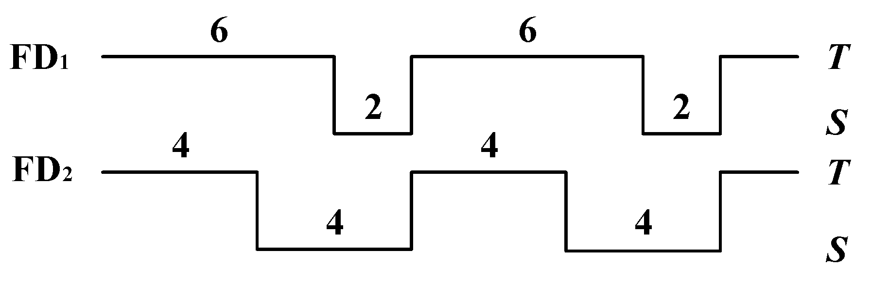
- Detection time () is from the moment a node crashes to the moment it is permanently suspected, i.e., when the final S-transition occurs.
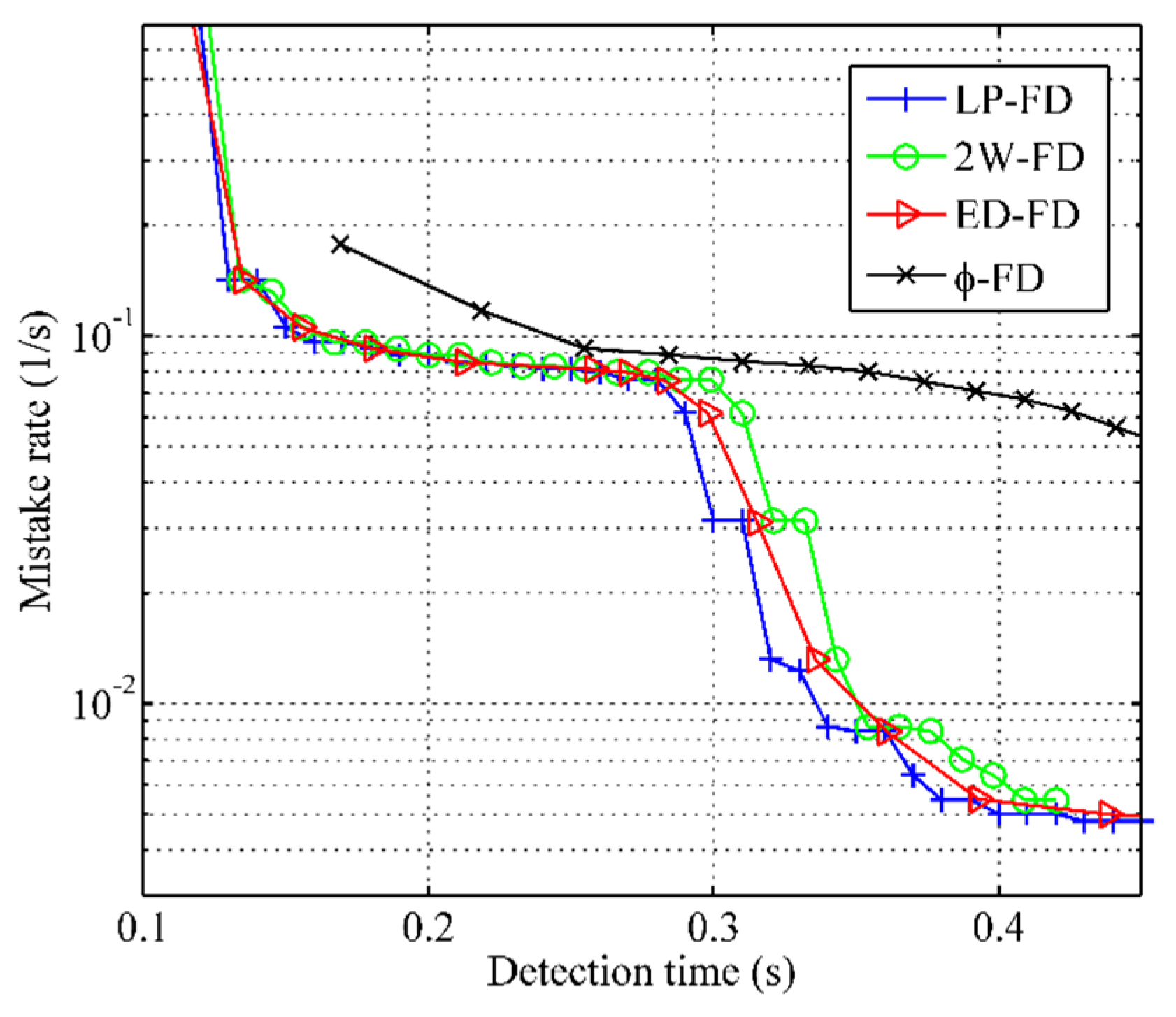
- Mistake rate () is the number of false suspicions a failure detector makes per unit time, i.e., it is used to describe the frequency of false suspicions of a failure detector.
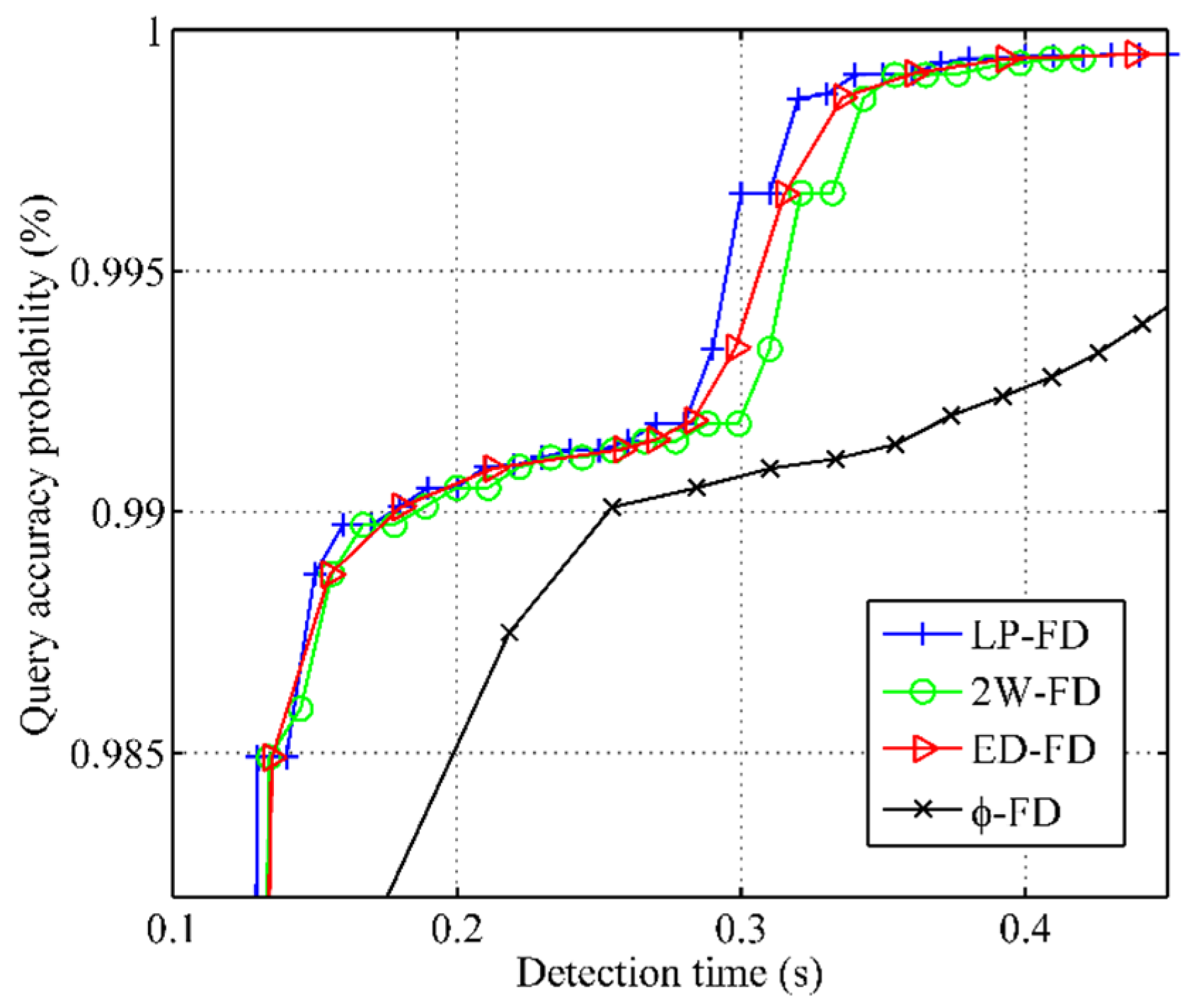
- Query accuracy probability () is the probability that the output of a failure detector is correct at a random time.
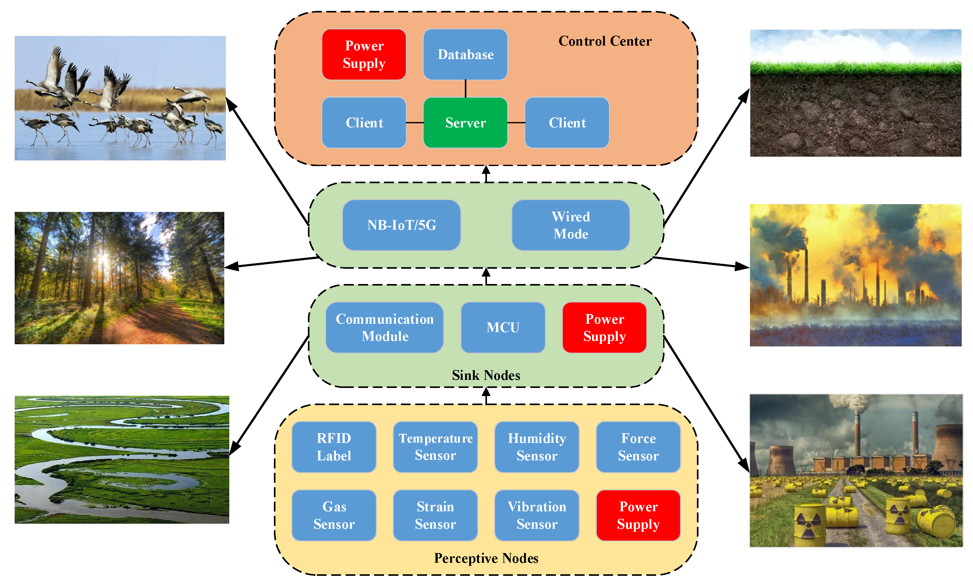
3. Proposed System
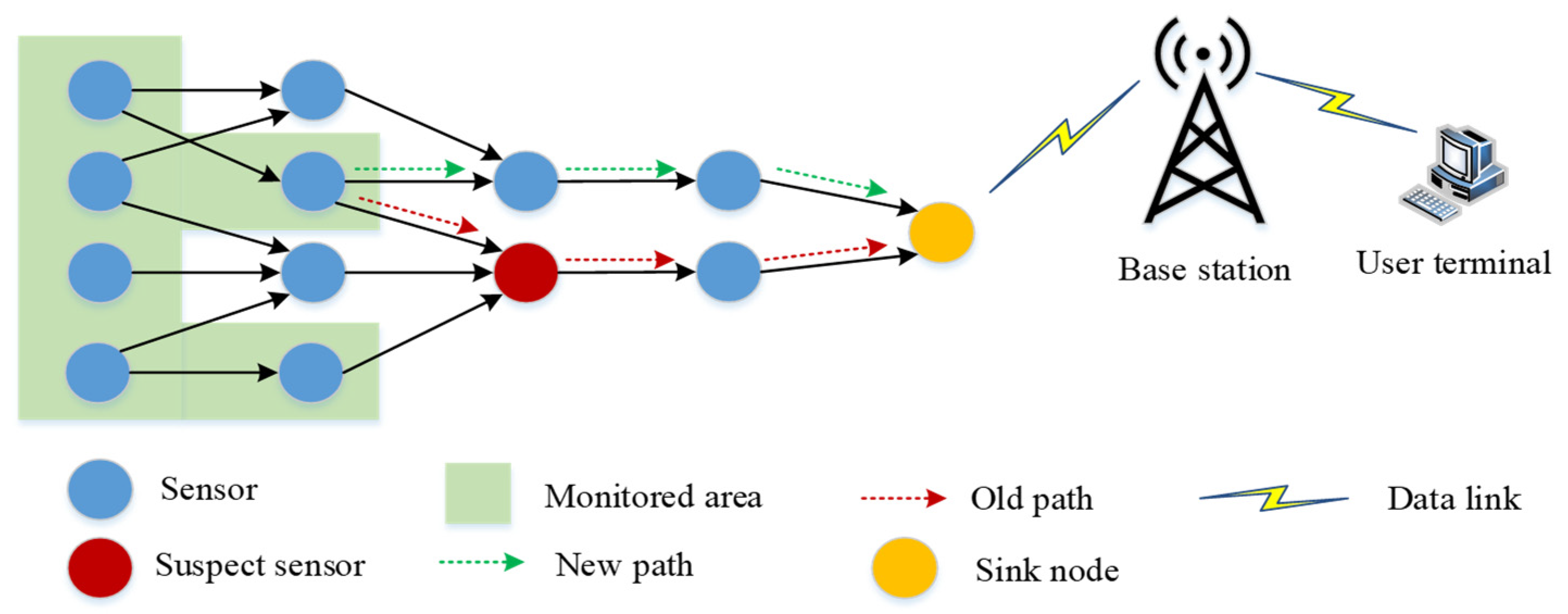
3.1. Network Model
3.2. Link Failure
3.3. Node Failure
4. Implementation of Low-Power Failure Detector
4.1. The Detection Period
| Algorithm 1. Detection Period. |
| Input: , , , , |
| Output: |
| 1. |
| 2. if |
| 3. then ; |
| 4. ; |
| 5. if (n>1) |
| 6. then ; |
| 7. else if |
| 8. then ; |
| 9. else |
| 10. ; |
| 11. end if |
| 12. end if |
| 13. else |
| 14. ; |
| 15. end if |
4.2. Implementation of Low-Power Failure Detector
| Algorithm 2. Low-power Failure Detector. |
| Input: , |
| Output: suspectlist[] |
| 1. Node q: /*monitoring node*/ |
| 2. Task 1: |
| 3. if and did not receive heartbeat within freshpoint |
| 4. then add p to suspectlist[]; |
| 5. end if |
| 6. Task 2: |
| 7. upon receiving heartbeat message from p; |
| 8. if |
| 9. if |
| 10. then remove p from suspectlist[]; |
| 11. ; |
| 12. else |
| 13. ; |
| 14. end if |
| 15. ; |
| 16. ; |
| 17. ; |
| 18. ; |
| 19. ; |
| 20. end if |
| 21. Node p: /*detected node*/ |
| 22. for all do |
| 23. at time : (the i-th detection period); |
| 24. send heartbeat message to node q; |
| 25. ; |
| 26. end for |
5. Evaluation and Performance
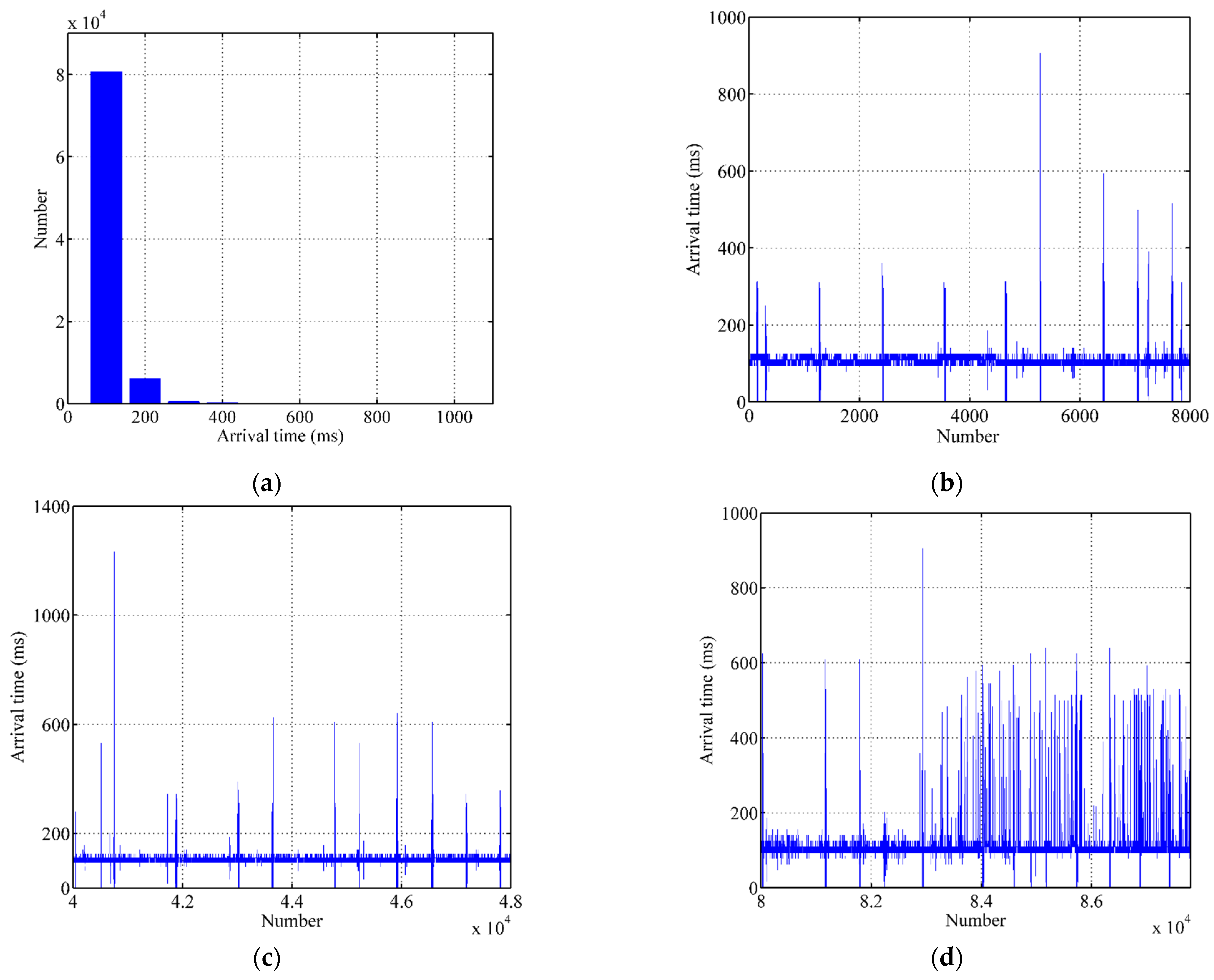
5.1. Data Processing
5.2. Discussions on Parameters
5.3. Comparison of Failure Detection Metrics
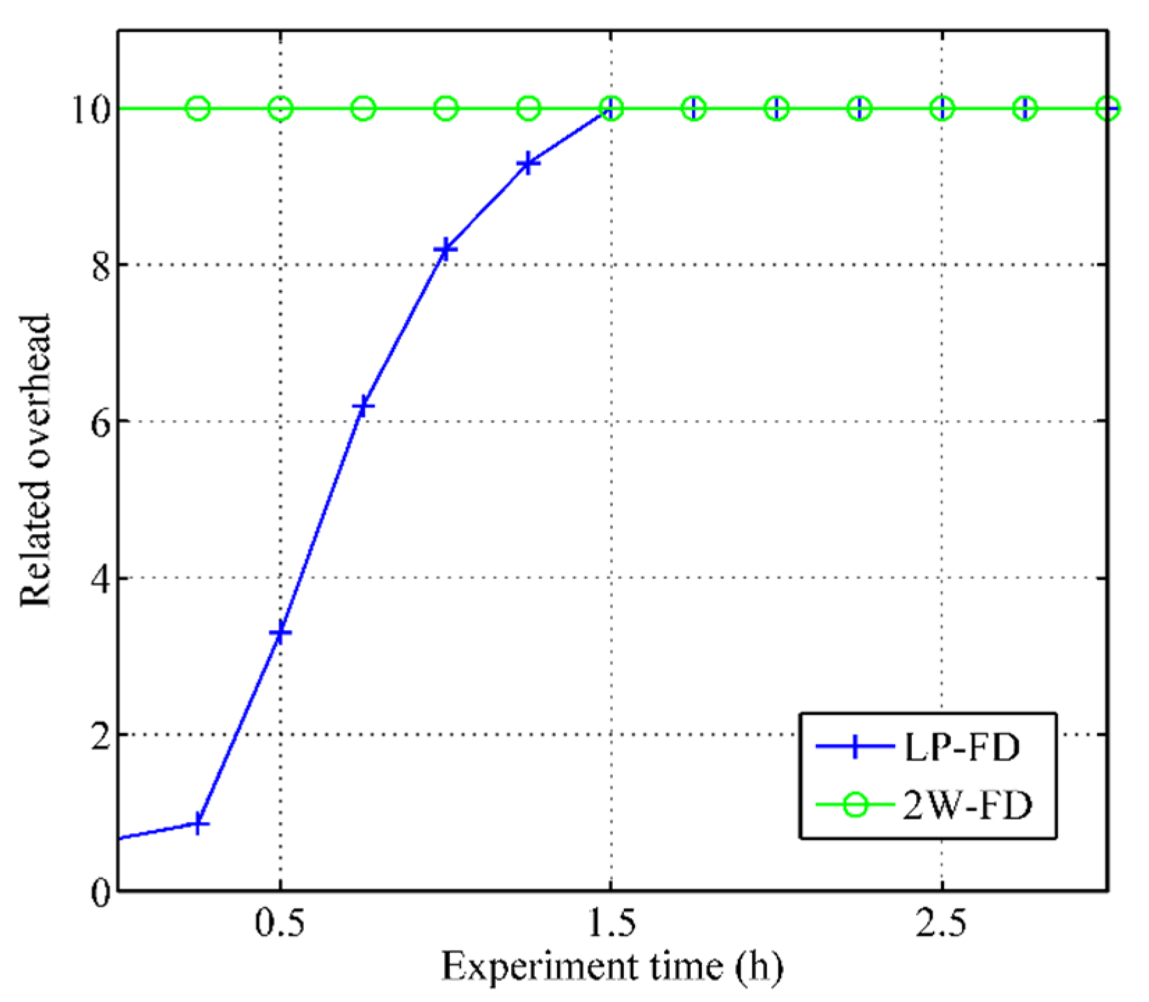
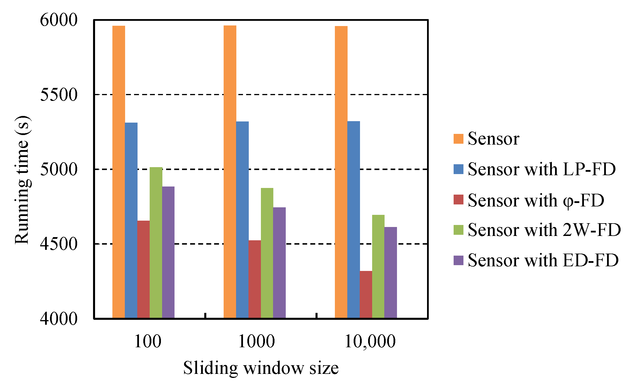
5.4. Comparison of Battery Consumption
6. Conclusions
Author Contributions
Funding
Institutional Review Board Statement
Informed Consent Statement
Conflicts of Interest
References
- Atzori, L.; Iera, A.; Morabito, G. The Internet of Things: A survey. Comput. Netw. 2010, 54, 2787–2805. [Google Scholar] [CrossRef]
- Neshenko, N.; Bou-Harb, E.; Crichigno, J. Demystifying IoT security: An exhaustive survey on IoT vulnerabilities and a first empirical look on Internet-scale IoT exploitations. IEEE Commun. Surv. Tutor. 2019, 21, 2702–2733. [Google Scholar] [CrossRef]
- Domingo, M. An overview of the Internet of underwater things. J. Netw. Comput. Appl. 2012, 35, 1879–1890. [Google Scholar] [CrossRef]
- Shuai, X.; Qian, H. Design of wetland monitoring system based on the Internet of Things. Procedia Environ. Sci. 2011, 11, 1046–1051. [Google Scholar]
- Aa, A.; Rb, B.; Na, C. FaaVPP: Fog as a virtual power plant service for community energy management. Future Gener. Comput. Syst. 2020, 20, 675–683. [Google Scholar]
- Muaafa, M.; Ramirez-Marquez, J. Engineering management models for urban security. IEEE Trans. Eng. Manag. 2017, 64, 29–41. [Google Scholar] [CrossRef]
- Xiong, N.; Athanasios, V.; Jie, W.; Richard, Y.; Yi, P. A self-tuning failure detection scheme for cloud computing service. In Proceedings of the IPDPS, Shanghai, China, 21–25 May 2012; pp. 668–679. [Google Scholar]
- Tomsic, A.; Sens, P.; Garcia, J.; Arantes, L.; Sopena, J. 2W-FD: A failure detector algorithm with QoS. In Proceedings of the IPDPS, Hyderabad, India, 25–29 May 2015; pp. 885–893. [Google Scholar]
- Hayashibara, N.; Defago, X.; Yared, R.; Katayama, T. The φ accrual failure detector. In Proceedings of the SRDS, Florianopolis, Brazil, 18–20 October 2004; pp. 66–78. [Google Scholar]
- Bosilca, G.; Bouteiller, A.; Thomas, G.; Yves, H.; Sens, P.; Dongarra, J. A failure detector for HPC platforms. Int. J. High Perform. Comput. Appl. 2018, 32, 139–158. [Google Scholar] [CrossRef] [Green Version]
- He, Y.; Jiang, X.; Fan, Z. Self-adaptive failure detector for peer-to-peer distributed system considering the link faults. In Proceedings of the APPT, Santiago de Compostela, Spain, 28 August 2017; pp. 64–75. [Google Scholar]
- Turchetti, R.; Duarte, P.; Arantes, L. A QoS congurable failure detection service for Internet applications. J. Internet Serv. Appl. 2016, 7, 1–14. [Google Scholar] [CrossRef] [Green Version]
- Ko, H.; Pack, S.; Leung, V. Spatiotemporal correlation-based environmental monitoring system in energy harvesting Internet of Things (IoT). IEEE Trans. Ind. Inform. 2019, 15, 2958–2968. [Google Scholar] [CrossRef]
- Lu, T.; Chen, X.; Bai, W. Research on environmental monitoring and control technology based on intelligent Internet of Things perception. J. Eng. 2019, 23, 8946–8950. [Google Scholar] [CrossRef]
- Zhu, Z.; Zheng, H.; Ye, P. The research and prospect for hardware system of intelligent control of greenhouse environment. Adv. Mater. Res. 2014, 3227, 69–74. [Google Scholar] [CrossRef]
- Veerle, D.; Anjia, H.; Kumps, M.; Petrovic, C. Circadian variation in post void residual in nursing home residents with moderate impairment in activities of daily living. J. Am. Med. Dir. Assoc. 2016, 11, 433–437. [Google Scholar]
- Bogdan, P.; Duda, A.; Hwang, W.; Theoleyre, F. Efficient topology construction for RPL over IEEE 802.15.4 in wireless sensor networks. Ad. Hoc. Netw. 2013, 8, 25–38. [Google Scholar]
- Liu, Z. Hardware design of smart home system based on ZigBee wireless sensor network. AASRI Procedia 2014, 13, 78–81. [Google Scholar] [CrossRef]
- Peng, Y.; Wang, D. Overview of wireless sensor network localization technology. J. Electr. Measur. Instr. 2011, 5, 389–399. [Google Scholar] [CrossRef]
- Li, J.; Guo, M.; Feng, X. Evaluation system of agricultural IoT development: Reviews and prospects. Res. Agric. M 2016, 37, 423–429. [Google Scholar]
- Zhang, Y.; Liu, X.; Geng, X.; Li, D. IoT forest environmental factors collection platform based on ZigBee. Cybern. Inf. Technol. 2015, 14, 51–62. [Google Scholar]
- Lakshman, A.; Malik, P. Cassandra: A decentralized structured storage system. SIGOPS Oper. Syst. Rev. 2010, 44, 35–40. [Google Scholar] [CrossRef]
- Chen, W.; Toueg, S.; Aguilera, M.K. On the quality of service of failure detectors. IEEE Trans. Comput. 2002, 51, 561–580. [Google Scholar] [CrossRef]
- Xiong, N.; Defago, X. ED FD: Improving the Phi accrual failure detector. JAIST 2007, 1, 1–29. [Google Scholar]
- Felber, P.; Defago, X.; Guerraoui, R.; Oser, P. Failure detectors as first class objects. In Proceedings of the DOA, Edinburgh, UK, 6 September 1999; pp. 132–141. [Google Scholar]
- Ravishankar, R.; Vrudhula, S.; Rakhmatov, D. Battery modeling for energy-Aware system design. Computer 2003, 36, 77–85. [Google Scholar] [CrossRef]
- Xiong, N.; Vasilakos, A.; Yang, T.; Song, L.; Pan, Y.; Kannan, R.; Li, Y. Comparative analysis of quality of service and memory usage for adaptive failure detectors in healthcare systems. IEEE J. Sel. Areas Commun. 2009, 27, 495–509. [Google Scholar] [CrossRef]
- Xiong, N.; Vasilakos, A.; Wei, S.; Yang, Y. General traffic-feature analysis for an effective failure detector in fault-tolerant wired and wireless networks. Tech. Rep. 2011, 1, 1–25. [Google Scholar]
- Khan, I.; Belqasmi, F.; Glitho, R.; Crespi, N.; Morrow, M.; Polakos, P. Wireless sensor network virtualization: A survey. IEEE Commun. Surv. Tutor. 2016, 18, 553–576. [Google Scholar] [CrossRef] [Green Version]
- Bhoi, S.K.; Khilar, P.M. Self Soft Fault Detection based Routing Protocol for Vehicular ad hoc Network in City Environment. Wirel. Netw. 2016, 22, 1–21. [Google Scholar] [CrossRef]


| Symbol | Definition |
|---|---|
| detection period | |
| reliability function of Weibull distribution | |
| scale parameter of Weibull distribution | |
| shape parameter of Weibull distribution | |
| time difference between a certain time and calculated time based on reliability | |
| preset minimum detection period | |
| EA | expected time arrival of next heartbeat message |
| freshpoint of heartbeat message | |
| SM | safety margin |
| predictive heartbeat message delay | |
| d | heartbeat message delay |
| arrival time of new heartbeat message | |
| number of lost heartbeat messages | |
| sequence number of heartbeat messages |
Publisher’s Note: MDPI stays neutral with regard to jurisdictional claims in published maps and institutional affiliations. |
© 2021 by the authors. Licensee MDPI, Basel, Switzerland. This article is an open access article distributed under the terms and conditions of the Creative Commons Attribution (CC BY) license (https://creativecommons.org/licenses/by/4.0/).
Share and Cite
Liu, J.; Gao, W.; Dong, J.; Wu, N.; Ding, F. Low-Power Failure Detection for Environmental Monitoring Based on IoT. Sensors 2021, 21, 6489. https://doi.org/10.3390/s21196489
Liu J, Gao W, Dong J, Wu N, Ding F. Low-Power Failure Detection for Environmental Monitoring Based on IoT. Sensors. 2021; 21(19):6489. https://doi.org/10.3390/s21196489
Chicago/Turabian StyleLiu, Jiaxi, Weizhong Gao, Jian Dong, Na Wu, and Fei Ding. 2021. "Low-Power Failure Detection for Environmental Monitoring Based on IoT" Sensors 21, no. 19: 6489. https://doi.org/10.3390/s21196489
APA StyleLiu, J., Gao, W., Dong, J., Wu, N., & Ding, F. (2021). Low-Power Failure Detection for Environmental Monitoring Based on IoT. Sensors, 21(19), 6489. https://doi.org/10.3390/s21196489