
Enhanced Human Activity Recognition Using Wearable Sensors via a Hybrid Feature Selection Method

Abstract
:1. Introduction
2. Related Works
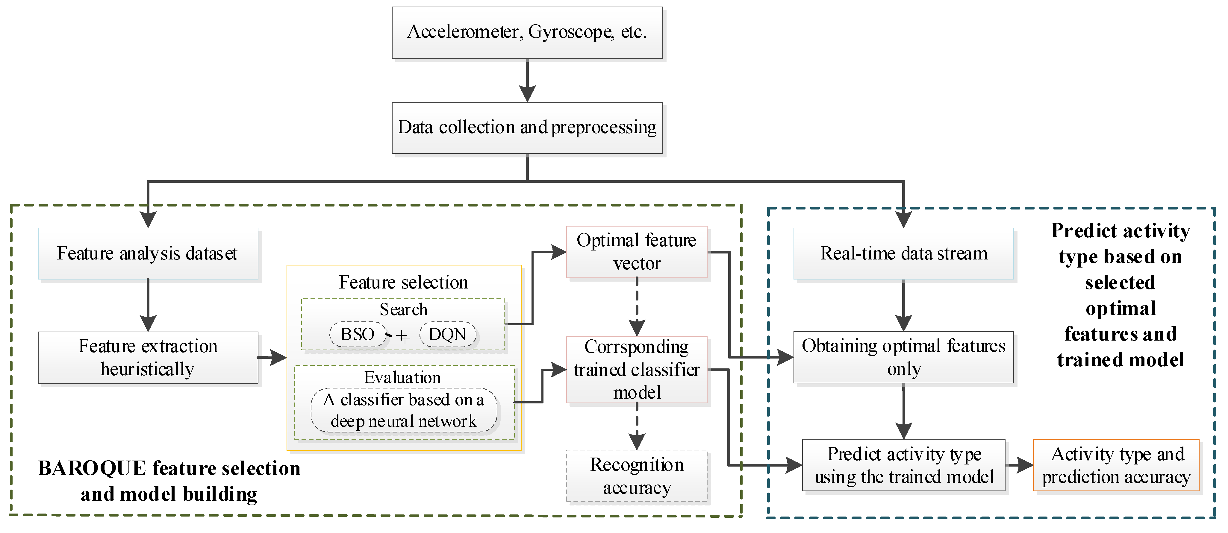
3. Proposed Method
3.1. Data Collection and Preprocessing
3.2. Feature Extraction
3.3. Feature Selection
3.3.1. Bee Swarm Optimization Metaheuristic
3.3.2. BSO for Feature Selection
3.3.3. Deep Q-Network
3.3.4. Multi-Agent DQN for Feature Selection
3.3.5. BAROQUE: The Proposed Hybrid Scheme
| Algorithm 1. Overall algorithm flow for BSO and BAROQUE. |
| Input: An instance of a combinatorial optimization problem Output: The best solution found 1: Initialize a reference solution, ref_sol, at random or via a heuristic 2: while not stopping criterion do 3: Determine search_region from ref_sol 4: Set the value of n_chances as max_chances 5: Assign a solution from search_region to each bee 6: for each bee b do 7: Carry out a local search 8: Store the result in the dance table 9: end for 10: if best_sol is better than best_global_sol then 11: Set the value of best_global_sol as best_sol 12: Set the value of n_chances as max_chances 13: Intensification 14: else 15: if n_chances > 0 then 16: n_chances minus one 17: Intensification 18: else 19: Diversification 20: end if 21: end if 22: end while 23: return best_global_sol |
3.4. Evaluation and Prediction
4. Experimental Results and Analysis
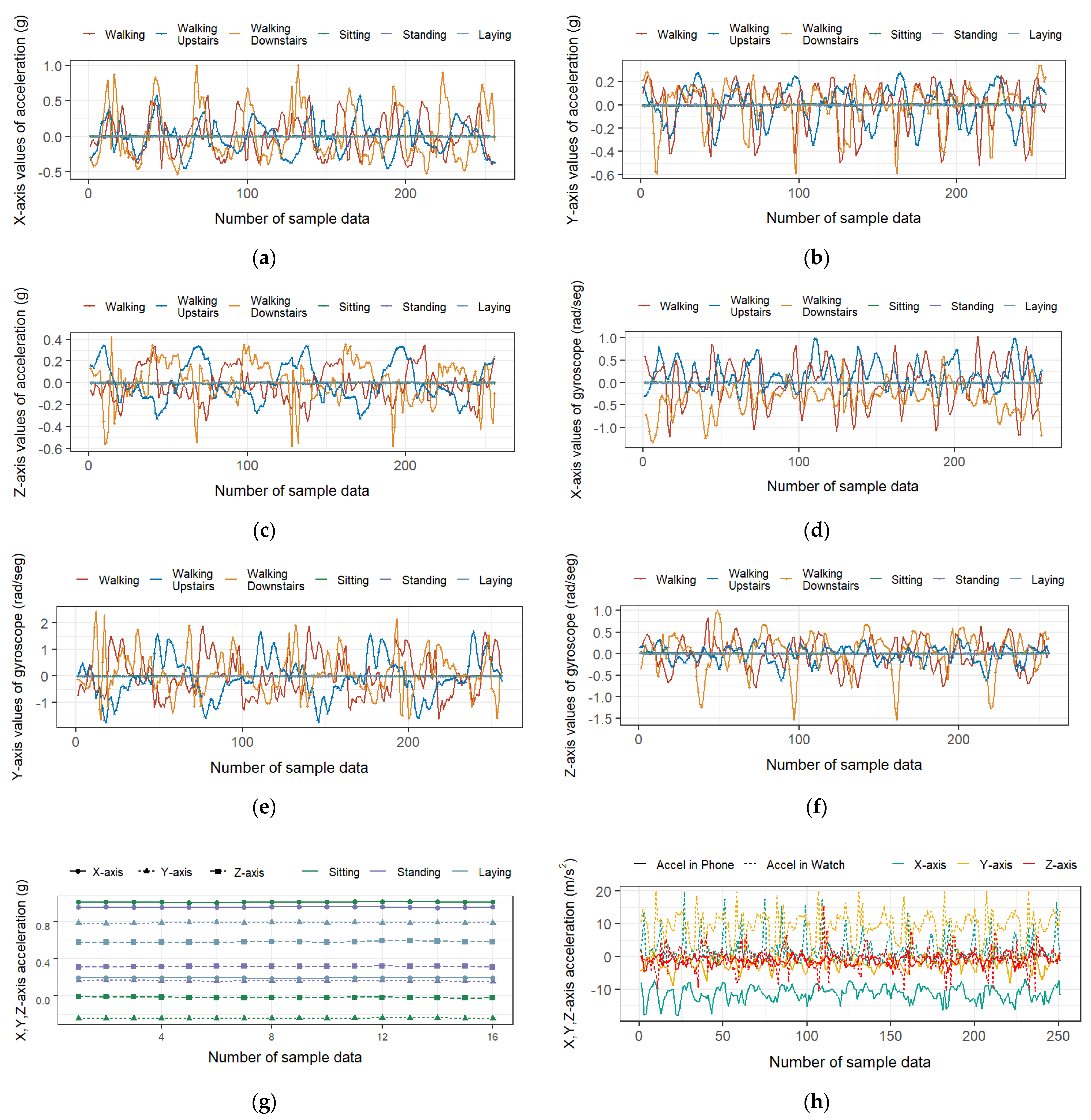
4.1. Analysis of Raw Signals
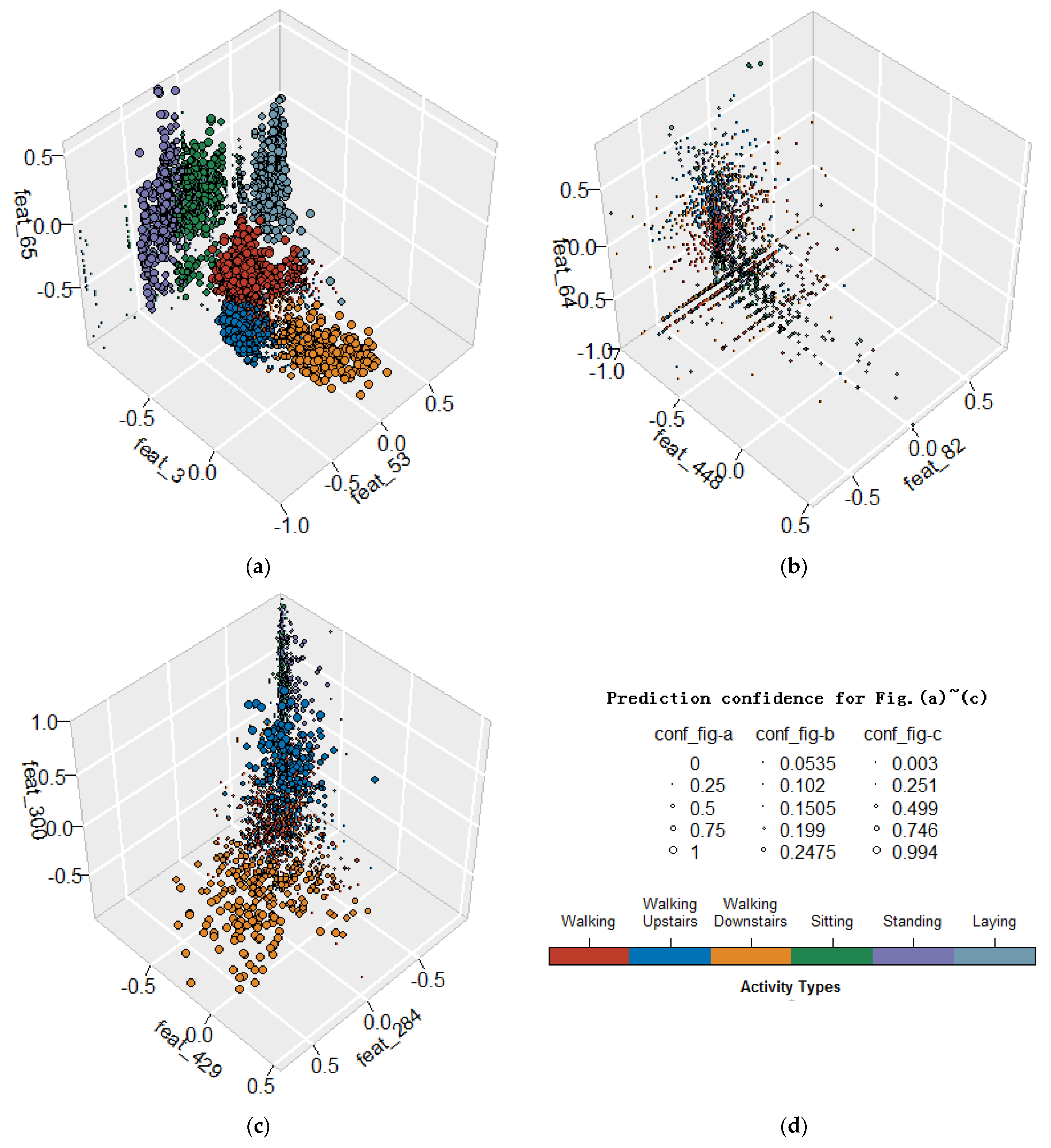
4.2. Analysis for Feature Selection
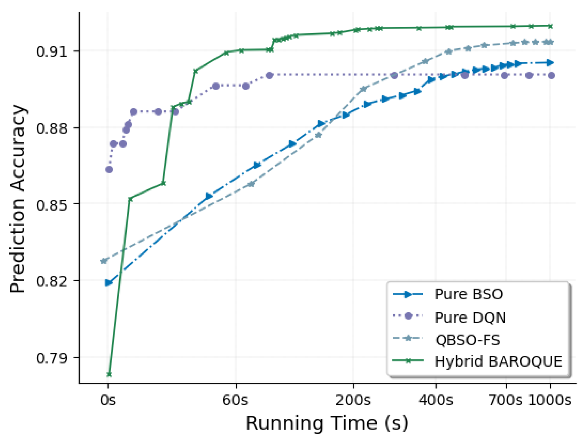
4.3. Analysis on Hybrid Combination
4.4. Comparison with Other Feature Selection Methods
4.5. Comparison with Other Swarm-Based Methods
4.6. Comparison with Other HAR Solutions
5. Conclusions
Author Contributions
Funding
Institutional Review Board Statement
Informed Consent Statement
Data Availability Statement
Conflicts of Interest
References
- Kim, E.; Helal, S.; Cook, D. Human activity recognition and pattern discovery. IEEE Pervasive Comput. 2009, 9, 48–53. [Google Scholar] [CrossRef] [Green Version]
- Osmani, V.; Balasubramaniam, S.; Botvich, D. Human activity recognition in pervasive health-care: Supporting efficient remote collaboration. J. Netw. Comput. Appl. 2008, 31, 628–655. [Google Scholar] [CrossRef]
- Tentori, M.; Favela, J. Activity-aware computing for healthcare. IEEE Pervasive Comput. 2008, 7, 51–57. [Google Scholar] [CrossRef]
- Al Machot, F.; Mosa, A.H.; Ali, M.; Kyamakya, K. Activity recognition in sensor data streams for active and assisted living environments. IEEE Trans. Circuits Syst. Video Technol. 2017, 28, 2933–2945. [Google Scholar] [CrossRef]
- Tosato, D.; Spera, M.; Cristani, M.; Murino, V. Characterizing humans on Riemannian manifolds. IEEE Trans. Pattern Anal. Mach. Intell. 2013, 35, 1972–1984. [Google Scholar] [CrossRef]
- Ramamurthy, S.R.; Roy, N. Recent trends in machine learning for human activity recognition—A survey. Interdiscipl. Rev. Data Mining Knowl. Discov. 2018, 8, e1245. [Google Scholar] [CrossRef]
- Foerster, F.; Smeja, M. Joint amplitude and frequency analysis of tremor activity. Electromyogr. Clin. Neuro-Physiol. 1999, 39, 11–19. [Google Scholar]
- Yu, H.; Cang, S.; Wang, Y. A review of sensor selection, sensor devices and sensor deployment for wearable sensor-based human activity recognition systems. In Proceedings of the 2016 10th International Conference on Software, Knowledge, Information Management & Applications (SKIMA), Chengdu, China, 15–17 December 2016. [Google Scholar]
- Shoaib, M.; Bosch, S.; Incel, O.D.; Scholten, J.; Havinga, P.J.M. Complex Human Activity Recognition Using Smartphone and Wrist-Worn Motion Sensors. Sensors 2016, 16, 426. [Google Scholar] [CrossRef] [PubMed]
- Mitra, U.; Emken, B.A.; Lee, S.; Li, M.; Rozgic, V.; Thatte, G.; Vathsangam, H.; Zois, D.-S.; Annavaram, M.; Narayanan, S.; et al. KNOWME: A case study in wireless body area sensor network design. IEEE Commun. Mag. 2012, 50, 116–125. [Google Scholar] [CrossRef]
- Wang, Y.; Cang, S.; Yu, H. A survey on wearable sensor modality centered human activity recognition in health care. Expert Syst. Appl. 2019, 137, 167–190. [Google Scholar] [CrossRef]
- Jordao, A.; Nazare, A.C.; Sena, J.; Schwartz, W.R. Human activity recognition based on wearable sensor data: A standardization of the state-of-the-art. arXiv 2018, arXiv:1806.05226. [Google Scholar]
- Slim, S.O.; Atia, A.; Elfattah, M.M.A.; M.Mostafa, M.-S. Survey on Human Activity Recognition based on Acceleration Data. Int. J. Adv. Comput. Sci. Appl. 2019, 10, 84–98. [Google Scholar] [CrossRef]
- Lara, O.D.; Labrador, M.A. A survey on human activity recognition using wearable sensors. IEEE Commun. Surv. Tutor. 2012, 15, 1192–1209. [Google Scholar] [CrossRef]
- Bao, L.; Intille, S.S. Activity recognition from user-annotated acceleration data. In Proceedings of the Pervasive Computing: Second International Conference (PERVASIVE 2004), Linz/Vienna, Austria, 21–23 April 2004; Springer: Berlin/Heidelberg, Germany, 2004; pp. 1–17. [Google Scholar]
- Tapia, E.M.; Intille, S.S.; Haskell, W.; Larson, K.; Wright, J.; King, A.; Friedman, R. Real-time recognition of physical activities and their intensities using wireless accelerometers and a heart monitor. In Proceedings of the International Symposium on Wearable Computers, Boston, MA, USA, 11–13 October 2007. [Google Scholar]
- Ermes, M.; Parkka, J.; Cluitmans, L. Advancing from offline to online activity recognition with wearable sensors. In Proceedings of the 30th Annual International Conference of the IEEE Engineering in Medicine and Biology Society, Vancouver, BC, Canada, 20–25 August 2008; pp. 4451–4454. [Google Scholar]
- Parkka, J.; Ermes, M.; Korpipaa, P.; Mäntyjärvi, J.; Peltola, J.; Korhonen, I. Activity Classification Using Realistic Data from Wearable Sensors. IEEE Trans. Inf. Technol. Biomed. 2006, 10, 119–128. [Google Scholar] [CrossRef]
- Berchtold, M.; Budde, M.; Gordon, D.; Schmidtke, H.; Beigl, M. Actiserv: Activity recognition service for mobile phones. In Proceedings of the International Symposium on Wearable Computers, Seoul, Korea, 10–13 October 2010; pp. 1–8. [Google Scholar]
- Reddy, S.; Mun, M.; Burke, J.; Estrin, D.; Hansen, M.; Srivastava, M. Using mobile phones to determine transportation modes. ACM Trans. Sens. Netw. 2010, 6, 1–27. [Google Scholar] [CrossRef]
- Chen, Y.; Shen, C. Performance Analysis of Smartphone-Sensor Behavior for Human Activity Recognition. IEEE Access 2017, 5, 3095–3110. [Google Scholar] [CrossRef]
- Hassan, M.M.; Uddin, M.Z.; Mohamed, A.; Almogren, A. A robust human activity recognition system using smartphone sensors and deep learning. Future Gener. Comput. Syst. 2018, 81, 307–313. [Google Scholar] [CrossRef]
- Ronao, C.A.; Cho, S.-B. Human activity recognition with smartphone sensors using deep learning neural networks. Expert Syst. Appl. 2016, 59, 235–244. [Google Scholar] [CrossRef]
- Wang, A.; Chen, G.; Yang, J.; Zhao, S.; Chang, C.-Y. A Comparative Study on Human Activity Recognition Using Inertial Sensors in a Smartphone. IEEE Sens. J. 2016, 16, 4566–4578. [Google Scholar] [CrossRef]
- Kwon, Y.; Kang, K.; Bae, C. Unsupervised learning for human activity recognition using smartphone sensors. Expert Syst. Appl. 2014, 41, 6067–6074. [Google Scholar] [CrossRef]
- Ronao, C.A.; Cho, S.-B. Human activity recognition using smartphone sensors with two-stage continuous hidden Markov models. In Proceedings of the 2014 10th International Conference on Natural Computation (ICNC), Xiamen, China, 19–21 August 2014; pp. 681–686. [Google Scholar]
- Chen, Z.; Zhu, Q.; Soh, Y.C.; Zhang, L. Robust Human Activity Recognition Using Smartphone Sensors via CT-PCA and Online SVM. IEEE Trans. Ind. Inform. 2017, 13, 3070–3080. [Google Scholar] [CrossRef]
- Paul, P.; George, T. An effective approach for human activity recognition on smartphone. In Proceedings of the 2015 IEEE International Conference on Engineering and Technology (ICETECH), Coimbatore, India, 20 March 2015; pp. 1–3. [Google Scholar]
- Cao, L.; Wang, Y.; Zhang, B.; Jin, Q.; Vasilakos, A.V. GCHAR: An efficient Group-based Context—Aware human activity recognition on smartphone. J. Parallel Distrib. Comput. 2018, 118, 67–80. [Google Scholar] [CrossRef]
- Mekruksavanich, S.; Hnoohom, N.; Jitpattanakul, A. Smartwatch-based sitting detection with human activity recognition for office workers syndrome. In Proceedings of the 2018 International ECTI Northern Section Conference on Electrical, Electronics, Computer and Telecommunications Engineering (ECTI-NCON), Chiang Rai, Thailand, 25–28 February 2018; pp. 160–164. [Google Scholar]
- Kwon, M.-C.; Choi, S. Recognition of daily human activity using an artificial neural network and smartwatch. Wirel. Commun. Mob. Comput. 2018, 2018, 2618045. [Google Scholar] [CrossRef]
- Ali, H.M.; Muslim, A.M. Human activity recognition using smartphone and smartwatch. Int. J. Comput. Eng. Res. Trends 2016, 3, 568–576. [Google Scholar] [CrossRef]
- Baldominos, A.; Cervantes, A.; Saez, Y.; Isasi, P. A Comparison of Machine Learning and Deep Learning Techniques for Activity Recognition using Mobile Devices. Sensors 2019, 19, 521. [Google Scholar] [CrossRef] [Green Version]
- Al-Janabi, S.; Salman, A.H. Sensitive integration of multilevel optimization model in human activity recognition for smartphone and smartwatch applications. Big Data Min. Anal. 2021, 4, 124–138. [Google Scholar] [CrossRef]
- Fan, C.; Gao, F. A new approach for smoking event detection using a variational autoencoder and neural decision forest. IEEE Access 2020, 8, 120835–120849. [Google Scholar] [CrossRef]
- Bulling, A.; Blanke, U.; Schiele, B. A tutorial on human activity recognition using body-worn inertial sensors. ACM Comput. Surv. 2014, 46, 1–33. [Google Scholar] [CrossRef]
- Jović, A.; Brkić, K.; Bogunović, N. A review of feature selection methods with applications. In Proceedings of the 38th International Convention on Information and Communication Technology, Electronics and Microelectronics (MIPRO), Opatija, Croatia, 25–29 May 2015. [Google Scholar]
- Suto, J.; Oniga, S.; Sitar, P.P. Comparison of wrapper and filter feature selection algorithms on human activity recognition. In Proceedings of the 2016 6th International Conference on Computers Communications and Control (ICCCC), Oradea, Romania, 10–14 May 2016; pp. 124–129. [Google Scholar]
- Zhang, M.; Sawchuk, A.A. A feature selection-based framework for human activity recognition using wearable multimodal sensors. In Proceedings of the 6th International Conference on Body Area Networks: Institute for Computer Sciences, Social-Informatics and Telecommunications Engineering, Beijing, China, 7–8 November 2011; pp. 92–98. [Google Scholar]
- Wang, A.; Chen, G.; Wu, X.; Liu, L.; An, N.; Chang, C.-Y. Towards Human Activity Recognition: A Hierarchical Feature Selection Framework. Sensors 2018, 18, 3629. [Google Scholar] [CrossRef] [Green Version]
- Zheng, Y. Human Activity Recognition Based on the Hierarchical Feature Selection and Classification Framework. J. Electr. Comput. Eng. 2015, 2015, 1–9. [Google Scholar] [CrossRef] [Green Version]
- Fang, H.; He, L.; Si, H.; Liu, P.; Xie, X. Human activity recognition based on feature selection in smart home using back-propagation algorithm. ISA Trans. 2014, 53, 1629–1638. [Google Scholar] [CrossRef]
- Capela, N.A.; Lemaire, E.; Baddour, N. Feature Selection for Wearable Smartphone-Based Human Activity Recognition with Able bodied, Elderly, and Stroke Patients. PLoS ONE 2015, 10, e0124414. [Google Scholar] [CrossRef] [Green Version]
- Fish, B.; Khan, A.; Chehade, N.H.; Chien, C.; Pottie, G. Feature selection based on mutual information for human activity recognition. In Proceedings of the 2012 IEEE International Conference on Acoustics, Speech and Signal Processing (ICASSP), Kyoto, Japan, 25–30 March 2012; pp. 1729–1732. [Google Scholar]
- Karagiannaki, K.; Panousopoulou, A.; Tsakalides, P. An online feature selection architecture for human activity recognition. In Proceedings of the 2017 IEEE International Conference on Acoustics, Speech and Signal Processing (ICASSP), New Orleans, LA, USA, 5–9 March 2017; pp. 2522–2526. [Google Scholar]
- Chowdhury, A.K.; Tjondronegoro, D.; Chandran, V.; Trost, S.G. Physical activity recognition using posterior-adapted class-based fusion of multiaccelerometer data. IEEE J. Biomed. Health Inform. 2017, 22, 678–685. [Google Scholar] [CrossRef]
- Zainudin, M.N.S.; Sulaiman, N.; Mustapha, N.; Perumal, T. Activity Recognition Using One-Versus-All Strategy with Relief-F and Self-Adaptive Algorithm. In Proceedings of the 2018 IEEE Conference on Open Systems (ICOS), Langkawi, Malaysia, 21–22 November 2018; pp. 31–36. [Google Scholar]
- Gupta, P.; Tim, D. Feature selection and activity recognition system using a single triaxial accelerometer. Biomed. Eng. IEEE Trans. 2014, 61, 1780–1786. [Google Scholar] [CrossRef]
- Altun, K.; Barshan, B. Human activity recognition using inertial/magnetic sensor units. In Proceedings of the 1st International Workshop on Human Behavior Understanding, Istanbul, Turkey, 22 August 2010; Springer: Berlin/Heidelberg, Germany, 2010; pp. 38–51. [Google Scholar]
- Leightley, D.; Darby, J.; Li, B.; McPhee, J.S.; Yap, M.H. Human Activity Recognition for Physical Rehabilitation. In Proceedings of the 2013 IEEE International Conference on Systems, Man, and Cybernetics, Manchester, UK, 13–16 October 2013; pp. 261–266. [Google Scholar]
- Kose, M.; Incel, O.D.; Ersoy, C. Online human activity recognition on smart phones. In Proceedings of the 2nd International Workshop on Mobile Sensing: From Smartphones and Wearables to Big Data, Beijing, China, 16 April 2012; pp. 11–15. [Google Scholar]
- Yang, J.; Nguyen, M.N.; San, P.P.; Li, X.L.; Krishnaswamy, S. Deep convolutional neural networks on multichannel time series for human activity recognition. In Proceedings of the Twenty-Fourth International Joint Conference on Artificial Intelligence, Buenos Aires, Argentina, 25–31 July 2015. [Google Scholar]
- Hammerla, N.Y.; Halloran, S.; Plötz, T. Deep, convolutional, and recurrent models for human activity recognition using wearables. arXiv 2016, arXiv:1604.08880. [Google Scholar]
- Chen, K.; Zhang, D.; Yao, L.; Guo, B.; Yu, Z.; Liu, Y. Deep Learning for Sensor-based Human Activity Recognition: Overview, Challenges, and Opportunities. ACM Comput. Surv. CSUR 2021, 54, 1–40. [Google Scholar]
- Chen, K.; Yao, L.; Zhang, D.; Guo, B.; Yu, Z. Multi-agent Attentional Activity Recognition. In Proceedings of the Twenty-Eighth International Joint Conference on Artificial Intelligence, Macao, China, 10–16 August 2019. [Google Scholar]
- Chen, K.; Yao, L.; Wang, X.; Zhang, D.; Gu, T.; Yu, Z.; Yang, Z. Interpretable Parallel Recurrent Neural Networks with Convolutional Attentions for Multi-Modality Activity Modeling. In Proceedings of the 2018 International Joint Conference on Neural Networks (IJCNN), Rio de Janeiro, Brazil, 8–13 July 2018; pp. 1–8. [Google Scholar]
- Bhat, G.; Deb, R.; Chaurasia, V.V.; Shill, H.; Ogras, U.Y. Online human activity recognition using low-power wearable devices. In Proceedings of the Proceedings of the International Conference on Computer-Aided Design, San Diego, CA, USA, 5–8 November 2018; pp. 1–8. [Google Scholar]
- Kabir, M.; Shahjahan, M.; Murase, K. A new hybrid ant colony optimization algorithm for feature selection. Expert Syst. Appl. 2012, 39, 3747–3763. [Google Scholar] [CrossRef]
- Rostami, M.; Moradi, P. A clustering based genetic algorithm for feature selection. In Proceedings of the 2014 6th Conference on Information and Knowledge Technology (IKT), Shahrood, Iran, 27–29 May 2014; pp. 112–116. [Google Scholar]
- Xue, B.; Zhang, M.; Browne, W.N. Browne. Particle swarm optimisation for feature selection in classification: Novel initialisation and updating mechanisms. Appl. Soft Comput. 2014, 18, 261–276. [Google Scholar] [CrossRef]
- Sadeg, S.; Hamdad, L.; Benatchba, K.; Habbas, Z. BSO-FS: Bee swarm optimization for feature selection in classification. In Advances in Computational Intelligence, Proceedings of the International Work-Conference on Artificial Neural Networks, Palma de Mallorca, Spain, 10–12 June 2015; Springer: Berlin/Heidelberg, Germany; pp. 387–399.
- Sadeg, S.; Hamdad, L.; Remache, A.R.; Karech, M.N.; Benatchba, K.; Habbas, A. Qbso-fs: A reinforcement learning based bee swarm optimization metaheuristic for feature selection. In Advances in Computational Intelligence, Proceedings of the International Work-Conference on Artificial Neural Networks; Springer: Berlin/Heidelberg, Germany, 2019; pp. 785–796. [Google Scholar]
- Anguita, D.; Ghio, A.; Oneto, L.; Parra, X.; Reyes-Ortiz, J.L. A public domain dataset for human activity recognition using smartphones. In Proceedings of the 21th European Symposium on Artificial Neural Networks, Computational Intelligence and Machine Learning, ESANN 2013, Bruges, Belgium, 24–26 April 2013. [Google Scholar]
- Weiss, G.M.; Kenichi, Y.; Thaier, H. Smartphone and smartwatch-based biometrics using activities of daily living. IEEE Access 2019, 7, 133190–133202. [Google Scholar] [CrossRef]
- Fong, S.; Liang, J.; Fister, I.; Mohammed, S. Gesture recognition from data streams of human motion sensor using accelerated PSO swarm search feature selection algorithm. J. Sens. 2015, 2015, 205707. [Google Scholar] [CrossRef]
- Saputri, T.R.; Khan, A.M.; Lee, S. User-Independent Activity Recognition via Three-Stage GA-Based Feature Selection. Int. J. Distrib. Sens. Netw. 2014, 10, 706287. [Google Scholar] [CrossRef]
- Li, J.; Tian, L.; Chen, L.; Wang, H.; Cao, T.; Yu, L. Optimal Feature Selection for Activity Recognition based on Ant Colony Algorithm. In Proceedings of the Conference on Industrial Electronics and Applications, Xi’an, China, 19–21 June 2019. [Google Scholar]
- Myo, W.W.; Wettayaprasit, W.; Aiyarak, P. A Cyclic Attribution Technique Feature Selection Method for Human Activity Recognition. Int. J. Intell. Syst. Appl. 2019, 10, 25–32. [Google Scholar] [CrossRef]
- Ahmed, N.; Rafiq, J.I.; Islam, M.R. Enhanced human activity recognition based on smartphone sensor data using hybrid feature selection model. Sensors 2020, 20, 317. [Google Scholar] [CrossRef] [Green Version]


| Extracted Features | Equation | Extracted Features | Equation |
|---|---|---|---|
| Mean | Cross Correlation | ||
| Variance | Frequency Center | FC = | |
| Absolute Mean Value | Energy | E = | |
| SRA | = | Entropy | H |
| Standard Deviation | RMS Frequency | ||
| Zero Crossing Rate | ZC = | Minimum | Min |
| Median | Maximum | Max | |
| Interquartile Range | IQR = | Peak to Peak | PPV = Max |
| Root Mean Square | Impulse Factor | IF = | |
| Correlation coefficient | = | Margin Factor | MF = |
| Skewness | SV = | Shape Factor | SF = |
| Kurtosis | KV = | Crest Factor | CF = |
| Walking | Walking Upstairs | Walking Downstairs | Sitting | Standing | Laying | |
|---|---|---|---|---|---|---|
| T3 | 18.55% | 25.69% | 24.05% | 19.14% | 20.3% | 23.28% |
| R3 | 52.82% | 46.71% | 32.62% | 54.79% | 67.86% | 42.27% |
| W3 | 88.51% | 100% | 100% | 99.79% | 49.06% | 74.86% |
| Smartphone Sensor Data | Smartwatch Sensor Data | |
|---|---|---|
| Used Activities | clapping, writing, eating soup, climbing stairs, folding clothes, playing catch, dribbling a basketball and kicking a soccer ball | |
| Selected Features | Feature number of sfp: 0,2,3,5,6,7,9,12,14,15,20,21,22,23,25,33, 35,36,37,39,40,42,43,44,45,46,47,49,50,53, 55,56,59,60,61,63,65,66,68,69,70,71,73, 78,80,81,88,89,90,91,92,104,105,109,118, 119,122,125,127,128,129,133,135,136,138, 139,141,145,148,150,152,155,156,159, 161,164,169,171,175,178,179,180,181 | Feature number of sfw: 0,5,9,10,11,15,16,20,21,27,31,36,45,50,51, 54,58,59,61,64,70,76,80,81,82,85,86,90, 91,96,98,99,105,108,110,111,116,123,125, 126,128,130,131,137,141,145,146,148,150, 151,156,158,160,161,164,166,167,168, 172,178,181 |
| Accuracy using sfp | 92.22% | 93.49% |
| Accuracy using sfw | 86.01% | 95.35% |
| Joint Features | 0,5,9,15,20,21,36,45,50,59,61,70,80,81,90,91,105,125,128,141,145,148,150,156,161,164,178,181 | |
| Overlap Ratio | 0.337 (28/83) | 0.459 (28/61) |
| Algorithms | Need All Features | Time Cost (s) | Prediction Accuracy (%) |
|---|---|---|---|
| PCA | Yes | 1.38 | 99.65% |
| kPCA | Yes | 100.2 | 99.65% |
| Relief-F | No | 161.74 | 99.83% |
| CFS | No | 6147.22 | 95.54% |
| SFFS | No | 160,817.5 | 99.98% |
| BAROQUE | No | 32.46 | 99.91% |
| Dataset | No-FS | GA | BPSO | ACO | BAROQUE |
|---|---|---|---|---|---|
| UCI-HAR | 97.86% | 97.37% | 97.48% | 97.38% | 97.48% |
| WISDM_W | 81.09% | 78.60% | 80.00% | 76.12% | 80.93% |
| WISDM_A | 89.30% | 86.35% | 88.84% | 87.91% | 88.99% |
| UT_complex | 99.83% | 99.83% | 99.91% | 99.83% | 99.91% |
| BAROQUE | SMC-SVM | MC-SVM | Convnet | CAT | |
|---|---|---|---|---|---|
| walking | 98.84% | 98.99% | 99% | 98.99% | 89.24% |
| walking downstairs | 98.34% | 98.33% | 98% | 100% | 100% |
| walking upstairs | 99.37% | 97.24% | 96% | 100% | 94.52% |
| standing | 95.98% | 97.18% | 97% | 93.23% | 99.19% |
| sitting | 97.94% | 97.76% | 88% | 88.80% | 99.08% |
| laying | 100% | 99.26% | 100% | 87.71% | 99.12% |
| Average | 98.41% | 98.13% | 96% | 94.79% | 96.86% |
Publisher’s Note: MDPI stays neutral with regard to jurisdictional claims in published maps and institutional affiliations. |
© 2021 by the authors. Licensee MDPI, Basel, Switzerland. This article is an open access article distributed under the terms and conditions of the Creative Commons Attribution (CC BY) license (https://creativecommons.org/licenses/by/4.0/).
Share and Cite
Fan, C.; Gao, F. Enhanced Human Activity Recognition Using Wearable Sensors via a Hybrid Feature Selection Method. Sensors 2021, 21, 6434. https://doi.org/10.3390/s21196434
Fan C, Gao F. Enhanced Human Activity Recognition Using Wearable Sensors via a Hybrid Feature Selection Method. Sensors. 2021; 21(19):6434. https://doi.org/10.3390/s21196434
Chicago/Turabian StyleFan, Changjun, and Fei Gao. 2021. "Enhanced Human Activity Recognition Using Wearable Sensors via a Hybrid Feature Selection Method" Sensors 21, no. 19: 6434. https://doi.org/10.3390/s21196434
APA StyleFan, C., & Gao, F. (2021). Enhanced Human Activity Recognition Using Wearable Sensors via a Hybrid Feature Selection Method. Sensors, 21(19), 6434. https://doi.org/10.3390/s21196434