
Estimating Fuel Moisture in Grasslands Using UAV-Mounted Infrared and Visible Light Sensors

 , , and
Abstract
:
1. Introduction
2. Materials and Methods
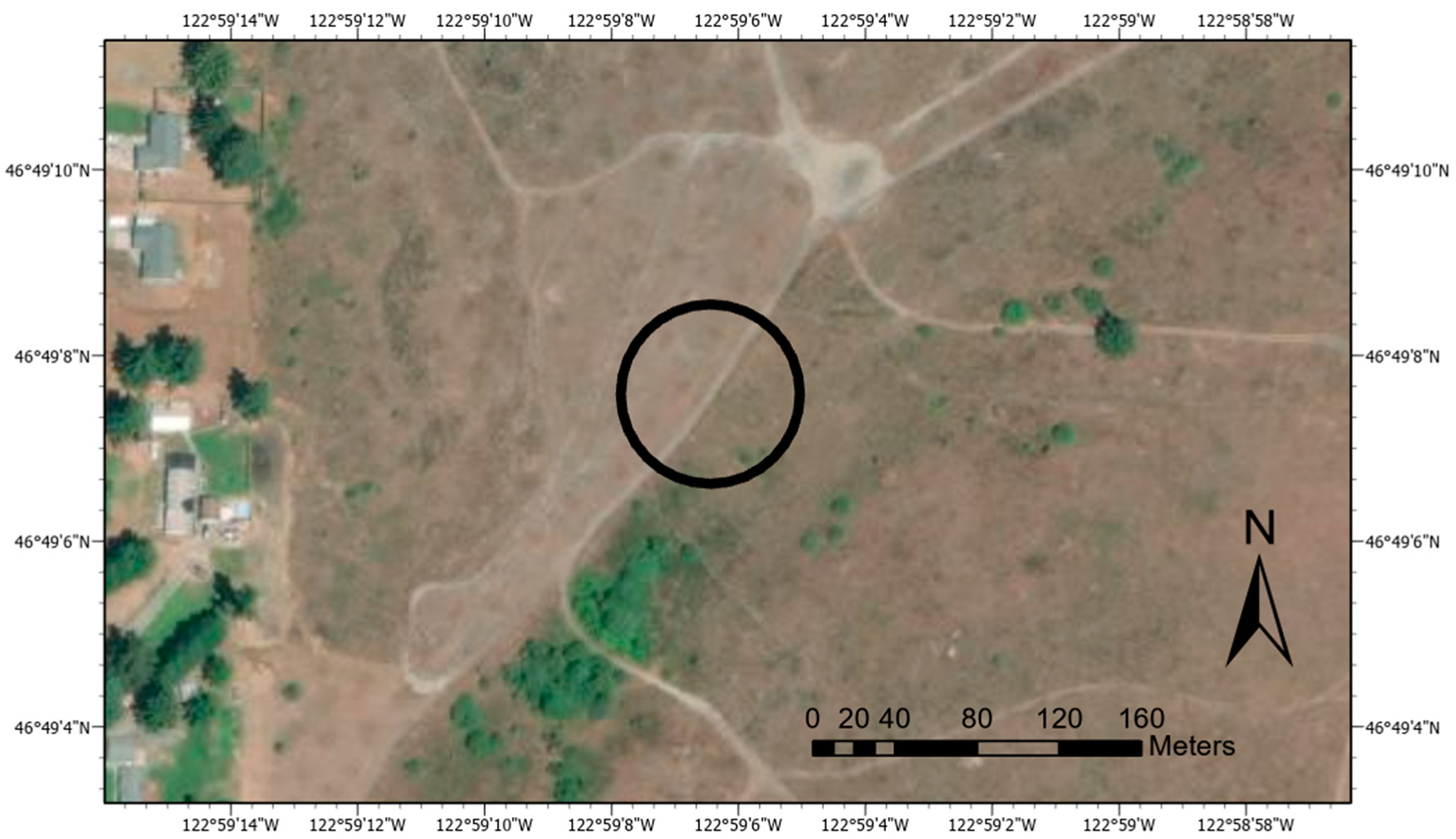
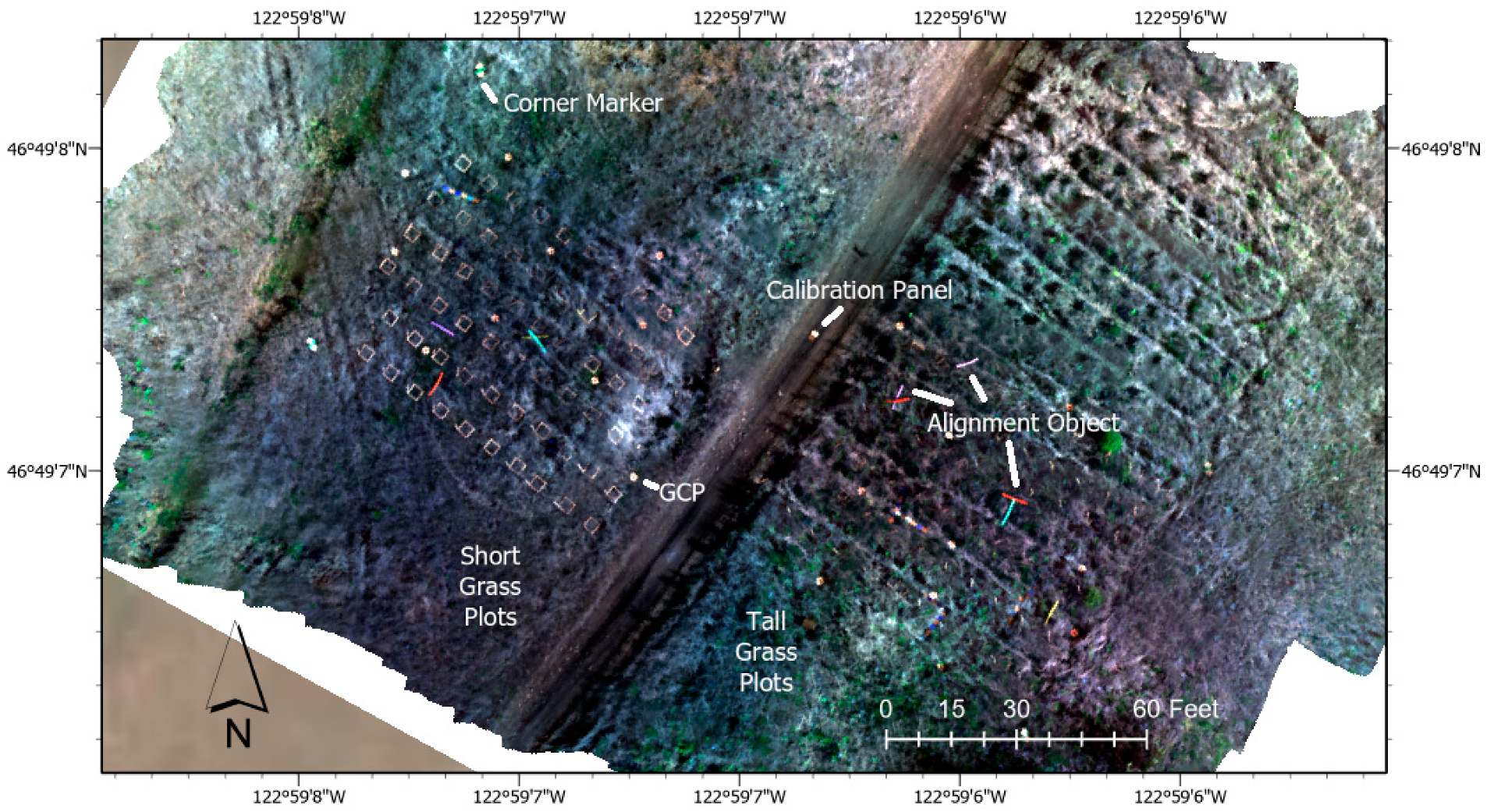
2.1. Site Selection
2.2. Imagery Data Collection
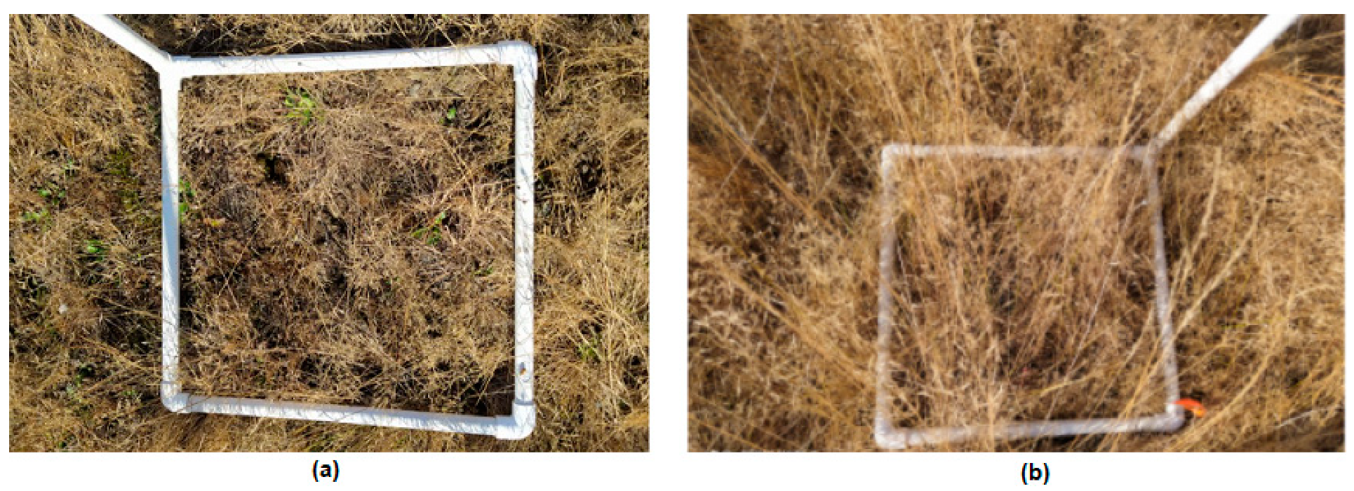
2.3. Field Data Collection
2.4. Pre-Processing Methods
2.5. Statistical Analysis
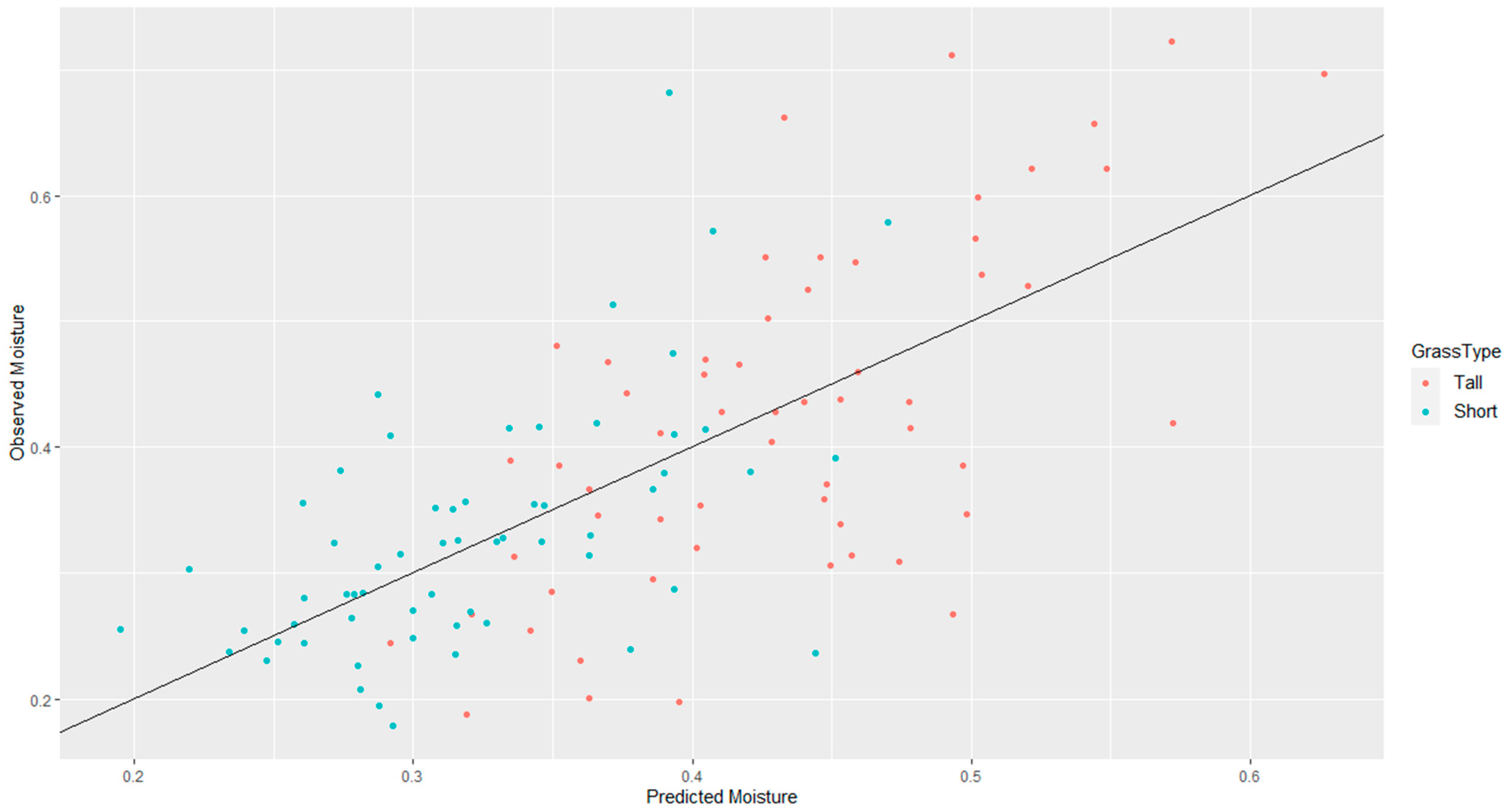
3. Results
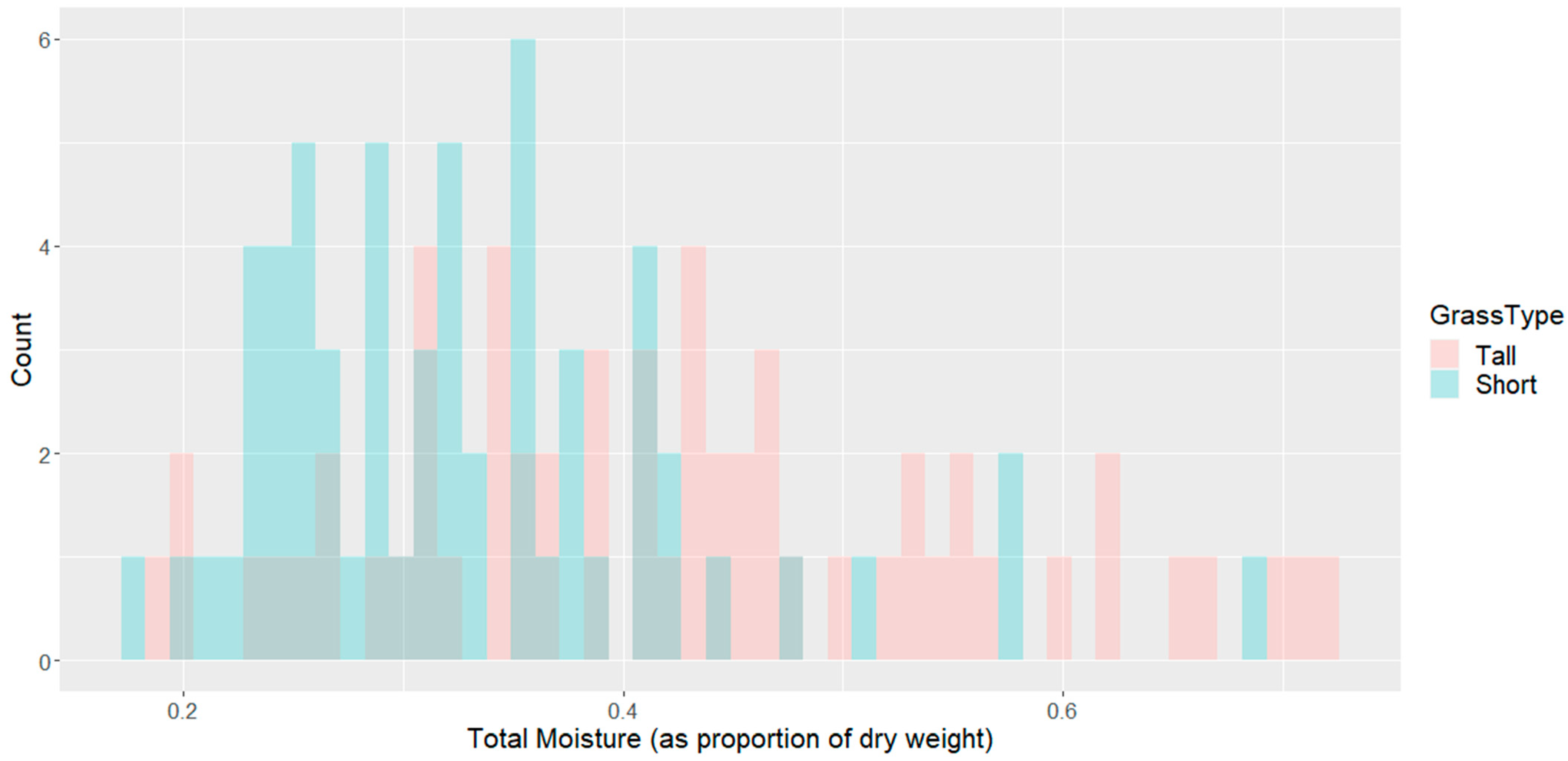
3.1. Comparison of Moisture Measurement Methods
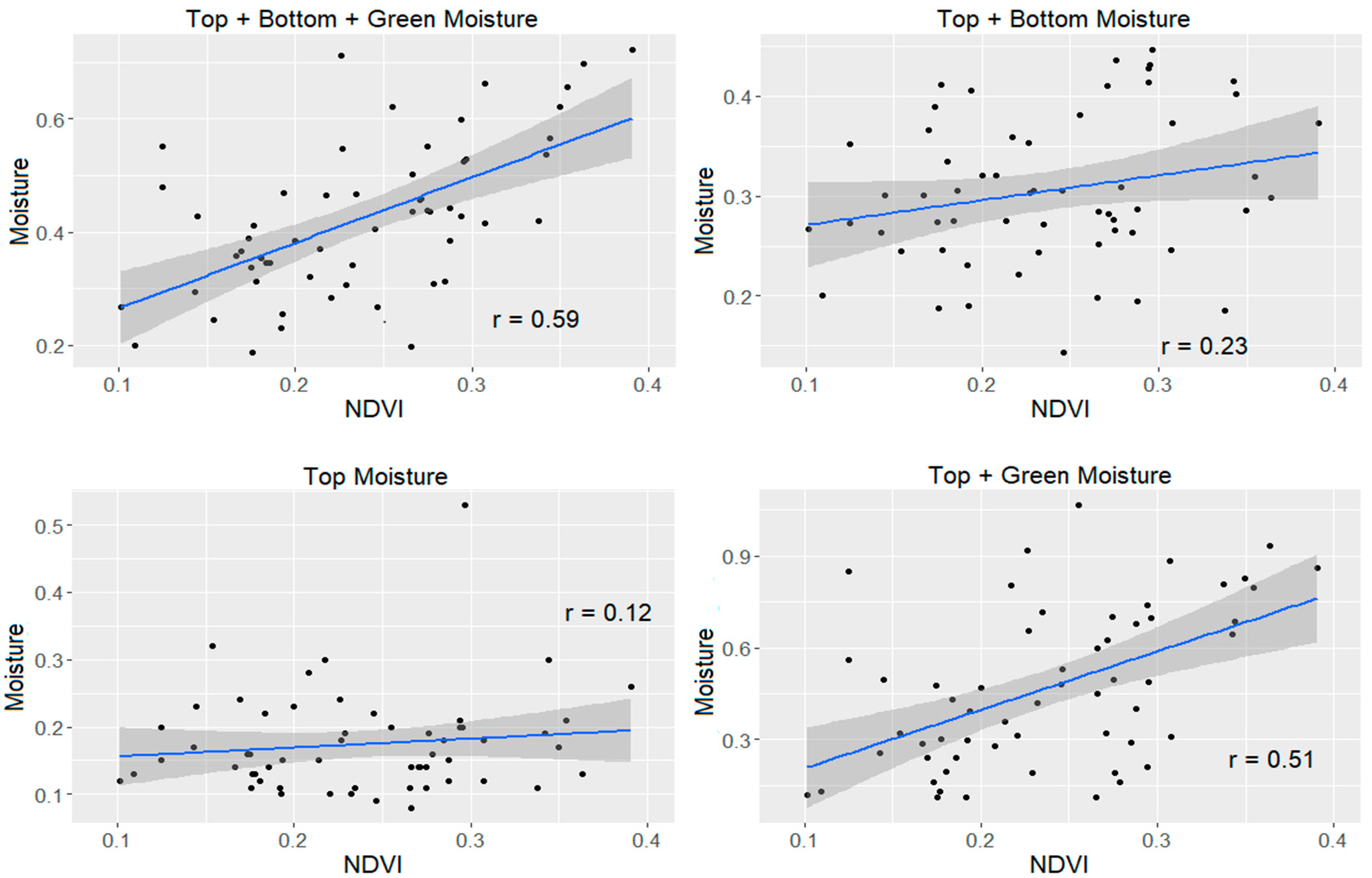
3.2. Model Building
4. Discussion
4.1. Comparison of Models
4.2. Implications for Sensor Selection
4.3. Future Improvements of Method
4.4. Future Work
5. Conclusions
Supplementary Materials
Author Contributions
Funding
Institutional Review Board Statement
Informed Consent Statement
Data Availability Statement
Acknowledgments
Conflicts of Interest
References
- Yebra, M.; Dennison, P.E.; Chuvieco, E.; Riaño, D.; Zylstra, P.; Raymond Hunt, E.; Mark Danson, F.; Qi, Y.; Jurdao, S. A global review of remote sensing of live fuel moisture content for fire danger assessment: Moving towards operational products. Remote Sens. Environ. 2013, 136, 455–468. [Google Scholar] [CrossRef]
- Mell, W.; McNamara, D.; Maranghides, A.; McDermott, R.; Forney, G.; Hoffman, C.; Ginder, M. Computer modelling of wildland-urban interface fires. In Proceedings of the Fire and Materials, San Francisco, CA, USA, 31 January–2 February 2011. [Google Scholar]
- Larkin, N.K.; O’Neill, S.M.; Solomon, R.; Raffuse, S.; Strand, T.; Sullivan, D.C.; Krull, C.; Rorig, M.; Peterson, J.; Ferguson, S.A. The BlueSky smoke modeling framework. Int. J. Wildland Fire 2009, 18, 906. [Google Scholar] [CrossRef] [Green Version]
- Coen, J.L.; Natasha Stavros, E.; Fites-Kaufman, J.A. Deconstructing the King megafire. Ecol. Appl. 2018, 28, 1565–1580. [Google Scholar] [CrossRef] [PubMed]
- Gillett, N.P. Detecting the effect of climate change on Canadian forest fires. Geophys. Res. Lett. 2004, 31. [Google Scholar] [CrossRef] [Green Version]
- Heyerdahl, E.K.; Alvarado, E. Influence of Climate and Land Use on Historical Surface Fires in Pine-Oak Forests, Sierra Madre Occidental, Mexico. In Fire and Climatic Change in Temperate Ecosystems of the Western Americas; Springer: New York, NY, USA, 2003; Volume 160, pp. 196–217. [Google Scholar]
- Hammer, R.B.; Radeloff, V.C.; Fried, J.S.; Stewart, S.I. Wildland—Urban interface housing growth during the 1990s in California, Oregon, and Washington. Int. J. Wildland Fire 2007, 16, 255. [Google Scholar] [CrossRef] [Green Version]
- Mell, W.E.; Manzello, S.L.; Maranghides, A.; Butry, D.; Rehm, R.G. The wildland—Urban interface fire problem—Current approaches and research needs. Int. J. Wildland Fire 2010, 19, 238. [Google Scholar] [CrossRef]
- Biswell, H. Prescribed Burning in California Wildlands Vegetation Management; University of California Press: Berkeley, CA, USA, 1999; ISBN 9780520219458. [Google Scholar]
- Fernandes, P.M. Empirical Support for the Use of Prescribed Burning as a Fuel Treatment. Curr. For. Rep. 2015, 1, 118–127. [Google Scholar] [CrossRef] [Green Version]
- Crecente-Campo, F.; Pommerening, A.; Rodríguez-Soalleiro, R. Impacts of thinning on structure, growth and risk of crown fire in a Pinus sylvestris L. plantation in northern Spain. For. Ecol. Manag. 2009, 257, 1945–1954. [Google Scholar] [CrossRef]
- Brown, T.J.; Hall, B.L.; Westerling, A.L. The Impact of Twenty-First Century Climate Change on Wildland Fire Danger in the Western United States: An Applications Perspective. Clim. Chang. 2004, 62, 365–388. [Google Scholar] [CrossRef]
- Livingston, A.C.; Morgan Varner, J. Fuel Moisture Differences in a Mixed Native and Non-Native Grassland: Implications for Fire Regimes. Fire Ecol. 2016, 12, 73–87. [Google Scholar] [CrossRef]
- Jolly, W.M.; Matt Jolly, W. Sensitivity of a surface fire spread model and associated fire behaviour fuel models to changes in live fuel moisture. Int. J. Wildland Fire 2007, 16, 503. [Google Scholar] [CrossRef] [Green Version]
- Chuvieco, E.; Aguado, I.; Dimitrakopoulos, A.P. Conversion of fuel moisture content values to ignition potential for integrated fire danger assessment. Can. J. For. Res. 2004, 34, 2284–2293. [Google Scholar] [CrossRef]
- Anderson, S.A.J.; Anderson, W.R. Ignition and fire spread thresholds in gorse (Ulex europaeus). Int. J. Wildland Fire 2010, 19, 589. [Google Scholar] [CrossRef]
- Maki, M.; Ishiahra, M.; Tamura, M. Estimation of leaf water status to monitor the risk of forest fires by using remotely sensed data. Remote Sens. Environ. 2004, 90, 441–450. [Google Scholar] [CrossRef]
- Schowengerdt, R.A. Remote Sensing: Models and Methods for Image Processing; Elsevier: Amsterdam, The Netherlands, 2012; ISBN 9780080516103. [Google Scholar]
- Torresan, C.; Berton, A.; Carotenuto, F.; Di Gennaro, S.F.; Gioli, B.; Matese, A.; Miglietta, F.; Vagnoli, C.; Zaldei, A.; Wallace, L. Forestry applications of UAVs in Europe: A review. Int. J. Remote. Sens. 2017, 38, 2427–2447. [Google Scholar] [CrossRef]
- Banu, T.P.; Borlea, G.F.; Banu, C. The Use of Drones in Forestry. J. Environ. Sci. Eng. B 2016, 5, 557–562. [Google Scholar]
- Rothermel, R.C. A Mathematical Model for Predicting Fire Spread in Wildland Fuels; Intermountain Forest and Range Experiment Station: Ogden, UT, USA, 1972. [Google Scholar]
- Balbi, J.H.; Morandini, F.; Silvani, X.; Filippi, J.B.; Rinieri, F. A physical model for wildland fires. Combust. Flame 2009, 156, 2217–2230. [Google Scholar] [CrossRef] [Green Version]
- McGrattan, K.B.; McDermott, R.; Weinschenk, C.; Overholt, K.; Hostikka, S.; Floyd, J. Fire Dynamics Simulator Technical Reference Guide; National Institute of Standards and Technology: Gaithersburg, MD, USA, 2013; Volume 1.
- Mell, W.; Jenkins, M.A.; Gould, J.; Cheney, P. A physics-based approach to modelling grassland fires. Int. J. Wildland Fire 2007, 16, 1. [Google Scholar] [CrossRef]
- Hudak, A.T.; Kato, A.; Bright, B.C.; Louise Loudermilk, E.; Hawley, C.; Restaino, J.C.; Ottmar, R.D.; Prata, G.A.; Cabo, C.; Prichard, S.J.; et al. Towards Spatially Explicit Quantification of Pre- and Postfire Fuels and Fuel Consumption from Traditional and Point Cloud Measurements. For. Sci. 2020, 66, 428–442. [Google Scholar] [CrossRef]
- Haase, S.M.; Sánchez, J.; Weise, D.R. Evaluation of Standard Methods for Collecting and Processing Fuel Moisture Samples; USDA Forest Service: Albany, CA, USA, 2016.
- Wang, L.; Raymond Hunt, E.; Qu, J.J.; Hao, X.; Daughtry, C.S.T. Remote sensing of fuel moisture content from ratios of narrow-band vegetation water and dry-matter indices. Remote Sens. Environ. 2013, 129, 103–110. [Google Scholar] [CrossRef] [Green Version]
- Elachi, C.; Zimmerman, P.D. Introduction to the physics and techniques of remote sensing. Phys. Today 1988, 41, 126. [Google Scholar] [CrossRef]
- Marino, E.; Yebra, M.; Guillén-Climent, M.; Algeet, N.; Tomé, J.L.; Madrigal, J.; Guijarro, M.; Hernando, C. Investigating Live Fuel Moisture Content Estimation in Fire-Prone Shrubland from Remote Sensing Using Empirical Modelling and RTM Simulations. Remote Sens. 2020, 12, 2251. [Google Scholar] [CrossRef]
- Stow, D.; Niphadkar, M.; Kaiser, J. Time series of chaparral live fuel moisture maps derived from MODIS satellite data. Int. J. Wildland Fire 2006, 15, 347. [Google Scholar] [CrossRef]
- Hao, X.; Qu, J. Retrieval of real-time live fuel moisture content using MODIS measurements. Remote Sens. Environ. 2007, 108, 130–137. [Google Scholar] [CrossRef]
- Chuvieco, E.; Riaño, D.; Aguado, I.; Cocero, D. Estimation of fuel moisture content from multitemporal analysis of Landsat Thematic Mapper reflectance data: Applications in fire danger assessment. Int. J. Remote Sens. 2002, 23, 2145–2162. [Google Scholar] [CrossRef]
- Danson, F.M.; Bowyer, P. Estimating live fuel moisture content from remotely sensed reflectance. Remote Sens. Environ. 2004, 92, 309–321. [Google Scholar] [CrossRef]
- Yebra, M.; Chuvieco, E.; Riaño, D. Estimation of live fuel moisture content from MODIS images for fire risk assessment. Agric. For. Meteorol. 2008, 148, 523–536. [Google Scholar] [CrossRef]
- Dennison, P.E.; Roberts, D.A.; Peterson, S.H.; Rechel, J. Use of Normalized Difference Water Index for monitoring live fuel moisture. Int. J. Remote Sens. 2005, 26, 1035–1042. [Google Scholar] [CrossRef]
- Peterson, S.; Roberts, D.; Dennison, P. Mapping live fuel moisture with MODIS data: A multiple regression approach. Remote Sens. Environ. 2008, 112, 4272–4284. [Google Scholar] [CrossRef]
- Stow, D.; Niphadkar, M. Stability, normalization and accuracy of MODIS-derived estimates of live fuel moisture for southern California chaparral. Int. J. Remote Sens. 2007, 28, 5175–5182. [Google Scholar] [CrossRef]
- Caccamo, G.; Chisholm, L.A.; Bradstock, R.A.; Puotinen, M.L.; Pippen, B.G. Monitoring live fuel moisture content of heathland, shrubland and sclerophyll forest in south-eastern Australia using MODIS data. Int. J. Wildland Fire 2012, 21, 257. [Google Scholar] [CrossRef]
- Rowlands, A. Physics of Digital Photography; IOP Publishing: Bristol, UK, 2017; ISBN 9780750312431. [Google Scholar]
- Sandino, J.; Gonzalez, F.; Mengersen, K.; Gaston, K.J. UAVs and Machine Learning Revolutionising Invasive Grass and Vegetation Surveys in Remote Arid Lands. Sensors 2018, 18, 605. [Google Scholar] [CrossRef] [PubMed] [Green Version]
- Viljanen, N.; Honkavaara, E.; Näsi, R.; Hakala, T.; Niemeläinen, O.; Kaivosoja, J. A Novel Machine Learning Method for Estimating Biomass of Grass Swards Using a Photogrammetric Canopy Height Model, Images and Vegetation Indices Captured by a Drone. Agriculture 2018, 8, 70. [Google Scholar] [CrossRef] [Green Version]
- Xiang, H.; Tian, L. Development of a low-cost agricultural remote sensing system based on an autonomous unmanned aerial vehicle (UAV). Biosyst. Eng. 2011, 108, 174–190. [Google Scholar] [CrossRef]
- Klemas, V.; Smart, R. The influence of soil salinity, growth form, and leaf moisture on the spectral radiance of Spartina Alterniflora Canopies. Photogramm. Eng. Remote Sens. 1983, 49, 77–83. [Google Scholar]
- Hardy, C.C.; Burgan, R.E. Evaluation of NDVI for monitoring live moisture in three vegetation types of the western US. Photogramm. Eng. Remote Sens. 1999, 65, 603–610. [Google Scholar]
- Jenal, A.; Bareth, G.; Bolten, A.; Kneer, C.; Weber, I.; Bongartz, J. Development of a VNIR/SWIR multispectral imaging system for vegetation monitoring with unmanned aerial vehicles. Sensors 2019, 19, 5507. [Google Scholar] [CrossRef] [PubMed] [Green Version]
- Gruszczyński, W.; Puniach, E.; Ćwiąkała, P.; Matwij, W. Application of convolutional neural networks for low vegetation filtering from data acquired by UAVs. ISPRS J. Photogramm. Remote Sens. 2019, 158, 1–10. [Google Scholar] [CrossRef]
- Manly, B.F.J.; Navarro Alberto, J.A. Multivariate Statistical Methods: A Primer, Fourth Edition; CRC Press: Boca Raton, FL, USA, 2016; ISBN 9781498728997. [Google Scholar]
- Lim, J.; Watanabe, N.; Yoshitoshi, R.; Kawamura, K. Simple in-field evaluation of moisture content in curing forage using normalized differece vegetation index (NDVI). Grassl. Sci. 2020, 66, 238–248. [Google Scholar] [CrossRef]
- Qi, J.; Chehbouni, A.; Huete, A.R.; Kerr, Y.H.; Sorooshian, S. A modified soil adjusted vegetation index. Remote Sens. Environ. 1994, 48, 119–126. [Google Scholar] [CrossRef]
- Gao, B.-C. NDWI—A normalized difference water index for remote sensing of vegetation liquid water from space. Remote Sens. Environ. 1996, 58, 257–266. [Google Scholar] [CrossRef]
- Zhang, H.; Ma, S.; Kang, P.; Zhang, Q.; Wu, Z. Spatial heterogeneity of dead fuel moisture content in a Larix gmelinii forest in Inner Mongolia using geostatistics. J. For. Res. 2021, 32, 569–577. [Google Scholar] [CrossRef]
- Kennard, D.K.; Outcalt, K. Modeling spatial patterns of fuels and fire behavior in a longleaf pine forest in the Southeastern USA. Fire Ecol. 2006, 2, 31–52. [Google Scholar] [CrossRef]
- White, J.C.; Coops, N.C.; Wulder, M.A.; Vastaranta, M.; Hilker, T.; Tompalski, P. Remote sensing technologies for enhancing forest inventories: A review. Can. J. Remote Sens. J. Can. Teledetect. 2016, 42, 619–641. [Google Scholar] [CrossRef] [Green Version]
- Näsi, R.; Viljanen, N.; Kaivosoja, J.; Alhonoja, K.; Hakala, T.; Markelin, L.; Honkavaara, E. Estimating biomass and nitrogen amount of barley and grass using UAV and aircraft based spectral and photogrammetric 3D features. Remote Sens. 2018, 10, 1082. [Google Scholar] [CrossRef] [Green Version]
- Walter, J.; Edwards, J.; McDonald, G.; Kuchel, H. Photogrammetry for the estimation of wheat biomass and harvest index. Field Crops Res. 2018, 216, 165–174. [Google Scholar] [CrossRef]
- Devia, C.A.; Rojas, J.P.; Petro, E.; Martinez, C.; Mondragon, I.F.; Patino, D.; Rebolledo, M.C.; Colorado, J. High-throughput biomass estimation in rice crops using UAV multispectral imagery. J. Intell. Robot. Syst. 2019, 96, 573–589. [Google Scholar] [CrossRef]
- Harkel, J.T.; Bartholomeus, H.; Kooistra, L. Biomass and crop height estimation of different crops using UAV-based LiDAR. Remote Sens. 2019, 12, 17. [Google Scholar] [CrossRef] [Green Version]


| Name | Formula |
|---|---|
| NDVI | (NIR − Red)/(NIR + Red) |
| NDWI | (NIR − SWIR)/(NIR + SWIR) |
| VARI | (Green − Red)/(Green + Red − Blue) |
| NDGR | (Green − Red)/(Green + Red) |
| Band | Wavelength Range | Wavelength of MODIS Band |
|---|---|---|
| Red (MS) | 668 ± 7 nm | 645 ± 25 nm |
| Green (MS) | 560 ± 13.5 nm | 550 ± 10 nm |
| Blue (MS) | 475 ±16 nm | 488 ± 5 nm |
| NIR (MS) | 842 ± 28 nm | 858 ± 17 nm |
| Red Edge (MS) | 717 ± 6 nm | NA |
| SWIR (Tau) | 1300 ± 400 nm | 1240 ± 10 nm |
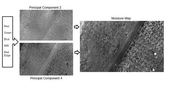
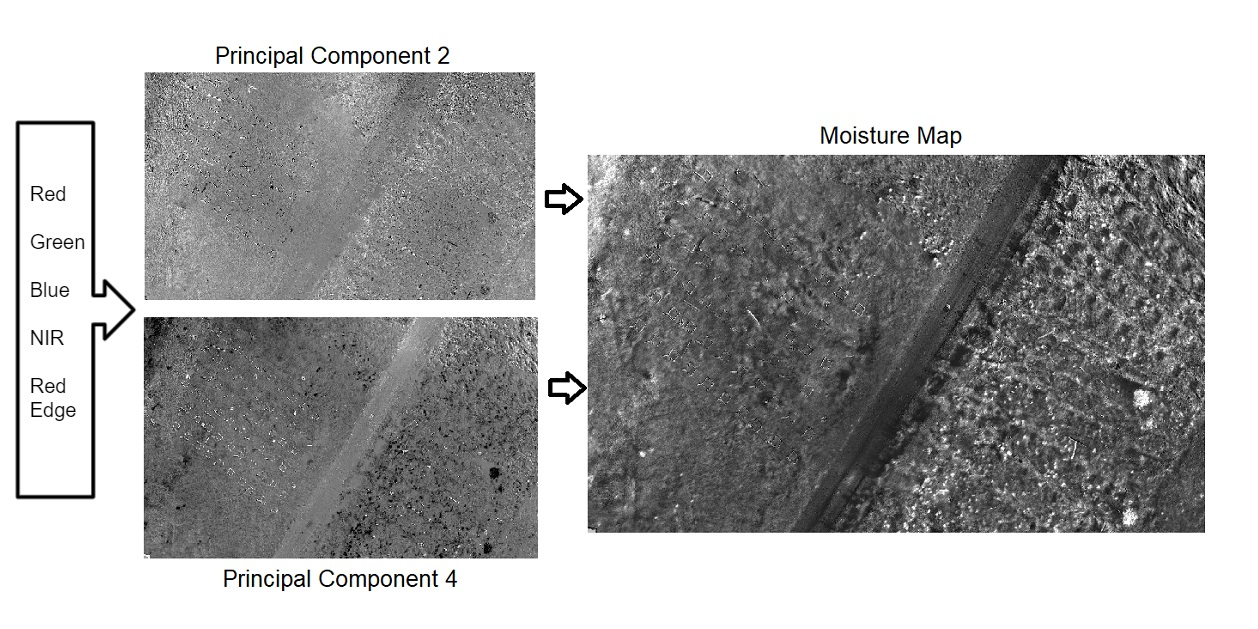
| PC1 | PC2 | PC3 | PC4 | |
|---|---|---|---|---|
| Red | 0.462 | 0.222 | 0.403 | 0.670 |
| Green | 0.460 | 0.622 | −0.625 | |
| Blue | 0.408 | 0.746 | −0.474 | −0.225 |
| Red Edge | 0.438 | −0.317 | −0.185 | 0.296 |
| NIR | 0.464 | −0.540 | −0.438 | −0.152 |
| % Variation | 0.848 | 0.090 | 0.034 | 0.018 |
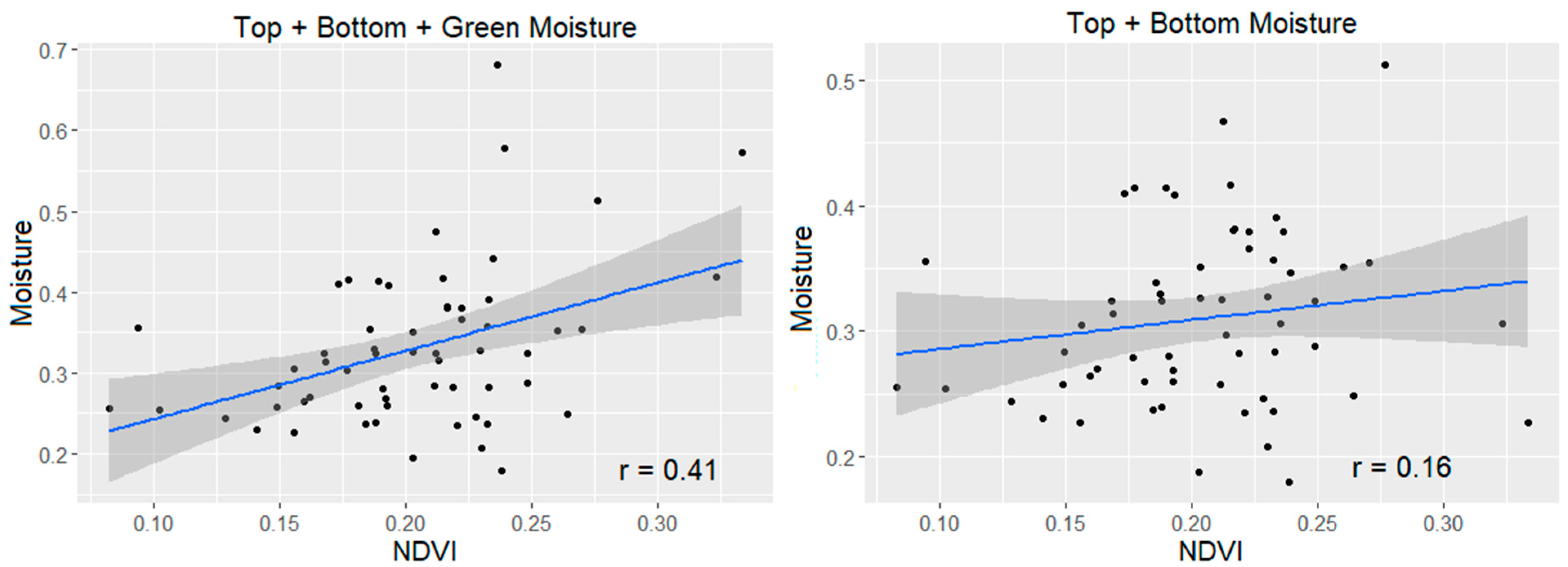
| Index | Adj. r² | Slope | Intercept | p-Value |
|---|---|---|---|---|
| NDVI | 0.329 | 1.189 | 0.115 | 0.000 |
| NDWI | 0.014 | −0.085 | 0.374 | 0.119 |
| VARI | 0.174 | 0.571 | 0.377 | 0.000 |
| NDGR | 0.174 | 0.956 | 0.376 | 0.000 |
| NDVI + Weight | 0.431 | 0.930 0.001 | 0.093 | 0.000 |
| NDWI + Weight | 0.307 | −0.027 0.002 | 0.253 | 0.000 |
| VARI + Weight | 0.303 | 0.340 0.001 | 0.285 | 0.000 |
| NDGR + Weight | 0.304 | 0.570 0.001 | 0.285 | 0.000 |
| PC2 | 0.336 | −0.124 | 0.380 | 0.000 |
| PC2 + PC4 | 0.387 | −0.133 −0.106 | 0.381 | 0.000 |
| PC2 + PC4 + Weight | 0.452 | −0.105 −0.091 0.001 | 0.315 | 0.000 |
| PC1 + PC2 + PC3 + PC4 +Weight | 0.467 | −0.004 −0.112 −0.046 −0.099 0.001 | 0.316 | 0.000 |
| Index | Dominant Species | Adj. r² | Slope | Intercept | p-Value |
|---|---|---|---|---|---|
| NDVI | A. elatius | 0.340 | 1.157 | 0.150 | 0.000 |
| A. stolonifera | 0.154 | 0.843 | 0.159 | 0.001 | |
| VARI | A. elatius | 0.037 | 0.403 | 0.406 | 0.078 |
| A.stolonifera | 0.128 | 0.438 | 0.351 | 0.002 | |
| NDVI + Weight | A. elatius | 0.372 | 1.045 0.001 | 0.081 | 0.000 |
| A. stolonifera | 0.258 | 0.717 0.001 | 0.121 | 0.000 | |
| PC2 + PC4 + Weight | A. elatius | 0.435 | −0.141 −0.080 0.001 | 0.288 | 0.000 |
| A. stolonifera | 0.316 | −0.084 −0.079 0.001 | 0.295 | 0.000 |
Publisher’s Note: MDPI stays neutral with regard to jurisdictional claims in published maps and institutional affiliations. |
© 2021 by the authors. Licensee MDPI, Basel, Switzerland. This article is an open access article distributed under the terms and conditions of the Creative Commons Attribution (CC BY) license (https://creativecommons.org/licenses/by/4.0/).
Share and Cite
Barber, N.; Alvarado, E.; Kane, V.R.; Mell, W.E.; Moskal, L.M. Estimating Fuel Moisture in Grasslands Using UAV-Mounted Infrared and Visible Light Sensors. Sensors 2021, 21, 6350. https://doi.org/10.3390/s21196350
Barber N, Alvarado E, Kane VR, Mell WE, Moskal LM. Estimating Fuel Moisture in Grasslands Using UAV-Mounted Infrared and Visible Light Sensors. Sensors. 2021; 21(19):6350. https://doi.org/10.3390/s21196350
Chicago/Turabian StyleBarber, Nastassia, Ernesto Alvarado, Van R. Kane, William E. Mell, and L. Monika Moskal. 2021. "Estimating Fuel Moisture in Grasslands Using UAV-Mounted Infrared and Visible Light Sensors" Sensors 21, no. 19: 6350. https://doi.org/10.3390/s21196350
APA StyleBarber, N., Alvarado, E., Kane, V. R., Mell, W. E., & Moskal, L. M. (2021). Estimating Fuel Moisture in Grasslands Using UAV-Mounted Infrared and Visible Light Sensors. Sensors, 21(19), 6350. https://doi.org/10.3390/s21196350