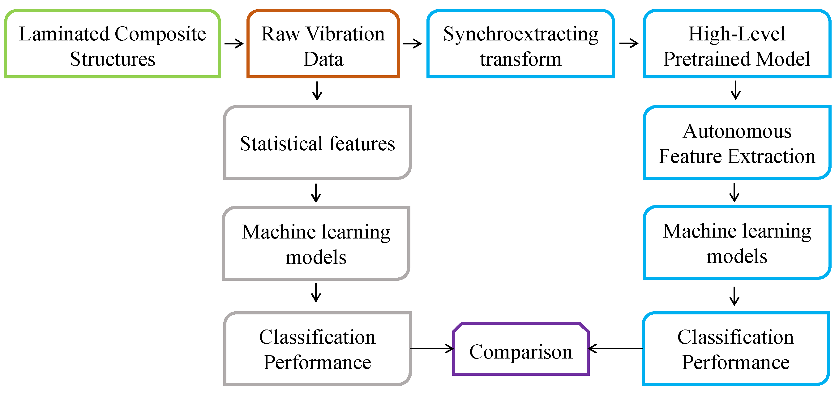
This section discusses the classification results into different health states for the laminated composite samples in the simulations and experiments based on both handcrafted statistical features and autonomously extracted features.
3.1. Classification Results on Handcrafted Statistical Features
Time and frequency domain statistical features of the signals have been used to discriminate between different health states of bearings, gearboxes, and rotating machines [
38,
39,
40,
41]. However, statistical features may not allow us to discriminate between the health states of laminated composites where the dynamic response is dominated by the excitation forces and the response signal may not reveal sufficient information to diagnose the characteristics of the fault present when analyzed in a conventional manner. To show the feasibility of using handcrafted statistical features to discriminate between different health states in the simulated data, time and frequency domain features were extracted from the time series data and analyzed through various machine learning algorithms. A window function of 0.2 s was employed to divide the random response signals over the 2 s period into 10 chunks. The purpose of this division is to look for discriminative features in a smaller portion of the signals instead of looking at the entire signal. The handcrafted time domain features used were the mean, standard deviation, skewness, kurtosis, peak to peak values, root mean squared values, crest factor, shape factor, impulse factor, margin factor, and energy of the signal. The extracted frequency domain features were the spectral kurtosis, spectral mean, spectral standard deviation, spectral skewness, and spectral kurtosis. The fifteen features were extracted from numerical data on the composite laminate samples in all five health states. The data from all samples in the various health states amounted to 1000 instances with 15 features for each instance. The values for the hand-crafted features in each instance was processed with different machine learning algorithms,
Table 3 depicts the performance of the different classifiers used to process those values in terms of training/validation accuracy and area under the receiver operating characteristics curve (ROC area).
All the classifiers were trained using a 10-fold cross-validation strategy. The results in
Table 3 show that the maximum classification accuracy using these statistical features was 43.8% achieved by Fine KNN. However, the ROC area, which reflects the tradeoff between the true positive and false positive rates of the classifiers, indicates that Fine KNN is susceptible to overfitting and will not generalize well to new, unseen data.
Although the classification accuracy is not high enough for practical applications, the training/validation confusion matrix may provide additional insights into the classification performance achieved.
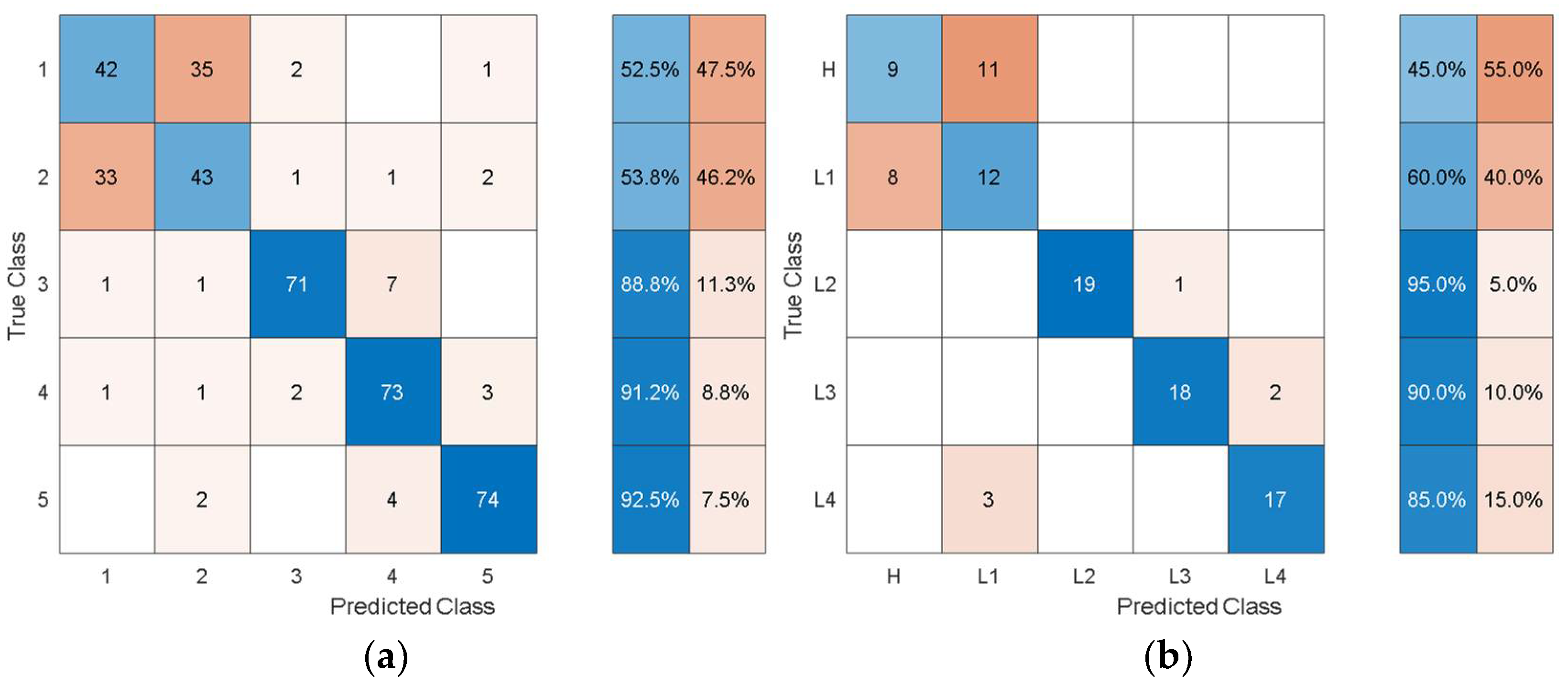
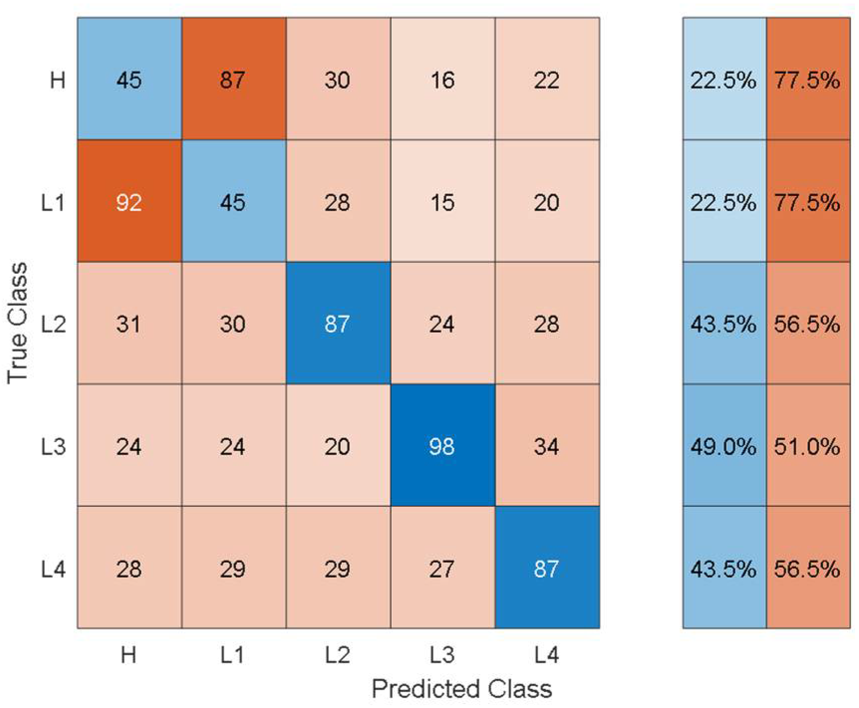
Figure 6 shows the training/validation confusion matrix of Cubic SVM.
In the confusion matrices, the values on the main diagonal denote correctly classified instances and the off-diagonal cells contain the misclassified instances. The blue and red columns on the right side show the recall (true-positive rate) and false-negative rate respectively, for each of the health states. Quantitatively, the recall gives the successful detection and isolation of a given health state while the false negative gives the susceptibility of a model to confusing other health states with the actual health state. From
Figure 6, it can be observed that though the classification accuracy is not very high, the classification results are consistent with the physics of the problem. For instance, the classifier can distinguish more severe cases of delamination (L2, L3, L4) with relatively higher classification accuracy and the major loss of accuracy comes from confusion between healthy and less severe cases of delamination i.e., confusion between H and L1.
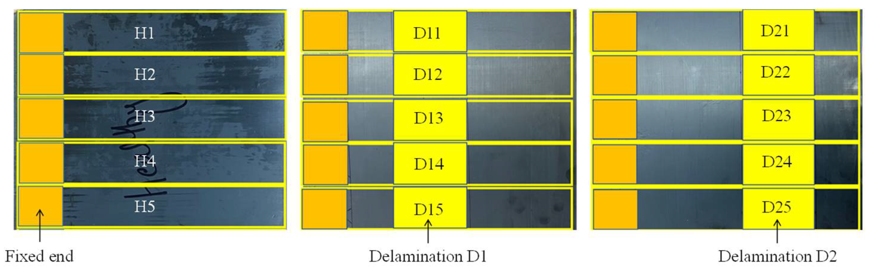
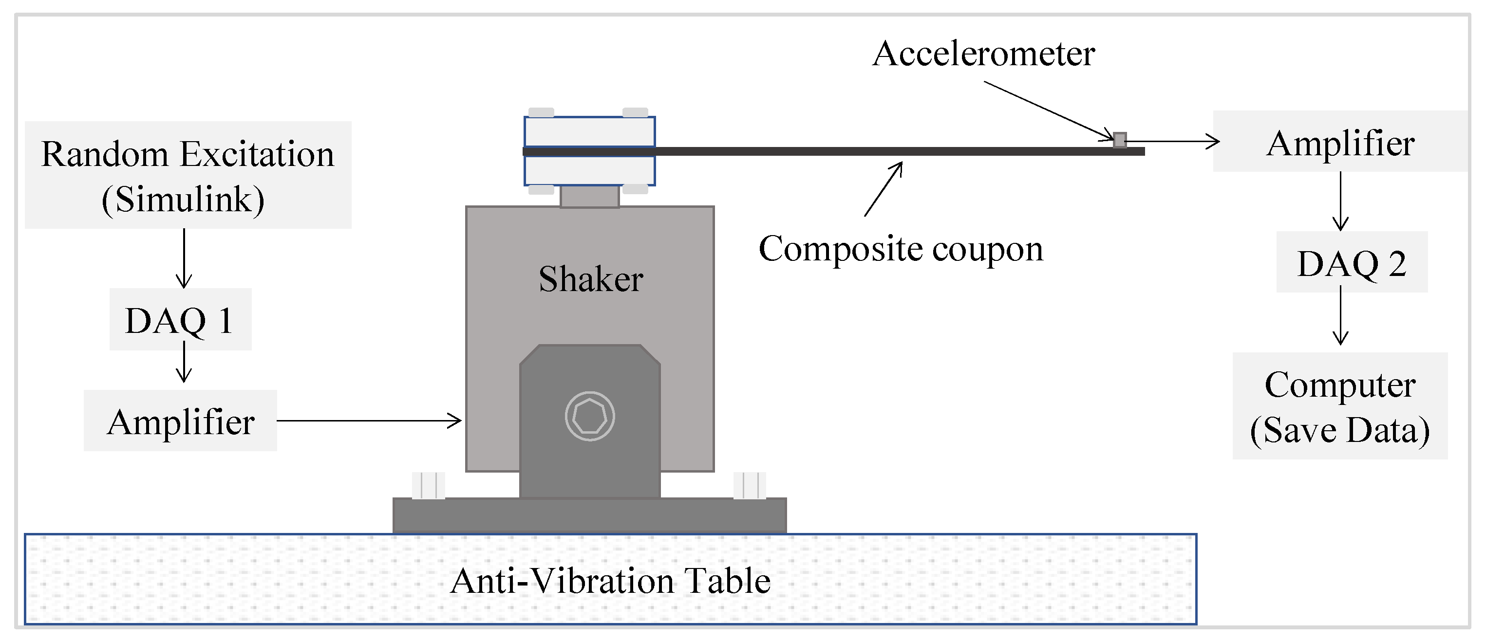
Experimental data was collected over a period of 15 s, the signal for each sample in each health state was split into 20 chunks using a window of 1875 data points. This created 100 instances for the five samples in each health state, resulting in a total of 300 instances for the three health states. The same statistical features used with the simulated data were extracted from the experimental data and were again processed using various machine learning algorithms.
Table 4 shows the performance results for each of the classifiers in terms of training/validation accuracy and area under the receiver operating characteristics curve (ROC area). All classifiers were trained using a 10-fold cross-validation strategy.
The result in the table shows that delaminations of the same size but at different locations can be correctly classified with a maximum classification accuracy of around 70 %. However, a classifier trained with this accuracy may be susceptible to high misclassification rates when deployed for making predictions on new data.
To give an idea of the per-class misclassification results,
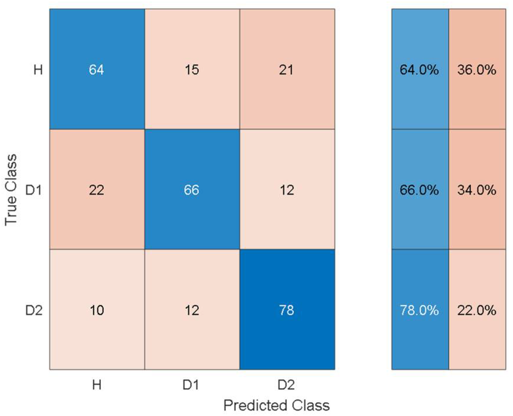
Figure 7 depicts the training/validation confusion matrix for the Fine Tree classifier.
It can be observed that the classifier can distinguish the three health states with 64%, 66%, and 78% classification accuracy. Furthermore, the susceptibility to misclassification was 36%, 34%, and 22% for the three health states.
Although the statistical features provide physically consistent results, the low classification accuracy when using these features hinders their practical application for the detection and isolation of delamination from low-frequency structural vibration in laminated composites. The next section shows the results of using discriminative features that were extracted autonomously via pretrained deep learning models.
3.2. Results from Using Features Extracted Autonomously Using Pretrained Deep Learning Models
In the deep learning framework, pretrained models can be employed for three purposes: to make predictions on new unseen data that is similar to previous data, for feature extraction using the activations of deep layers as features, and for transfer learning based on fine tuning a network that was pretrained on data from a different but related task to work with limited new data [
42,
43]. In this work, pretrained deep learning models based on AlexNet, GoogleNet, SqueezeNet, ResNet-18, and VGG-16 were employed for autonomous feature extraction from the limited data gathered by simulations and experiments. The reason for choosing different pretrained models for the current problem was to show the effect of the architecture, depth, and the number of pretrained deep learning model parameters for the fault diagnosis in a transfer learning framework. The characteristics features of the adopted pretrained models are shown in
Table 5.
Herein, it is observed that each network has different architectural characteristics, and one can choose a pretrained model based on the initial assessment of the results from different models, depth of the models, memory size, predictive performance, and prediction speed. A detailed description of the architecture of different pretrained deep learning models can be found in the references [
44,
45,
46].
The mathematical details of autonomous feature extraction via pretrained deep learning models are not discussed here for the sake of brevity but can be found in references [
47,
48,
49]. The autonomous features were processed via a quadratic support vector machine using 10-fold cross validation and a one-vs-all training strategy for the detection, quantification, and localization of delamination in laminated composites. The mathematical details of SVM for the assessment of discriminative features and classification results can be found in the references [
50,
51,
52].
Since the existing deep learning models were pretrained on image data, the time domain signals were transformed into time-frequency images using the Synchroextracting Transform (SET) technique introduced by Yu et al. [
26]. The reason for choosing SET instead of short-time Fast Fourier Transforms (STFT) or wavelet scalograms was that SET provided better time-frequency resolution. The mathematical details of encoding time series data into an image with SET can be found in references [
26,
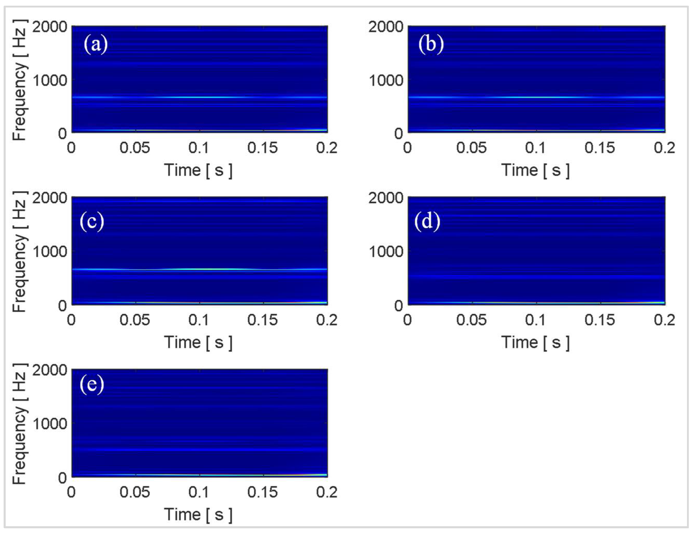
27]. The SET window length is the parameter that affects the time-frequency resolution. In the current work, after trying various lengths of SET windows, a window length equal to the length of the signal was found to provide the best time-frequency resolution for laminated composites. The time series data, windowed into smaller chunks in the same way as for the statistical features, was processed with SET to obtain time-frequency images representing the simulated and experimental data. Some representative time-frequency images of the simulated data obtain through SET are shown in
Figure 8.
The time-frequency images show different characteristic spectrums for each of the five health states. However, due to the random nature of the response signals, it is difficult to differentiate the health states from their time-frequency images using the naked eye. Moreover, the images in
Figure 8 are some representative examples from the 100 images for each health state and only correspond to a single random response signal. The difficulty level is further increased as the number of random excitations and their corresponding responses increase. Owing to their inherent architecture, deep learning models can look for minute differences between images allowing them to differentiate similar looking images autonomously with high accuracy. In the current work, the total number of images is only 500 (100 images for each health state), which is not sufficient to optimize the parameters of a deep learning model which is being developed and trained from scratch. Hence, in this work, off-the-shelf pretrained deep learning models were employed for autonomous feature extraction.
The autonomous features extracted at different layers of the pretrained models have different dimensions and discriminative capabilities. In the current work, features from different layers of the pretrained models are leveraged to discriminate between different health states of the laminated composites based on the simulated and experimental data. To ensure a consistent parametric study, the autonomous features were processed with quadratic SVM,
Table 6,
Table 7,
Table 8,
Table 9 and
Table 10 show its performance based on the autonomous features extracted from the simulated data in terms of training/validation accuracy, test accuracy, and the number of autonomous features.
It can be observed that the dimensions of the discriminative features are increasing as the feature extraction layer is moved from the final layers to the inner layers towards the initial layers of the pretrained models. In this problem, the accuracy is not affected much by whether high-level features (i.e., features from the last layers) or low-level features (i.e., features from the inner and initial layers) are used. However, the dimensions and consequently the computational cost of using the low-level features are higher than for using the high-level features. When compared with the classification performance using the hand-crafted statistical features shown in
Table 3, the performance using the autonomous features has substantially increased for all the pretrained models. To get further insights into the classification performance,
Figure 9,
Figure 10,
Figure 11,
Figure 12 and
Figure 13 depict the confusion matrices for the SVMs with the highest accuracy seen in
Table 6,
Table 7,
Table 8,
Table 9 and
Table 10 coming from using the autonomous features of the pretrained models.
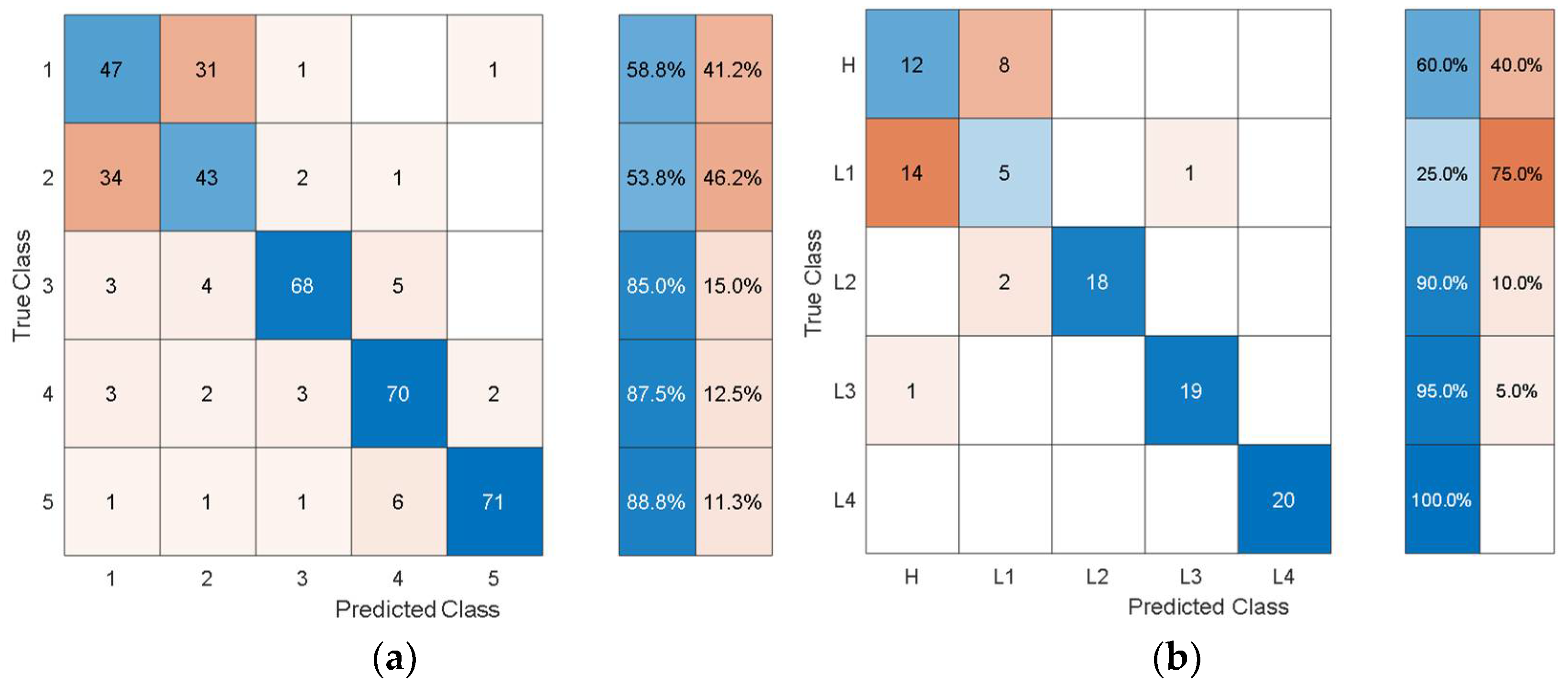
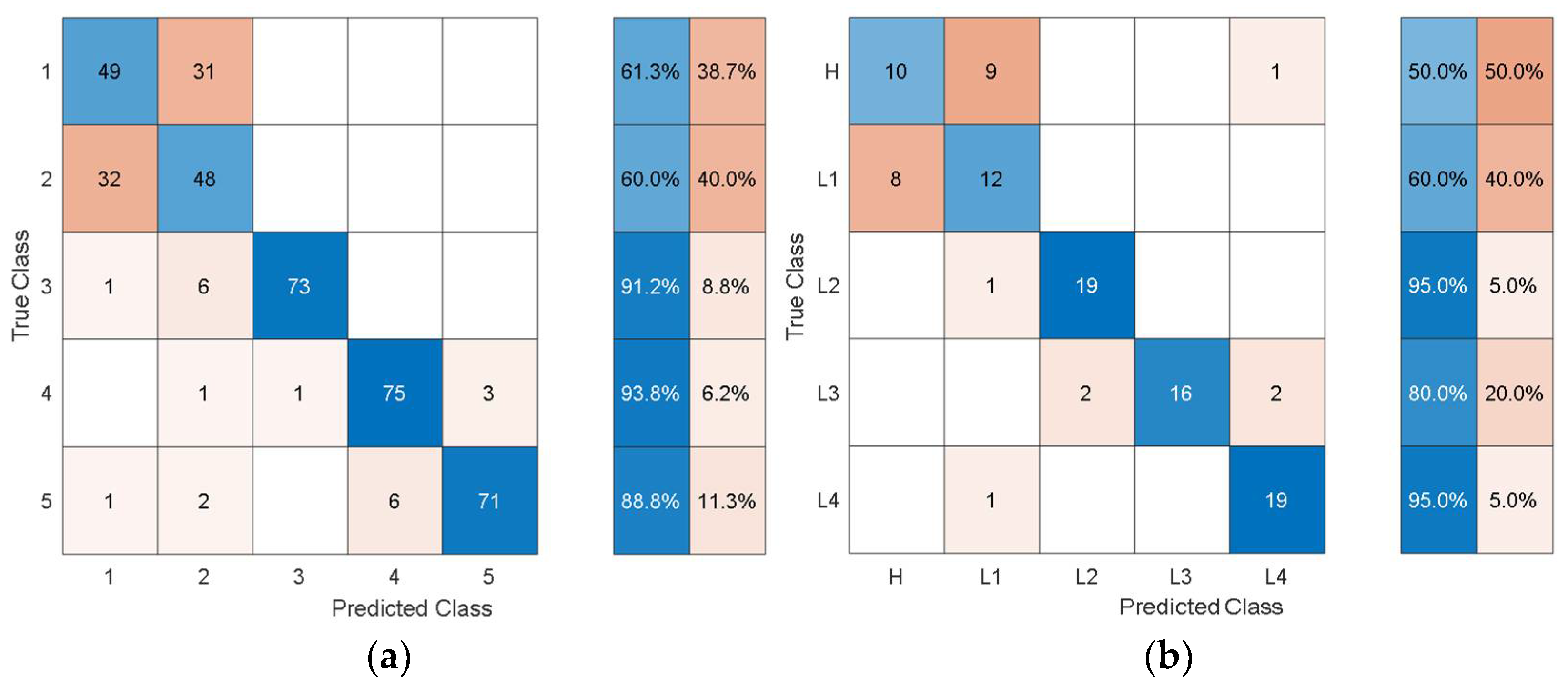
The dataset from the simulation was split into 80% training data and 20% test data. In the confusion matrices, the values on the main diagonals denote correctly classified instances and the off-diagonal cells contain misclassified instances. The blue and red columns on the right depict the recall (true-positive rate) and false-negative rate, respectively, of the actual classes. Quantitatively, the recall gives the successful detection and isolation of a given health state while the false negative gives the susceptibility of a model to confusing other health states with the actual health state. Specifically, from
Figure 9, the autonomous features extracted by Alexnet can distinguish healthy cases H from all other health states with 70% accuracy, but it is susceptible to incorrectly classifying other health states as H at a rate of 30%. The values on the main diagonal and in the off-diagonal cells show that the model is susceptible to the incorrect classification of L1 as H.
From all the confusion matrices, it can be observed that the per-class training performance has substantially increased when using the autonomously extracted features from each of the pretrained models when compared with the training performance using the handcrafted statistical features, as shown in
Figure 6. Moreover, for all the pretrained models, the major losses of accuracy are associated with confusion between the healthy case H and the least severe case of delamination L1. The physical reason for the confusion of H with L1 is that the 3 cm delamination is only causing a very subtle change in the structural stiffness and consequently in the structural dynamic response when compared with the healthy case. The close resemblance in the characteristic dynamic responses of L1 and H causes the classifier to confuse the two cases. Moreover, from the test confusion matrices, it can be observed that the correct prediction rate from using the pretrained model to autonomously extract features, regardless of the model used, is reasonably high and show similar behavior to that shown by the training confusion matrices. The results for the increasing size of delamination and the ease in its detectability in the current work are supported by the research finding of the articles in the references [
50,
53].
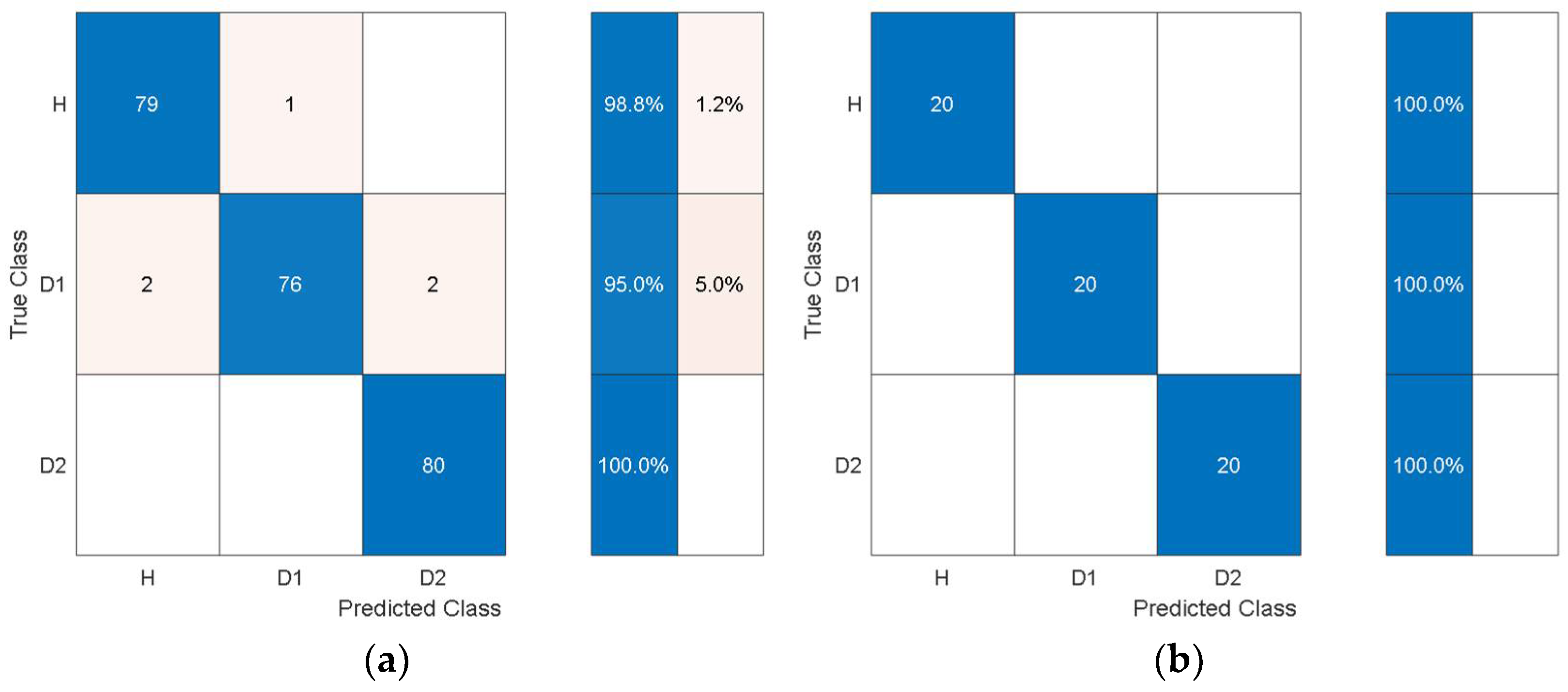
For the experimental data, the structural vibration data windowed into the same smaller chunks used to extract the statistical features from was encoded to time-frequency images using SET. The image data based on the experimental results was processed using pretrained deep learning models to autonomously extract features. The features were extracted through the last layers of the models and were processed with quadratic SVM using 10-fold cross-validation and a one-vs-all training strategy. The experimental data was randomly split into 80% training and 20% test data. The classification results from the SVM using autonomous features are shown in
Table 11.
Comparing
Table 11 with
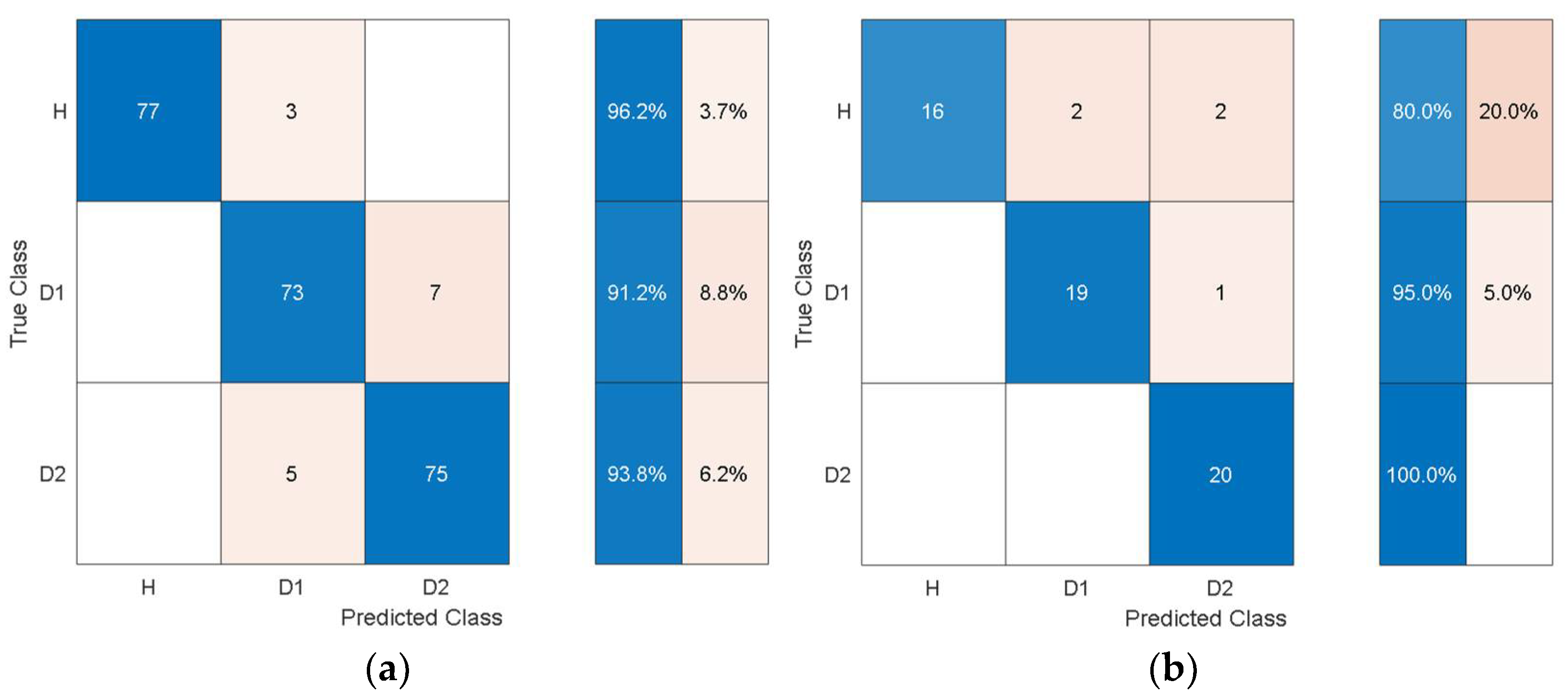
Table 4 shows that the overall training accuracy has substantially increased when using the autonomous features from all the pretrained models. Among the autonomous features extracted by the various pretrained models, the features extracted by AlexNet achieve the best classification performance, while the worst classification performance was observed when using the features from GoogleNet. For a detailed look at the classification performance using features from AlexNet and GoogleNet,
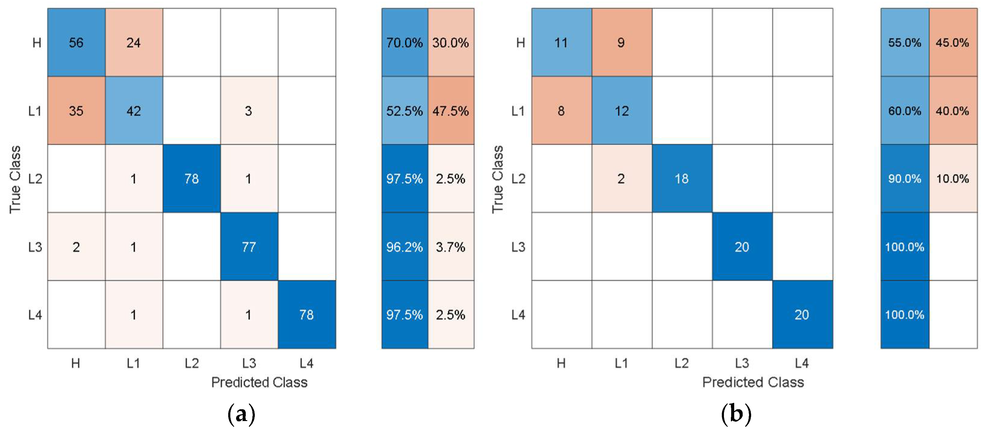
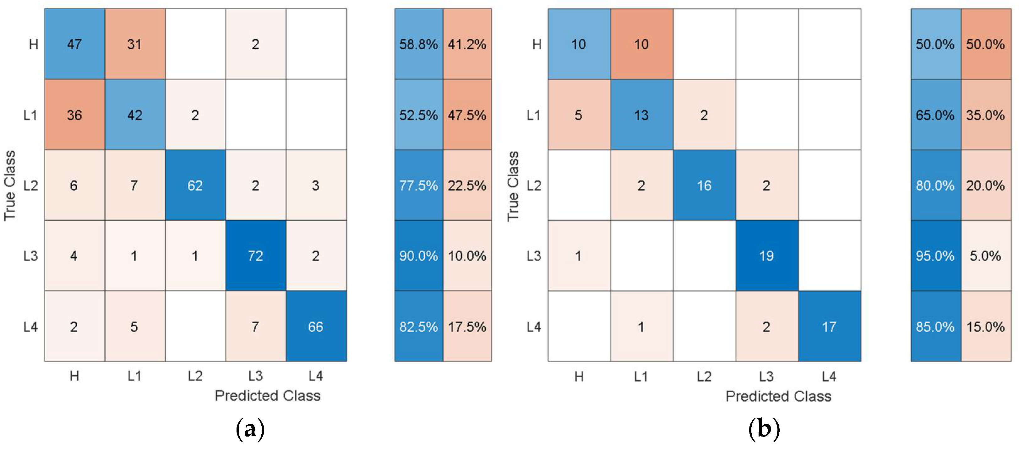
Figure 14 and
Figure 15 show the training and test confusion matrices for the SVM trained on the features extracted by AlexNet and GoogleNet, respectively.
It can be observed that the SVM can distinguish healthy cases from delaminated cases with 98.8% accuracy while it is only susceptible to incorrectly classify other health states as healthy at a rate of 1.2%. The minimum per-class classification accuracy was 95.0% for D1 delamination samples using the features from AlexNet while the maximum per-class classification accuracy was 100% for D2 delamination samples. For the pretrained model with the worst overall classification performance (GoogleNet), the minimum per-class accuracy was 91.2% for D1 delamination samples and the maximum per-class accuracy was 96.2% for the healthy H samples. In general, the autonomous features from all the pretrained models can be used to distinguish between delaminations of the same size occurring at different locations while they can also be used to distinguish healthy cases H from delaminated cases D1 and D2 with higher accuracy. The experimental data has accounted for the uncertainty in the manufacturing of coupons and measurement error by considering five samples of each health state. The existing literature mostly focuses on modal parameters (natural frequencies, modes shapes, mode shape curvature) of structural vibration to assess delamination [
54]. However, modal parameters are global, and the experimental measurement of mode shapes is a difficult task.
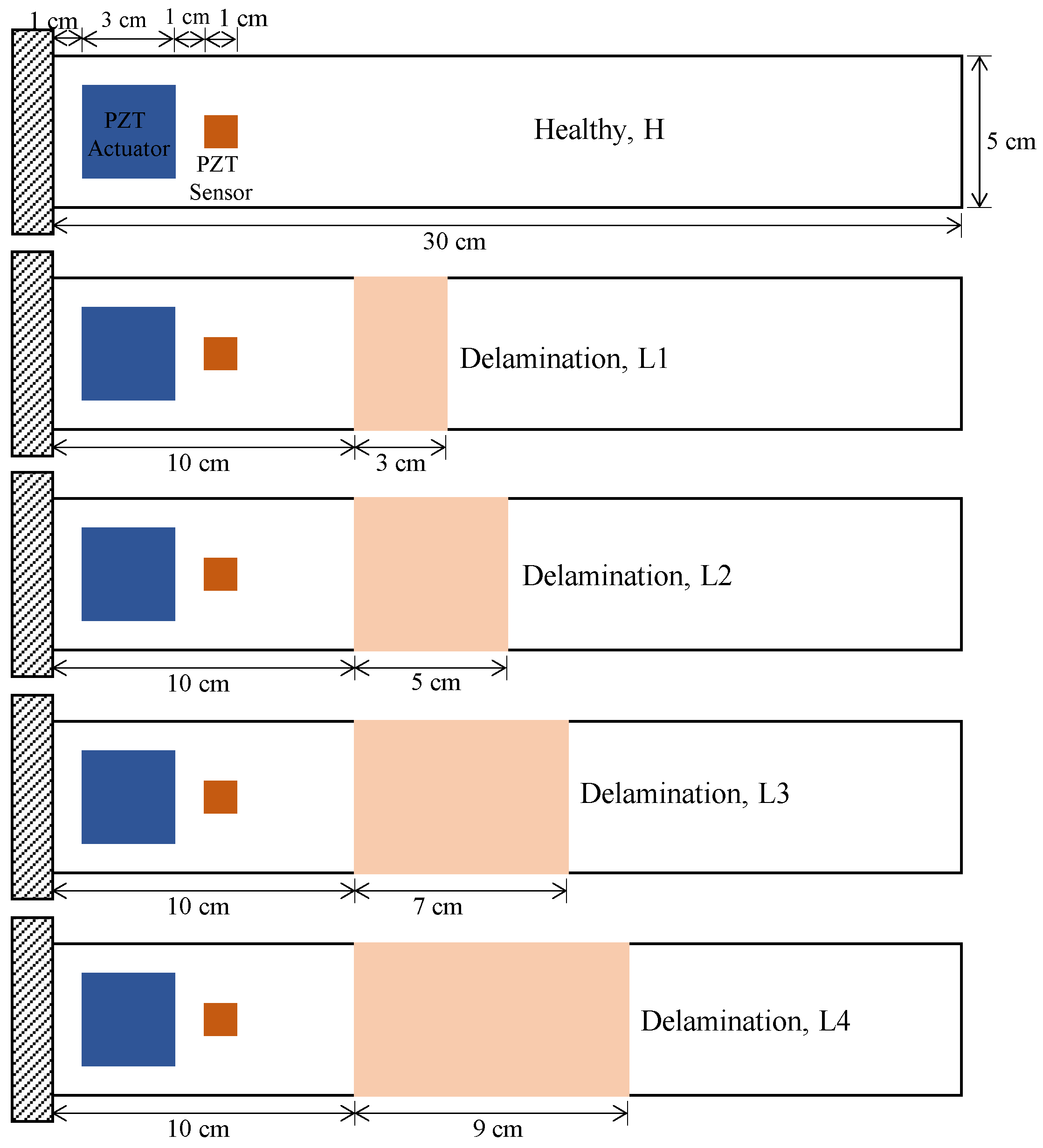
The current work showed the feasibility of limited structural vibration data for the detection, localization, and quantification of delamination through classification in a supervised learning framework. The proposed approach could be employed to assess the size and location of delamination by predicting a label for a given health state which can be interpreted for the size and location of a new delamination. For instance, the label for a delamination of size 6 cm would be either L2 (delamination of 5 cm) or L3 (delamination of 7 cm) due to their similar response characteristics. In general, the delamination of different sizes near the free and clamped ends may have the same dynamics response characteristics, and the new delamination may be entirely different from the one considered in the pretrained model. Moreover, the labels for the prospective delamination may not be known. The future extension of the current work will adopt a more generic approach by using more than one sensor along the length of the specimen and an unsupervised framework for the detection, localization, and quantification of delamination. These results show our approach could be beneficial for delamination localization based on low-frequency structural vibration data.


