4.2. Effect of APCW Size on Network Performance
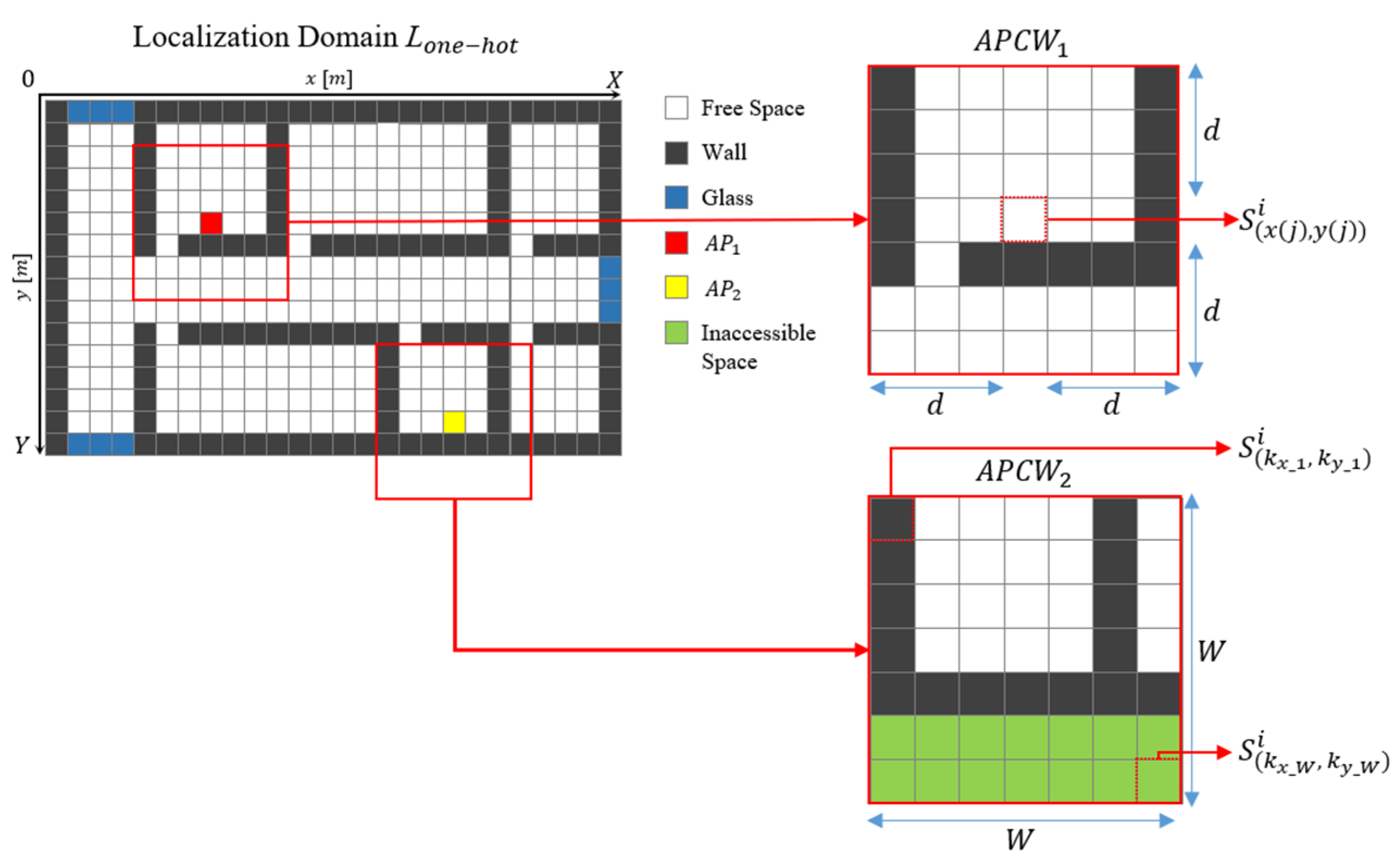
The proposed APCW was generated by partitioning to a certain distance based on the AP location. During this process, if the distance being partitioned was shorter than the propagation distance of the AP, the RGN’s radio-map generation accuracy decreased. However, if the distance being partitioned was longer than the propagation distance of the AP, the RGN’s radio-map generation accuracy increased, because there was sufficient information provided. However, this resulted in increased time spent during RGN training.
In turn, the RGN’s radio-map generation accuracies according to APCW sizes were compared to derive the optimal partitioning distance. APCWs of different sizes were first generated at the same AP location. Subsequently, the generated APCWs were used as input to the RGN to compare the training times for each APCW size.
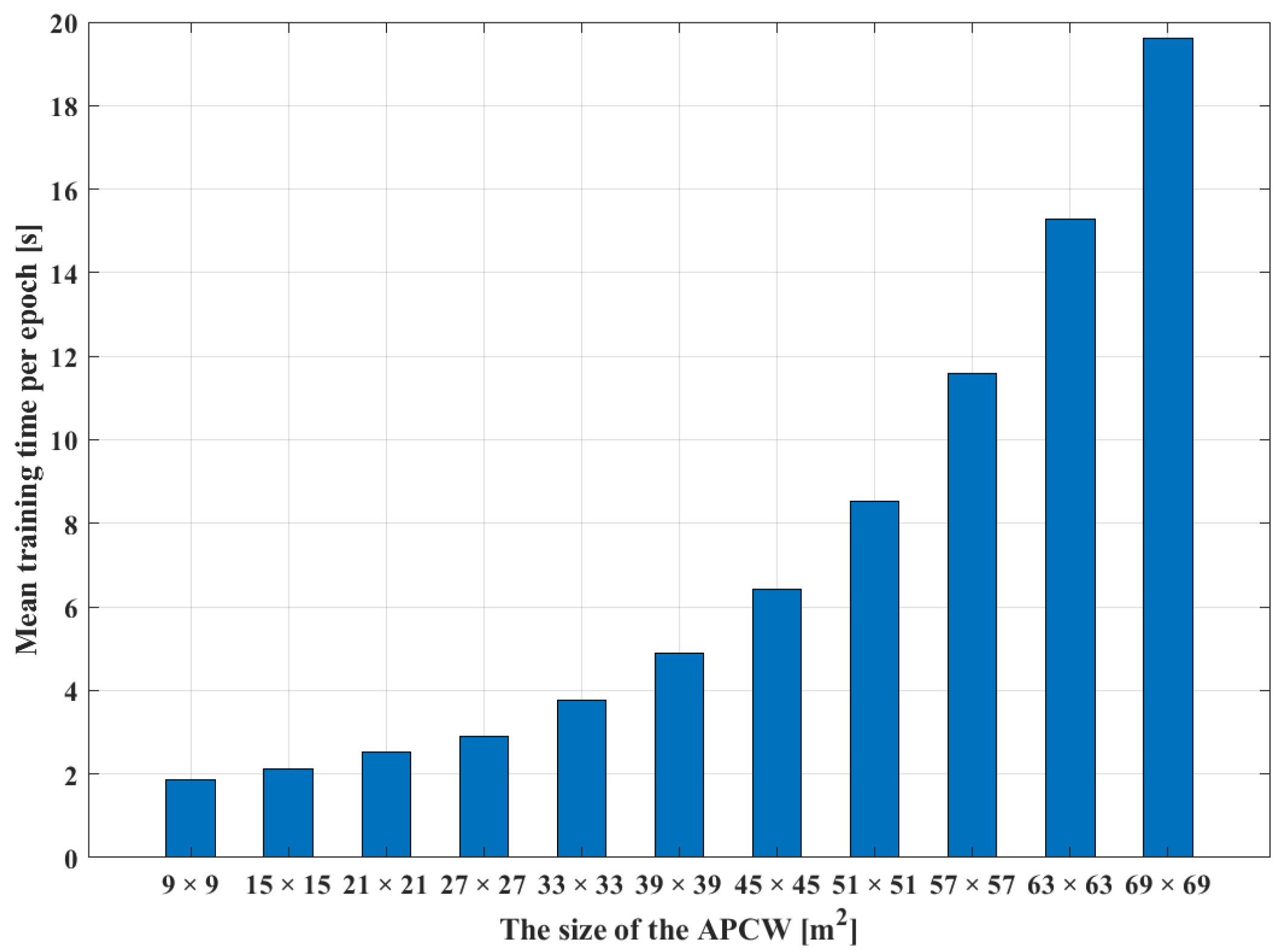
Figure 10 illustrates the training times required per RGN epoch. The results were obtained by increasing the APCW size from
to
. In the figure, the X-axis represents the size of the APCW, and the Y-axis represents the associated training time per epoch. The sizes of the APCWs used as input of the RGN were configured as multiples of
, because each cell of the radio-map generated from the RGN expressed an RSSI of
. Hence, the size of APCW was set to
. As shown in
Figure 10, the training time of the RGN increased in proportion to the square of the APCW size. The training time increased significantly with the size of the collected database. Although both the RGN’s training time and the computational complexity decreased with smaller APCW size, the radio-map generation accuracy also decreased. Thus, it was necessary to consider both the RGN training time and radio-map generation accuracy when selecting the optimal APCW size.
In this study, the RMSE values were calculated using the predicted radio-maps generated from the RGN after using different sizes of APCW and real radio-maps. Then, the RGN’s radio-map generation accuracy was compared according to the size of the APCW.
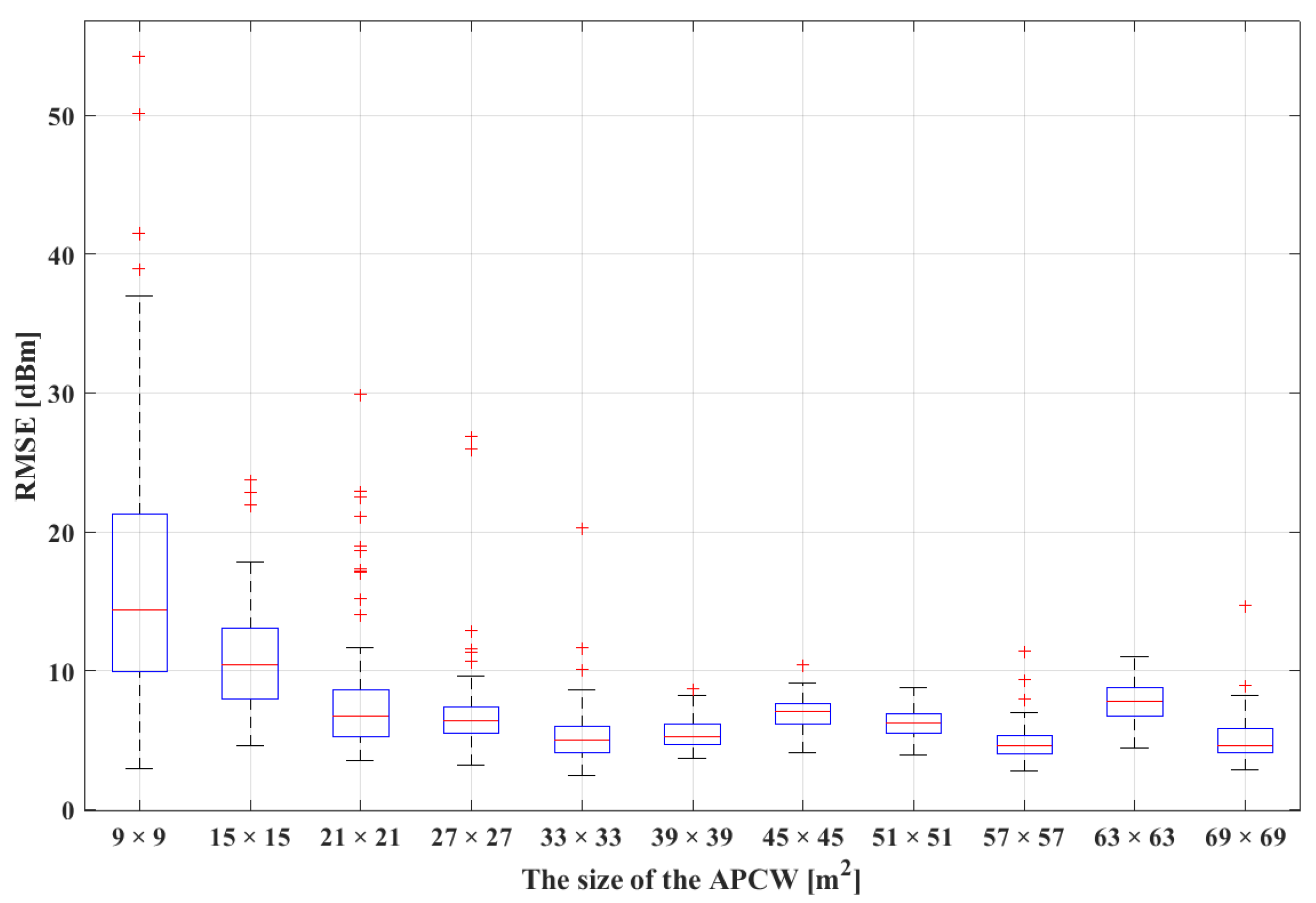
Figure 11 illustrates the distribution of RMSE values in comparison with the predicted and real radio-maps obtained by increasing the APCW size from
to
. In the figure, the
X-axis represents the APCW size, and the
Y-axis represents the RMSE value. To statistically analyze the RGN radio-map generation accuracy, the
Y-axis includes RMSE values of the predicted and real radio-maps calculated based on the AP locations. In the boxplot, a larger box representing the interquartile range (IQR) indicates a lower stability of radio-maps generated by the RGN due to the higher distribution of the RMSE. As the APCW size increased from
to
, the median RMSE value decreased; additionally, the change in the latter was insignificant when the APCW size was larger than
A smaller RMSE value indicates that the predicted radio-map generated by the RGN resembled the real radio-map more closely. An area of
was considered optimal because the median was the smallest among other APCW sizes. However, because the IQR and maximum RMSE were low, an area of
was the most stable RMSE. Additionally, during fingerprinting, the positioning accuracy decreased as the difference between the RSSI distribution collected in real time and the RSSI distribution stored in the radio-map increased. Changes in the RSSI distribution around the AP significantly reduced the positioning accuracy. Therefore, although the lowest median RMSE was obtained when the APCW size was
,
was designated as the optimal APCW size when considering the IQR and maximum RMSE.
4.3. Generation Accuracy and Analysis
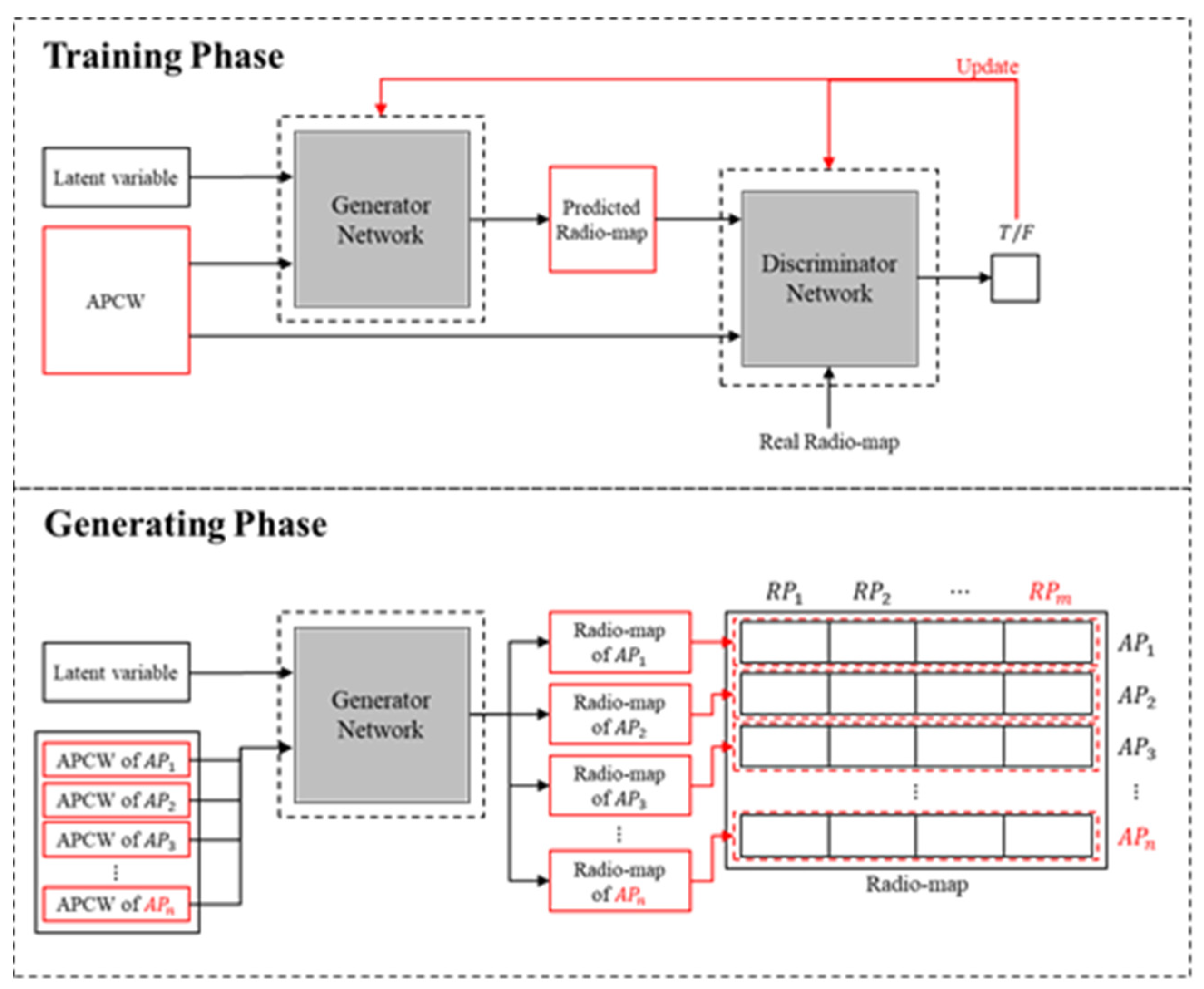
The proposed APCW was generated considering the obstacle types and materials of the indoor space and by removing the radio-shadow areas. Hence, the RGN using the proposed APCW generated accurate radio-maps. Four models using different labels as input were used to analyze the RGN’s radio-map generation accuracy according to the APCW.
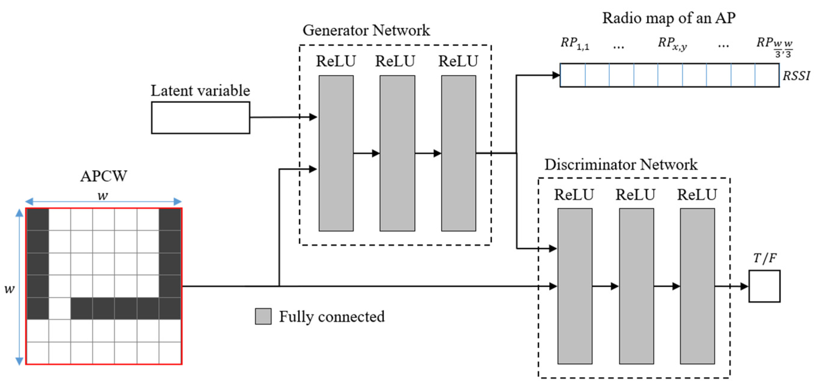
Table 5 summarizes the descriptions, layer (activation function) types, and input and output sizes of the four models designed for the experiment. Model 1 is a basic RGN designed to compare its radio-map generation accuracy to that of the proposed APCW-based RGN, and it uses a label that reflects only the presence of obstacles as input, such as in [
27,
30]. Model 2 is an RGN model that uses a label reflecting only the material of obstacles as input. Model 3 uses a label based on the AP location while reflecting the presence of obstacles. Model 4 is the proposed APCW-based RGN that uses labels generated based on the AP location while reflecting the obstacle materials.
In the table,
denotes the latent variable;
X denotes the size of the building along the
X-axis;
Y denotes the size of the building along the
Y-axis;
denotes the size of APCW; and
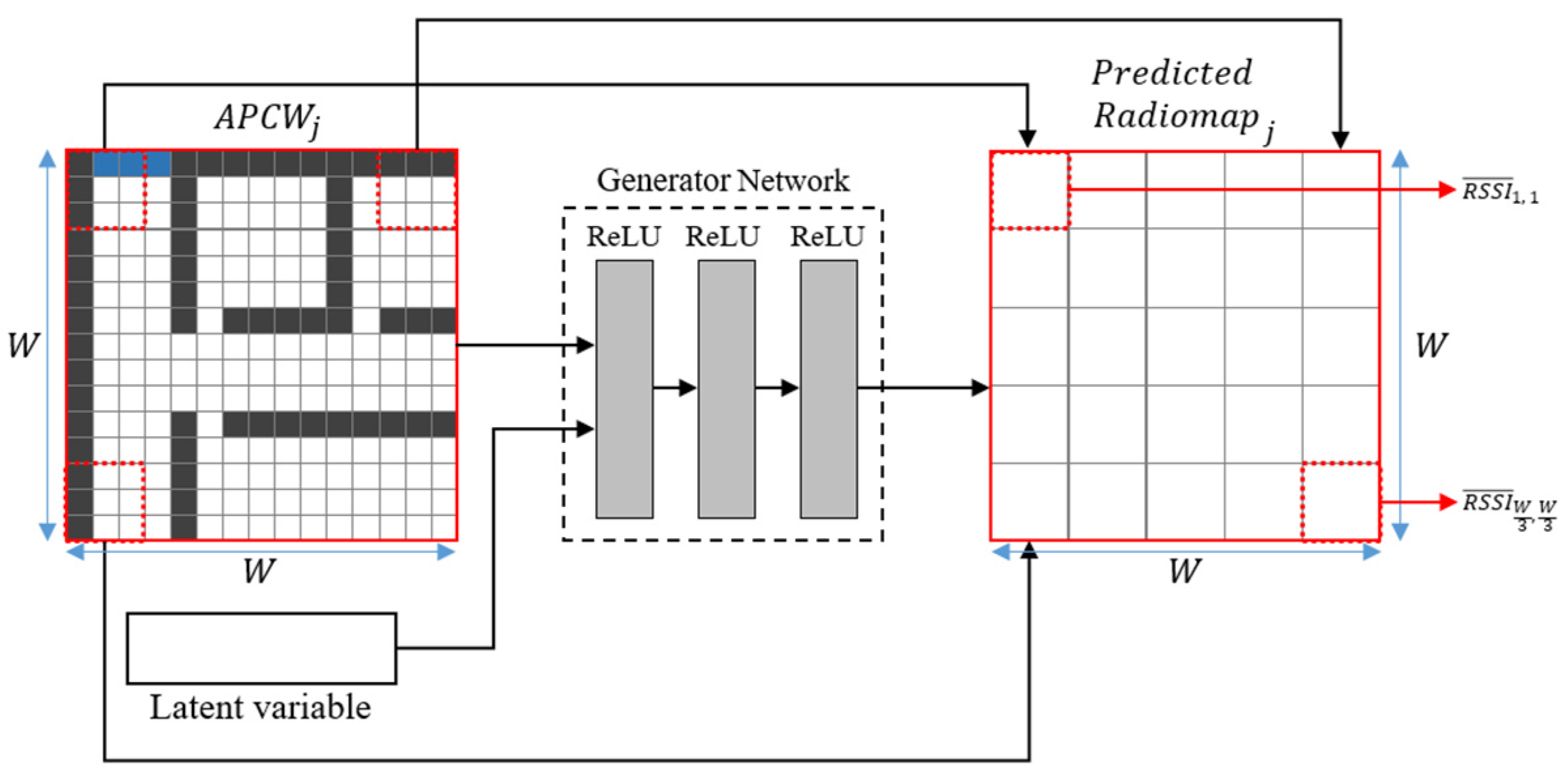
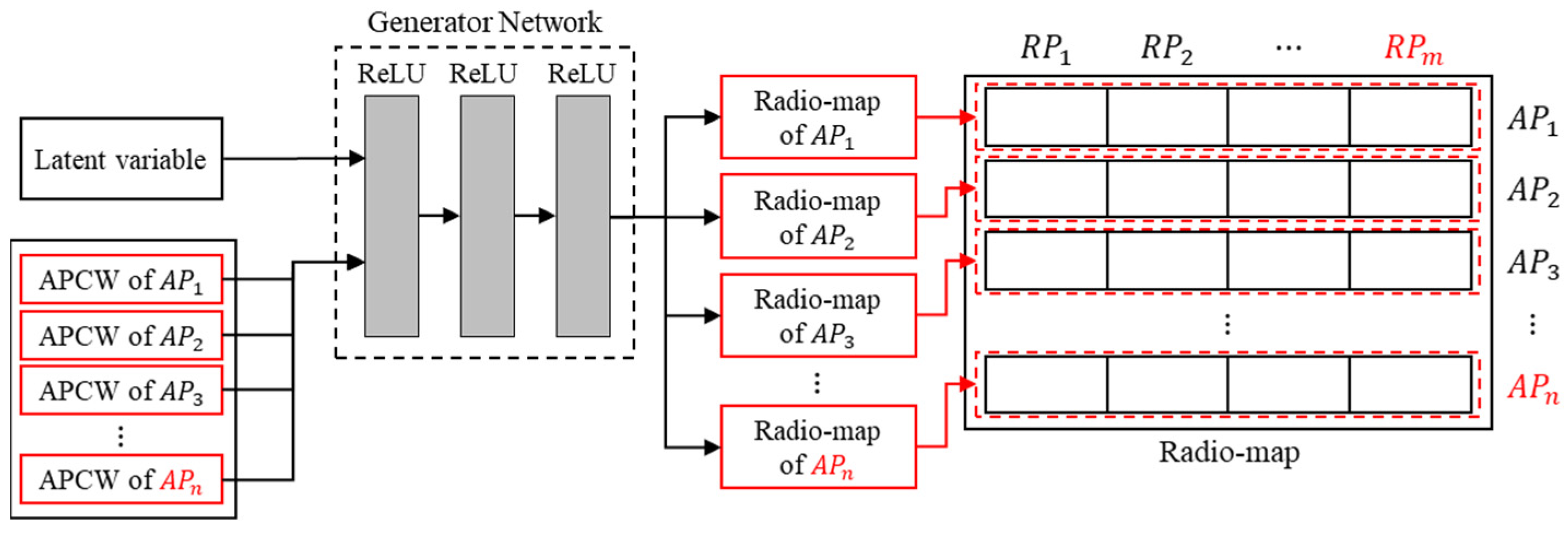
denotes the number of indices. The generator was designed to receive a latent variable and a
label while generating a
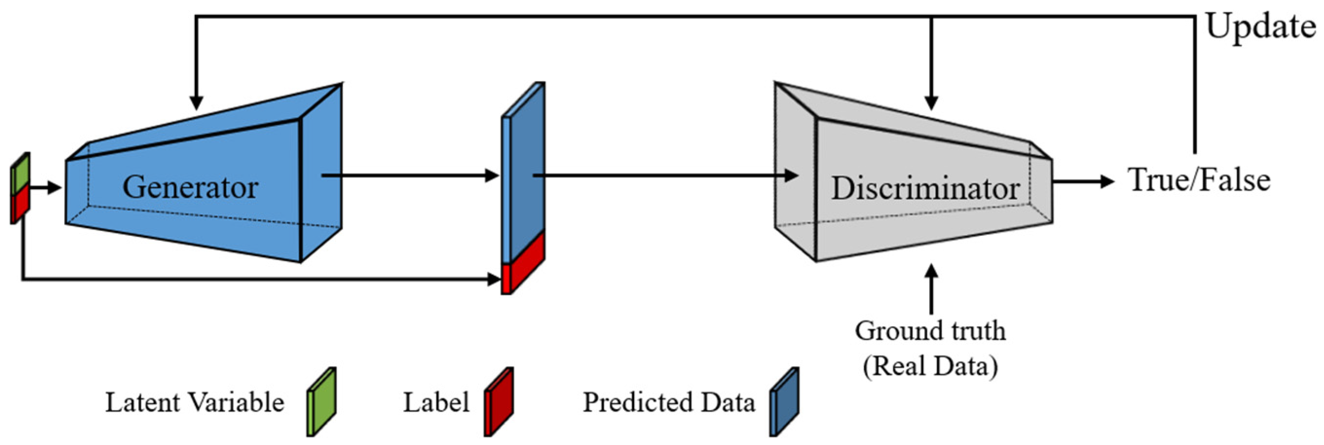
predicted radio-map. Additionally, the discriminator receives the predicted radio-map generated by the generator alongside the label to determine whether the received predicted radio-map is identical to the real one. Because the input and output sizes of the generator and discriminator comprising each model were determined based on the size of the label, the input and output shapes of
Table 4 are as follows. The label size of
used as the input to Models 1 and 2 was set as
in accordance with the shape and size of the building. Furthermore, the label size of
used as the input of Models 3 and 4 was set as
, which provides the optimal RGN radio-map generation accuracy according to the experiment results from
Section 4.2. Meanwhile, the vanishing gradient problem can still be experienced because the generator and discriminator of each model comprise three layers each. To address this problem, ReLU was used as the activation function [
42].
The
Table 6 shows the network sizes of generators and discriminators according to each model. the size of the model changes according to the input structure of each model. When comparing Models 2 and 4, the size of the models shows a significant difference of about three times. When generating a radio-map, as the distance from the AP is increased, the distribution of the RSSI signal needs to be learned even in a space where the signal-to-noise ratio increases, so the radio-map generation accuracy can be reduced. In addition, floor plan-based RGN predicts not only the location that can receive the signal from the installed AP, but also the location where it will not receive the signal, so unnecessary computation is increased. On the other hand, since APCW-based RGN divides the radio-map prediction space into constant windows centering on the AP, it is possible to reduce the amount of unnecessary computation in the radio-map.
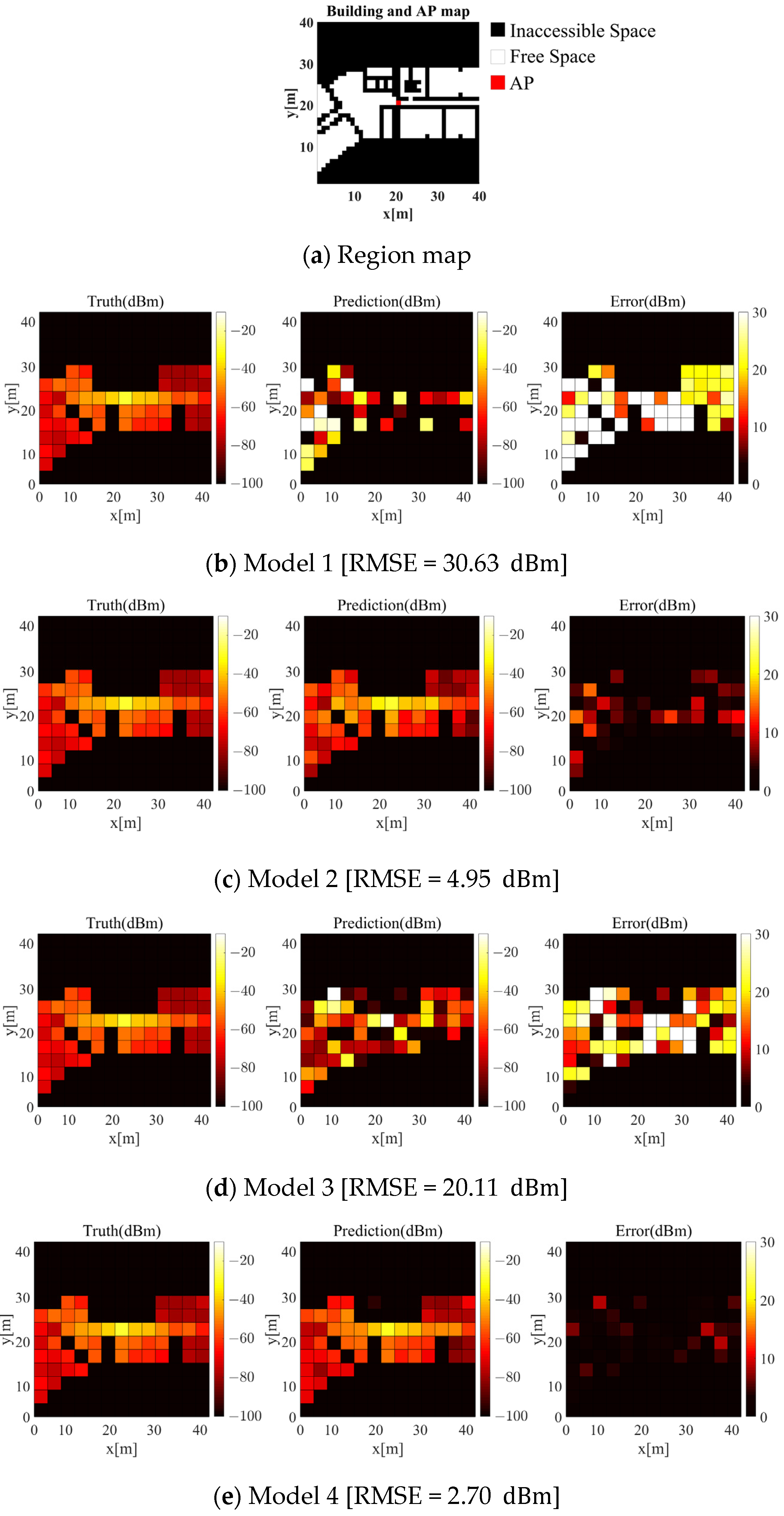
Figure 12 illustrates each model’s radio-maps generated by predicting the signals emitted from one AP.
Figure 12a displays region maps to compare the generation accuracy of each model. In
Figure 12a, red cells indicate the AP location; white cells indicate free space; and black cells indicate inaccessible space. Images in
Figure 12b–e display the radio-map generation results obtained by Models 1, 2, 3, and 4. Models 1 and 2 generated
sized radio-maps using a label that converted an entire building map into data, whereas Models 3 and 4 generated
sized radio-maps. Hence, the size of the region-map used to compare the radio-map generation accuracy of each model was configured to
, as with the output size of Models 3 and 4.
When comparing the results obtained by Models 1 and 2 and Models 3 and 4, it can be seen that the radio-map generation accuracy significantly increased when the obstacle materials were considered. This indicates that Models 2 and 4 learned that the degree of RSSI signal reduction from the AP differed according to the materials of obstacles (e.g., steel frame and concrete). In turn, the models predicted accurate radio-maps. Furthermore, as shown from the results of Model 4, which reflects both obstacle material and AP location, a high accuracy of radio-map generation was obtained at the center area adjacent to the AP. Accurate prediction of the radio-map of the area adjacent to the AP is important when maintaining the stable positioning accuracy of fingerprinting. As such, the advantages of Model 4 can be maximized, because it enables accurate prediction of the radio-map of the area adjacent to the AP. Images of
Figure 12 represent radio-maps generated for one AP location point, and the accuracy can vary depending on the AP location. Therefore, to quantitively evaluate the radio-map generation accuracy of each model, radio-maps were generated for 110 different AP install locations, and RMSE values were derived.
Table 7 displays the average, maximum, and minimum RMSE values obtained. As shown from the results of Models 1 and 3, the average RMSE value improved from 28.84 to 14.98 dBm when the label reflecting the AP location was used. Generally, a Wi-Fi signal has a standard deviation of ~0–5
[
45]. Accordingly, the radio-maps generated by Model 3 cannot be applied to fingerprinting, because the positioning accuracy is lower, owing to outliers. Thus, Model 3, which considers only the AP location, is unsuitable. Therefore, the radio-map generated by Model 3 considering only the location of the AP showed higher performance than did Model 1, because it learned the pattern of radio waves radiated to the AP location. When comparing the results of Models 1 and 2, the average RMSE significantly improved from 28.84 to 5.48
when the label reflecting only the obstacle material was used. Thus, it can be inferred that the accuracy of RGN’s radio-map generation can be significantly improved, even when considering only the obstacle materials.
Lastly, when comparing the results of Models 2 and 4, the accuracy of the RGN radio-map generation improved from 5.48 to 4.01
when both the obstacle material and AP location were considered. As described in
Table 5, Model 1 and Model 2 use the entire floor plan without dividing the window through APCW. The reason for this is that the loss function is learned not only in the close range of the AP, but also in the range that is difficult to predict, so the radio-map generation performance is comparatively lower than that of Models 3 and 4. Therefore, performance is improved by limiting the range away from the AP through APCW. Accordingly, highest radio-map generation accuracy was obtained when the proposed APCW was used as input to the RGN, and the average RMSE value was ~4 dBm, showing stable performance. As a result, Model 4 is the optimal RGN.
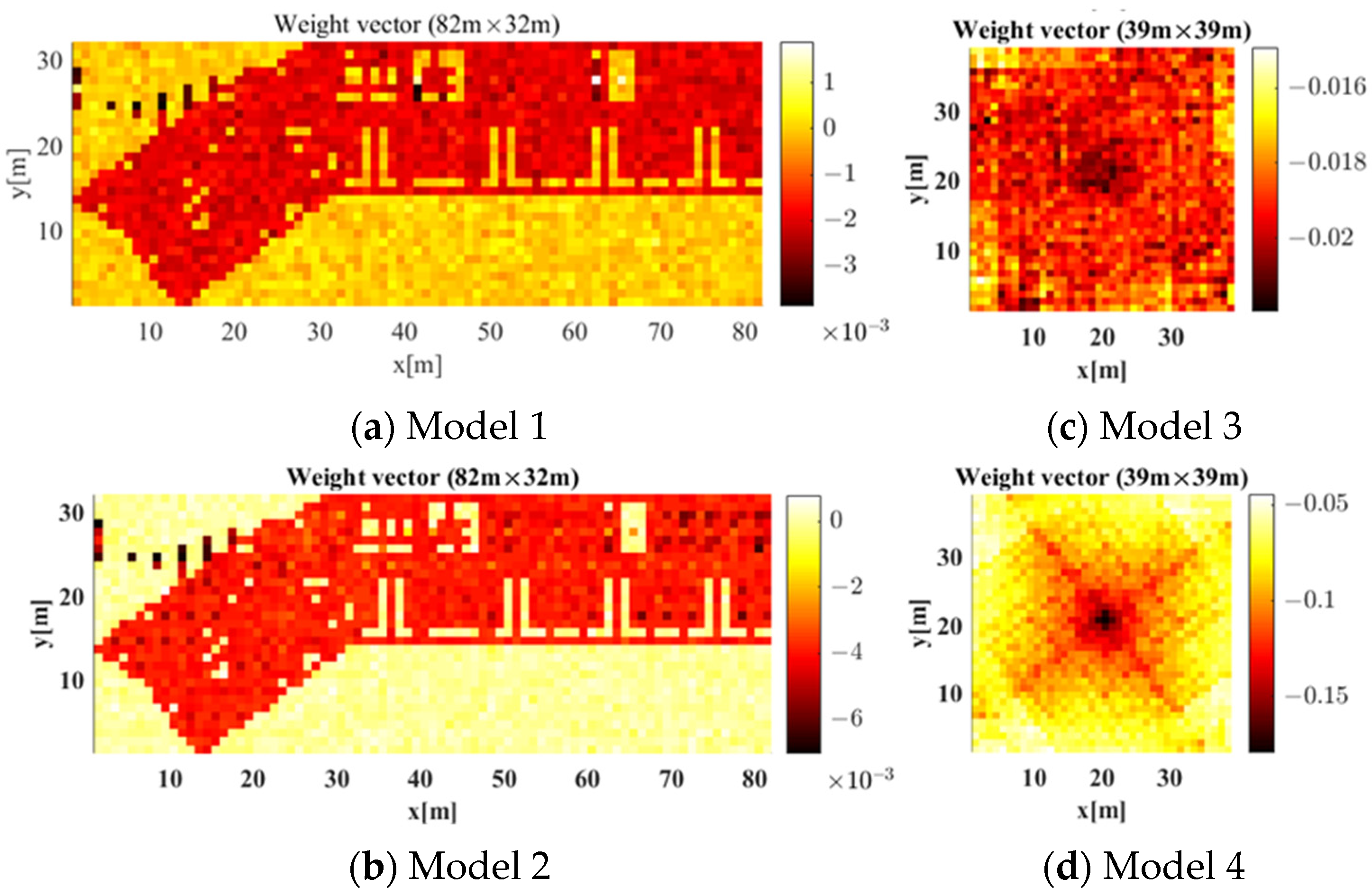
The radio-map generation accuracy was enhanced when the label reflected both obstacle material and AP location rather than only the material. The weight vectors constituting the input layers of Models 1 to 4 were compared to analyze the factors affecting radio-map generation accuracy.
Figure 13 displays the weight vectors constituting the input layers of Models 1 to 4. In
Figure 13a,b,
X and
Y axes represent
X and
Y coordinates of the weights constituting the weight vectors of Model 1 and 2. Here, the size and shape of the label were configured to be same as the size of the building. Additionally, in
Figure 13c,d,
X and
Y axes represent
X and
Y coordinates of the weights constituting the weight vectors of Model 3 and 4. Here, the size and shape of the APCW were set as
(i.e., the size yielding the most stable radio-map generation accuracy of RGN based on the experiment results from earlier section). When data were entered into a typical network, each component constituting the data and the weight vector of the input layer were multiplied. Then, all multiplied values were added and sent to the subsequent layer. Thus, the weights for each location in the weight vector indicate the ratio of components used at the corresponding location in the input data to derive output results for the network.
As shown in the results of Model 1 and 2 in
Figure 13a,b, the weight vectors were learned using the shape of the building as input, and the weights had similar values regardless of location, except for inaccessible spaces. Based on this, Model 1 and 2 used each component constituting the label similarly regardless of the distance between the component and the AP location when generating a radio-map. The signal strength emitted from the AP decreased as the distance from the AP increased, owing to path loss. This results in a radio-shadow area. However, Model 1 and 2, which show similar weights regardless of location, do not reflect a radio-shadow area. Thus, they cannot generate an accurate radio-map.
On the other hand, as shown in the results of Model 3 and 4 in
Figure 13c,d, the weight vectors had the highest values at the center, which gradually decreased as the distance increased from the center. For signals, propagation phenomena (e.g., reflection and diffraction) occurred with obstacles, including walls, and the radio-map distribution changed, owing to the propagation phenomenon becoming smaller as the signal strength decreased. Accordingly, the radio-map distribution change became smaller with the increase of the distance between the AP and the obstacle.
Although the experimental environment does not resemble a perfect propagation pattern, because it used an indoor environment with various obstacles, Model 4 can more accurately learn these propagation characteristics than Model 3. Therefore, Model 4, which uses an APCW-based RGN to reflect both radio-shadow areas and propagation characteristics, enables the generation of accurate radio-maps.
To analyze whether the RGN that learned the indoor structural patterns generated accurate radio-maps, an experiment was conducted to compare the RGN accuracy per AP location.
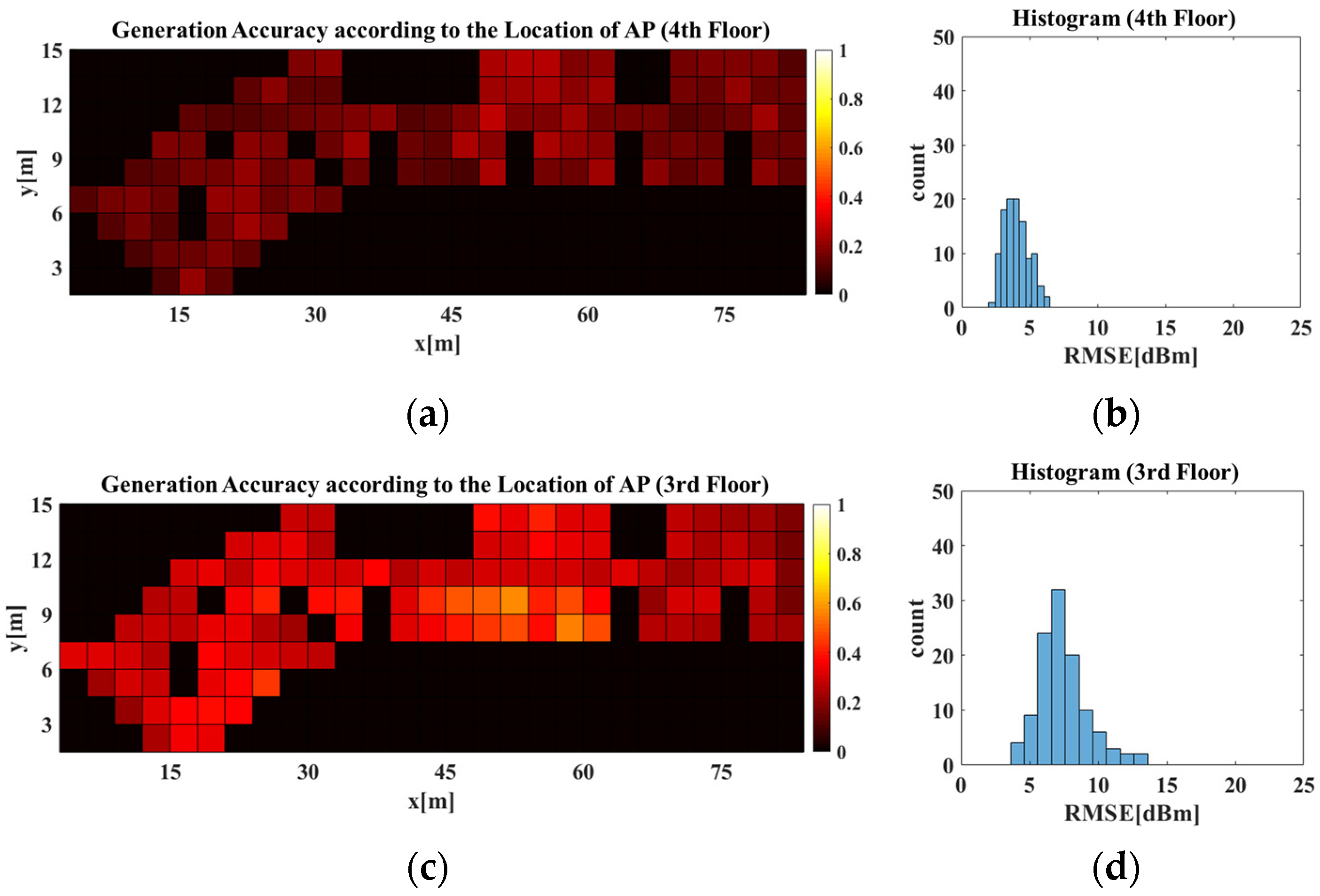
Figure 14 displays radio-map generation accuracies obtained from different AP locations on the 3rd and 4th floors using the RGN trained with data collected from the 4th floor. In
Figure 14a,c, RMSE values between the predicted radio-map generated by the RGN when the AP were located at arbitrary
X and
Y coordinates in
, and the real radio-map of the corresponding AP location was displayed. Here,
X and
Y axes represent the coordinates of the AP location. Each cell shows the result of the RMSE of real vs. predicted RSSI in RPs according to the location of the AP, and the darker the color of each cell, the lower the error of predicted RSSI at the coordinates of the AP location.
Figure 14b,d each show histograms of
Figure 14a,c, respectively. A histogram expresses the size of components comprising the data and the frequency distribution of such sizes. Because there was difficulty checking results of individual cases, owing to the substantial number of APs and RPs in the experiments, histograms were used to statistically analyze the results. A smaller RMSE value indicates a higher radio-map generation accuracy. Thus, having a higher distribution on the left side of the RMSE histogram indicates higher radio-map generation accuracy. In the histogram, the
X-axis represents the RMSE value between the predicted and real radio-maps, whereas the
Y-axis represents the frequency of the values. As shown in the results of
Figure 14a,b, the RGN generated an accurate radio-map regardless of the AP location on the 4th floor. This indicates that the RGN generated the radio-map after learning the structural patterns of the APCWs, which change per AP location and the radio-map distributions of the corresponding structures. For the results of
Figure 14c,d, the RGN’s radio-map generation accuracy decreased on the 3rd floor compared with 4th floor when the AP was positioned at the center. This can be attributed to the structural difference at the center and the lower-left parts of the floors. Extant methods were limited to specific buildings used for training, but the proposed APCW-based RGN enables radio-map generation without measuring Wi-Fi signals, even when applied to new buildings. Thus, radio-maps were generated that learn all 3rd and 4th floor structures.
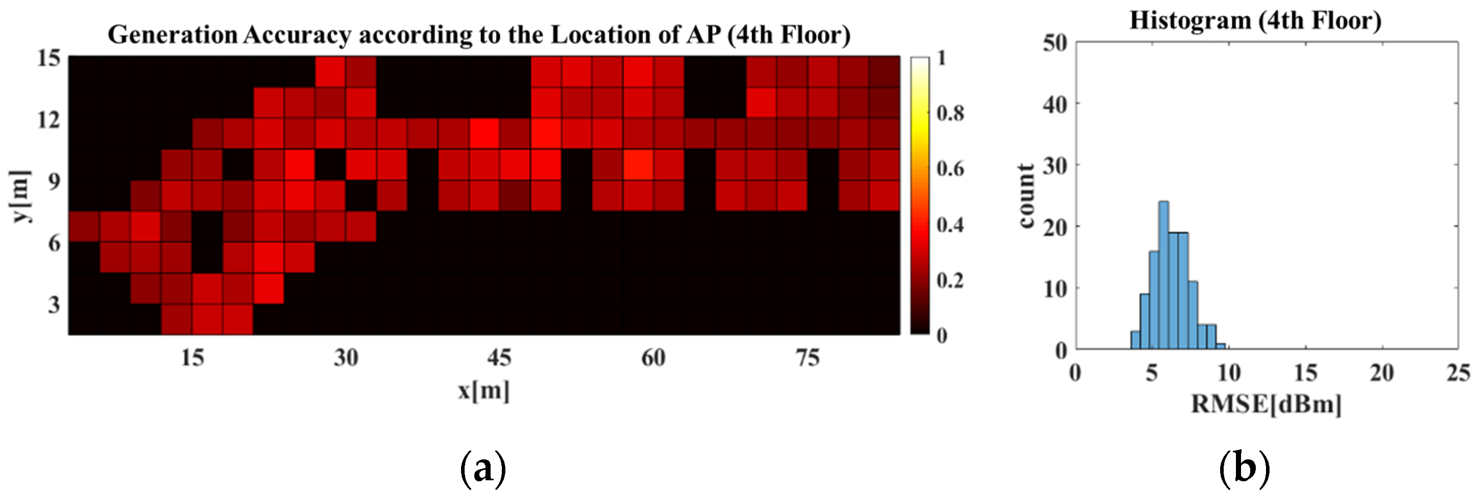
Figure 15 displays the radio-map generation accuracy for the 3rd and 4th floors obtained using the RGN trained with data collected from 3rd and 4th floor dataset. where X and Y axes in the images of
Figure 15a–d were the same as in the images of
Figure 14a–d. As shown in
Figure 15c,d, the RGN trained using data from both floors generated a more accurate radio-map compared with the RGN trained with data of only the 4th floor. This indicates that the APCW-based RGN learned patterns of new structures and generated a good radio-map.
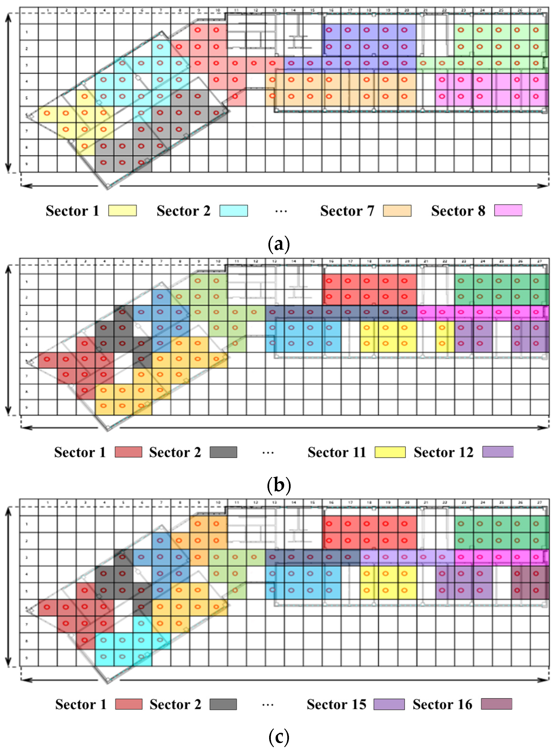
We compared the localization accuracy using the radio-map generated by the proposed RGN and that measured by the walking survey. We used a radio-map constructed by randomly arranging APs to compare the localization accuracy according to the number of APs. The number of APs used was divided into 8, 12, 16, and 20 parts in consideration of the building environment.
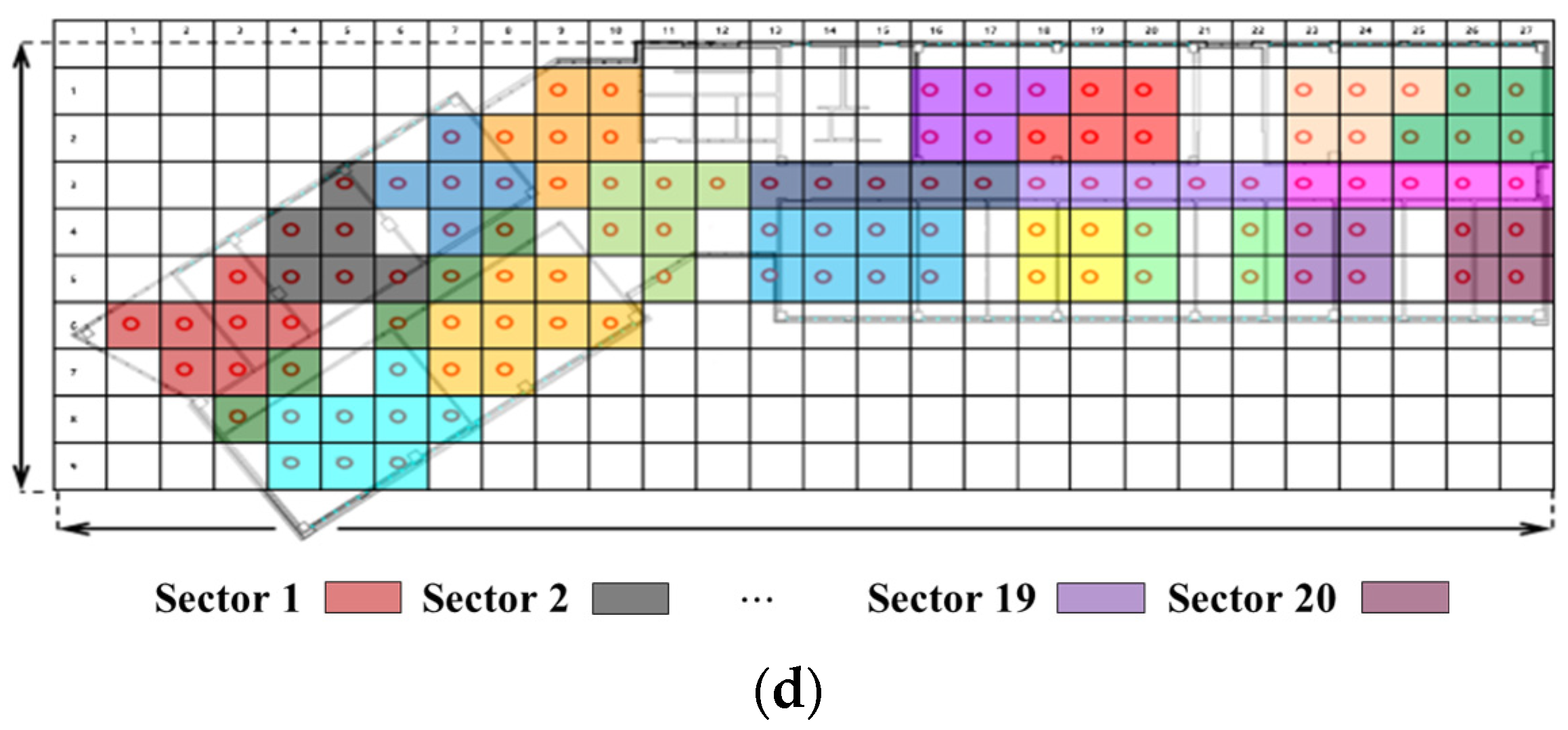
We divided the region map into sectors according to the number of APs to enable localization of all RPs.
Figure 16 shows the sectors placed divided according to the number of APs in the region map of the localization experiment environment. We randomly selected one AP for each sector to compare and analyze localization performance. As for the experimental RSSI data, the RSSI data measured 200 times for each AP in RP were randomly sampled and converted to 250 for each RP, and the total number used in the experiment was 27,500.
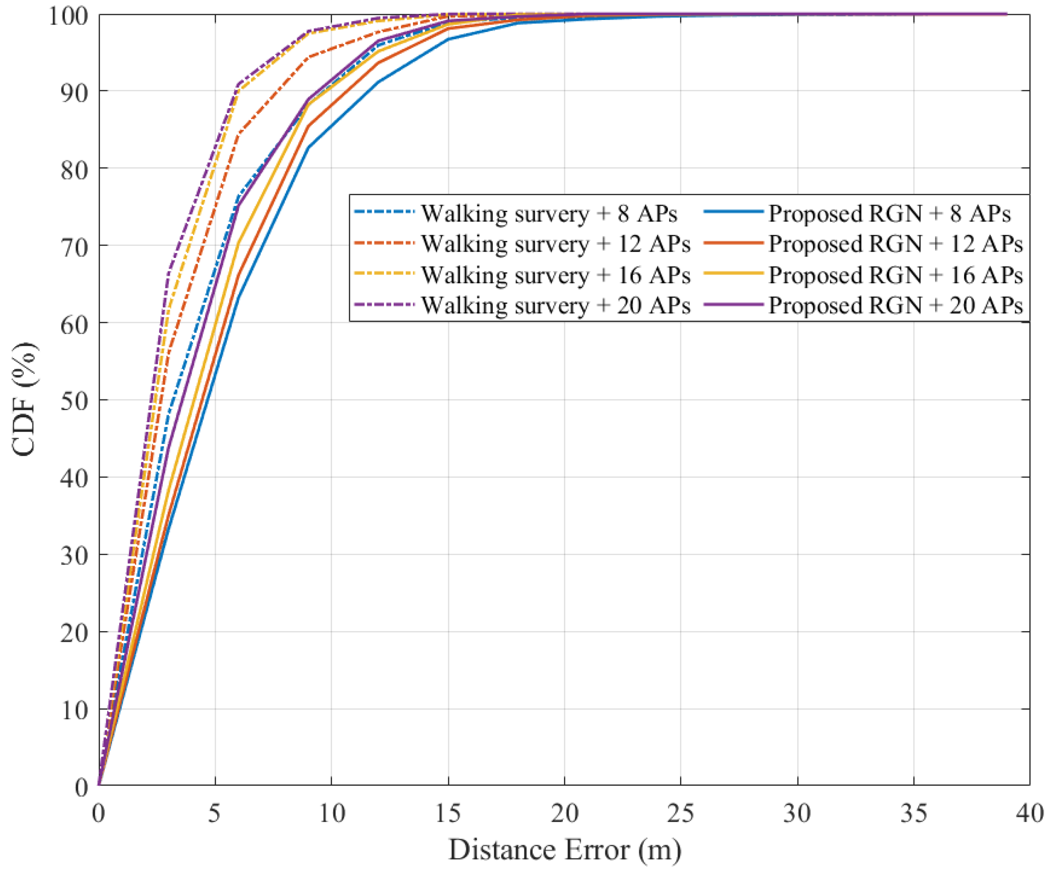
Figure 17 shows the result of localization errors based on the radio-map constructed using the walking survey and the RGN in the cumulative distribution function (CDF) graph. There was a difference in performance according to the number of APs. As the number of installed APs increased from 8 to 20, the localization error decreased from 2.13 to 1.23 m in the walking survey and from 4.79 to 3.34 m in the proposed RGN. In the CDF graph, it can be seen that the walking survey using eight APs and the RGN performance using 20 APs were slightly different.
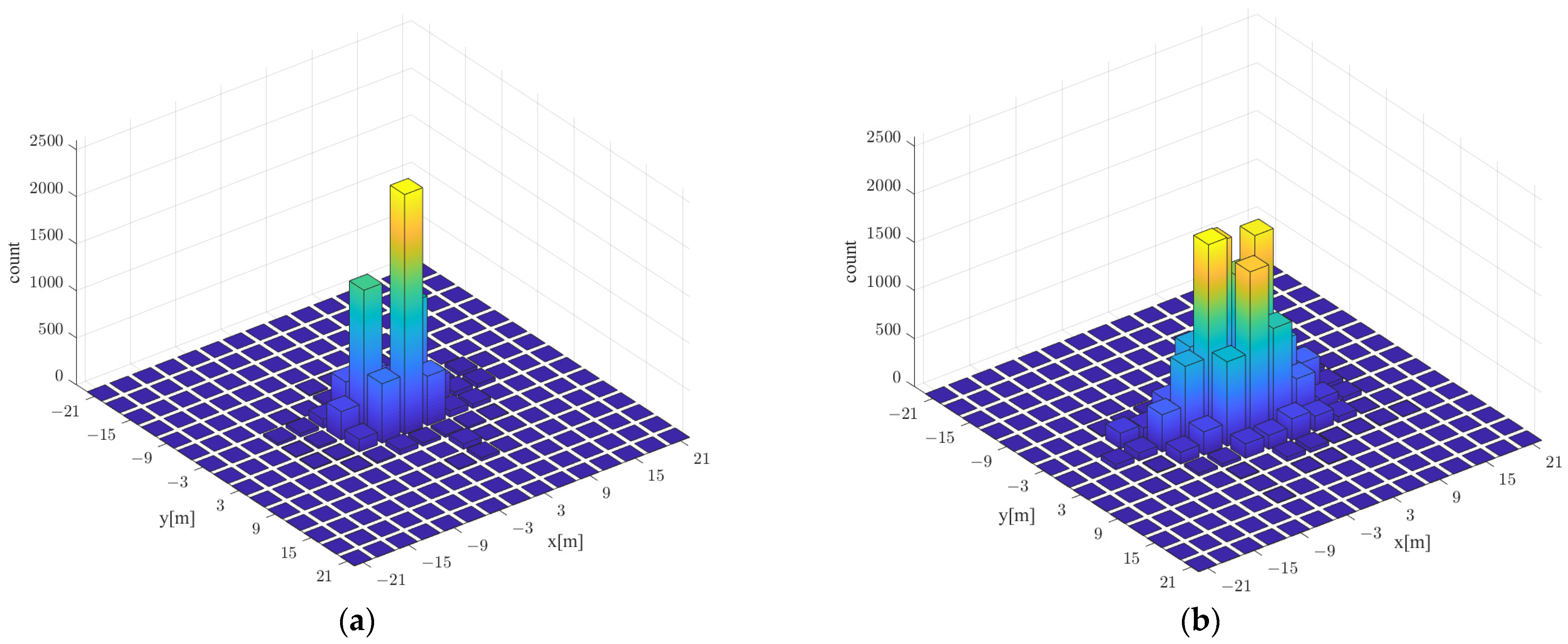
Figure 18 shows the error distribution of real and predicted locations using walking survey and proposed RGN-based localization. The
x-axis and
y-axis represent the error location of each axis, and the z-axis represents the frequency according to the error of each predicted location. In this experiment, localization was performed 27,500 times using the experimental data randomly sampled 250 times among the RSSI data measured 200 times per AP at 110 locations in the environment shown in
Figure 15d. The distribution of localization errors based on the walking survey shows that the maximum frequency was 2550 at the point where the
y-axis was 3 m apart, which is biased compared with other points. The distribution of the proposed RGN-based localization errors was the maximum frequency of 1967, which showed a balanced form according to the direction. The two approaches had significant differences in localization performance, but the radio-map generated using the proposed RGN only required information on the floor plan, and the radio-map constructed using the walking survey required RSSI of each AP collected with 200 repetitions per RP. In other words, by implicitly inferring radio-map using the proposed RGN, there was an advantage of reducing collection times and workloads.
