
Integrated Pose Estimation Using 2D Lidar and INS Based on Hybrid Scan Matching

Abstract
1. Introduction
2. Related Work
- (1)
- Develops classification and integration mechanism with different point clouds, allowing both point-to-point and point-to-distribution based scan matching.
- (2)
- Adapts the uncertainty of feature points into the pose optimization scheme.
- (3)
- Presents localization accuracy in the real world through INS integration.
- (4)
- Validates the proposed algorithm through the results of the reference method from both simulation and experiments.
3. Algorithm Implementation
3.1. NDT Formulation
3.2. NDT-P2P
| Algorithm 1. Register scan pointsto mapusing NDT-P2P |
| NDT-P2P |
| 1: { Initialization : } same as NDT in Reference [11] 2: { Points Extraction : } 3: Allocate feature group structure 4: Extract feature points that contains 5: Store feature points in feature group 6: if feature group size > window size j do 7: Remove a j-th prior feature point in feature group 8: end if 9: for all feature group do 10: all feature points within i-th group 11: 12: 13: end for 14: { Registration : } 15: While not converged do 16: 17: 18: 19: for all points do 20: if is feature points do 21: find the closest point from 22: else 23: find the cell that contains 24: end if 25: score (see Equation (12)) 26: update 27: update 28: end for 29: solve 30: 31: end while |
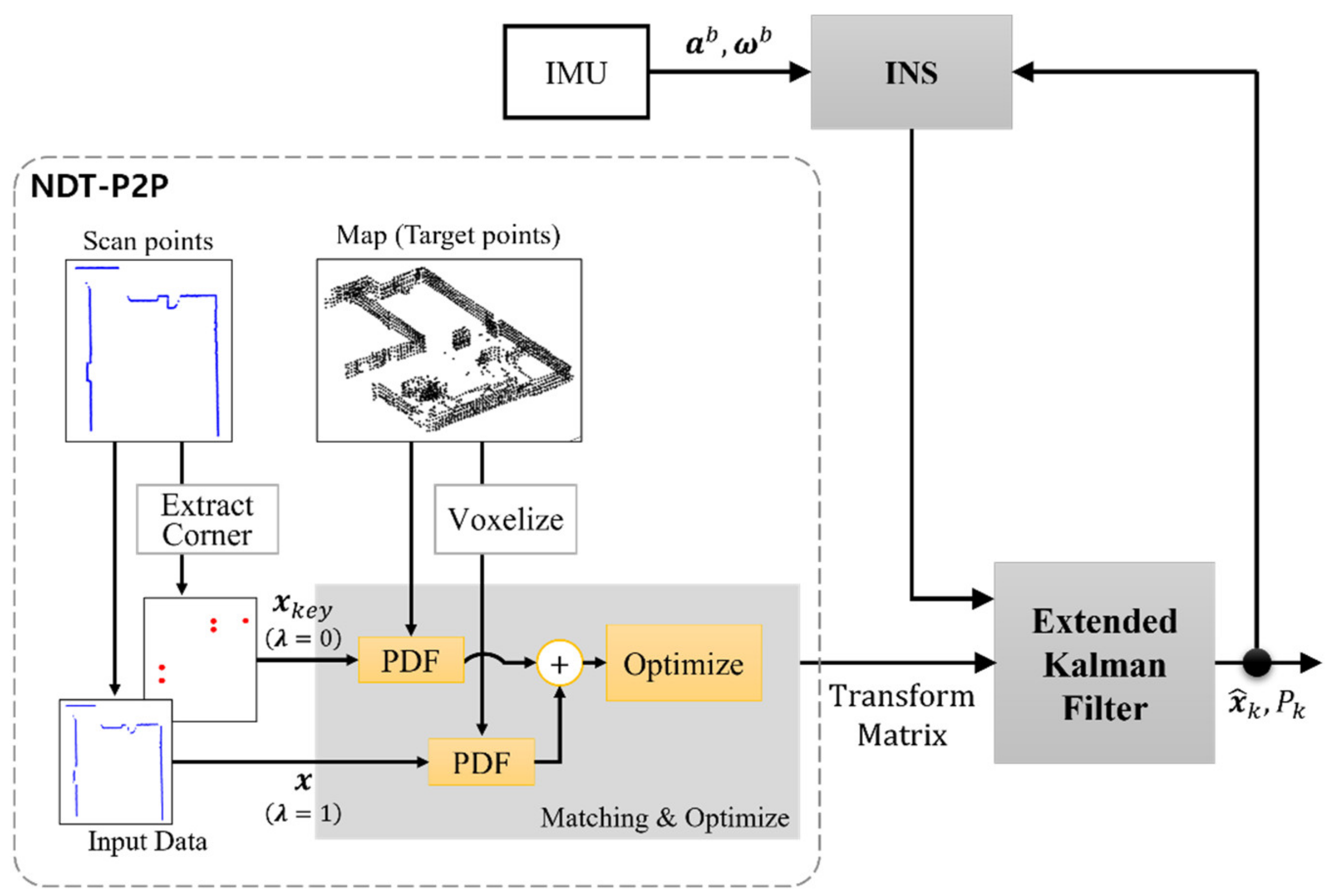
3.3. INS Integration
4. Simulation and Experiment
4.1. Simulation
4.2. Experiment
5. Conclusions
Author Contributions
Funding
Institutional Review Board Statement
Informed Consent Statement
Data Availability Statement
Acknowledgments
Conflicts of Interest
References
- Hofmann-Wellenhof, B.; Lichtenegger, H.; Collins, J. Global Positioning System: Theory and Practice; Springer Science & Business Media: New York, NY, USA, 2012. [Google Scholar]
- Park, G.; Lee, B.; Kim, D.G.; Lee, Y.J.; Sung, S. Design and performance validation of integrated navigation system based on geometric range measurements and GIS map for urban aerial navigation. Int. J. Control Autom. Syst. 2020, 18, 2509–2521. [Google Scholar] [CrossRef]
- Massa, F.; Bonamini, L.; Settimi, A.; Pallottino, L.; Caporale, D. LiDAR-Based GNSS Denied Localization for Autonomous Racing Cars. Sensors 2020, 20, 3992. [Google Scholar] [CrossRef] [PubMed]
- Durrant-Whyte, H.; Bailey, T. Simultaneous localization and mapping: Part I. IEEE Robot. Autom. Mag. 2006, 13, 99–110. [Google Scholar] [CrossRef]
- Bailey, T.; Durrant-Whyte, H. Simultaneous localization and mapping (SLAM): Part II. IEEE Robot. Autom. Mag. 2006, 13, 108–117. [Google Scholar] [CrossRef]
- Huang, B.; Zhao, J.; Liu, J. A survey of simultaneous localization and mapping. arXiv 2019, arXiv:1909.05214v2. [Google Scholar]
- Besl, P.J.; McKay, N.D. A Method for Registration of 3D Shapes. IEEE Trans. Pattern Anal. Mach. Intell. 1992, 14, 239–256. [Google Scholar] [CrossRef]
- Serafin, J.; Grisetti, G. NICP: Dense normal based point cloud registration. In Proceedings of the 2015 IEEE/RSJ International Conference on Intelligent Robots and Systems (IROS), Hamburg, Germany, 28 September–2 October 2015; pp. 742–749. [Google Scholar]
- Koide, K.; Yokozuka, M.; Oishi, S.; Banno, A. Voxelized GICP for Fast and Accurate 3D Point Cloud Registration; Technical Report; EasyChair: Manchester, UK, 2020. [Google Scholar]
- Biber, P.; Straßer, W. The normal distributions transform: A new approach to laser scan matching. In Proceedings of the 2003 IEEE/RSJ International Conference on Intelligent Robots and Systems (IROS 2003), Las Vegas, NV, USA, 27–31 October 2003. [Google Scholar]
- Magnusson, M. The Three-Dimensional Normal-Distributions Transform—An Efficient Representation for Registration, Surface Analysis, and Loop Detection. Ph.D. Thesis, Örebro University, Örebro, Sweden, 2009. [Google Scholar]
- Magnusson, M.; Nuchter, A.; Lorken, C.; Lilienthal, A.J.; Hertzberg, J. Evaluation of 3D Registration Reliability and Speed—A Comparison of ICP and NDT. In Proceedings of the IEEE International Conference on Robotics and Automation, Kobe, Japan, 12–17 May 2009. [Google Scholar]
- Kato, S.; Tokunaga, S.; Maruyama, Y.; Maeda, S.; Hirabayashi, M.; Kitsukawa, Y.; Monrroy, A.; Ando, T.; Fujii, Y.; Azumi, T. Autoware on board: Enabling autonomous vehicles with embedded systems. In Proceedings of the 2018 ACM/IEEE 9th International Conference on Cyber-Physical Systems (ICCPS), Porto, Portugal, 11–13 April 2018; pp. 287–296. [Google Scholar]
- Yurtsever, E.; Lambert, J.; Carballo, A.; Takeda, K. A Survey of Autonomous Driving: Common Practices and Emerging Technologies. IEEE Access 2020, 8, 58443–58469. [Google Scholar] [CrossRef]
- Diosi, A.; Kleeman, L. Laser scan matching in polar coordinates with application to SLAM. In Proceedings of the IEEE/RSJ International Conference on Intelligent Robots and Systems, Edmonton, AB, Canada, 2–6 August 2005; pp. 3317–3322. [Google Scholar]
- Olson, E.B. Real-time correlative scan matching. In Proceedings of the 2009 IEEE International Conference on Robotics and Automation, ICRA’09, Kobe, Japan, 12–17 May 2009; pp. 4387–4393. [Google Scholar]
- Myronenko, A.; Song, X. Point set registration: Coherent point drift. IEEE Trans. Pattern Anal. Mach. Intell. 2010, 32, 2262–2275. [Google Scholar] [CrossRef] [PubMed]
- Stoyanov, T.; Magnusson, M.; Andreasson, H.; Lilienthal, A.J. Fast and accurate scan registration through minimization of the distance between compact 3D NDT representations. Int. J. Robot. Res. 2012, 31, 1377–1393. [Google Scholar] [CrossRef]
- Saarinen, J.P.; Andreasson, H.; Stoyanov, T.; Lilienthal, A.J. 3D normal distributions transform occupancy maps: An efficient representation for mapping in dynamic environments. Int. J. Robot. Res. 2013, 32, 1627–1644. [Google Scholar] [CrossRef]
- Liu, T.; Zheng, J.; Wang, Z.; Huang, Z.; Chen, Y. Composite clustering normal distribution transform algorithm. Int. J. Adv. Robot. Syst. 2020, 17, 1729881420912142. [Google Scholar] [CrossRef]
- Andreasson, H.; Adolfsson, D.; Stoyanov, T.; Magnusson, M.; Lilienthal, A.J. Incorporating ego-motion uncertainty estimates in range data registration. In Proceedings of the 2015 IEEE/RSJ International Conference on Intelligent Robots and Systems (IROS), Vancouver, BC, Canada, 24–28 September 2017; pp. 1389–1395. [Google Scholar]
- Liu, Y.; Kong, D.; Zhao, D.; Gong, X.; Han, G. A Point Cloud Registration Algorithm Based on Feature Extraction and Matching. Math. Probl. Eng. 2018, 2018, 1–9. [Google Scholar] [CrossRef]
- Shi, X.; Peng, J.; Li, J.; Yan, P.; Gong, H. The iterative closest point registration algorithm based on the normal distribution transformation. Procedia Comput. Sci. 2019, 147, 181–190. [Google Scholar] [CrossRef]
- Yang, J.; Wang, C.; Luo, W.; Zhang, Y.; Chang, B.; Wu, M. Research on Point Cloud Registering Method of Tunneling Roadway Based on 3D NDT-ICP Algorithm. Sensors 2021, 21, 4448. [Google Scholar] [CrossRef] [PubMed]
- Shin, J.; Yi, S. Ring array of structured light image based ranging and autonomous navigation for mobile robot. J. Inst. Control Robot. Syst. 2012, 18, 571–578. [Google Scholar] [CrossRef][Green Version]
- Koh, E.; Park, G.; Lee, B.; Kim, D.; Sung, S. Performance validation and comparison of range/INS integrated system in urban navigation environment using unity3d and PILS. In Proceedings of the 2020 IEEE/ION Position, Location and Navigation Symposium (PLANS), Portland, OR, USA, 20–23 April 2020; pp. 788–792. [Google Scholar]
- Rusu, R.; Cousins, S. 3D is here: Point Cloud Library (PCL). In Proceedings of the 2011 IEEE International Conference on Robotics and Automation (ICRA), Shanghai, China, 9–13 May 2011; pp. 1–4. [Google Scholar]
- Shan, T.; Englot, B. LeGO-LOAM: Lightweight and ground-optimized lidar odometry and mapping on variable terrain. In Proceedings of the 2018 IEEE/RSJ International Conference on Intelligent Robots and Systems (IROS), Madrid, Spain, 1–5 October 2018; pp. 4758–4765. [Google Scholar]


| (Predict) | (Update) |
|---|---|
| NDT Ref. [11] | NDT-ICP Ref. [23] | NDT-P2P (Proposed) | ||
|---|---|---|---|---|
| TF accuracy (m) | 0.0438 | 0.0094 | 0.0387 | |
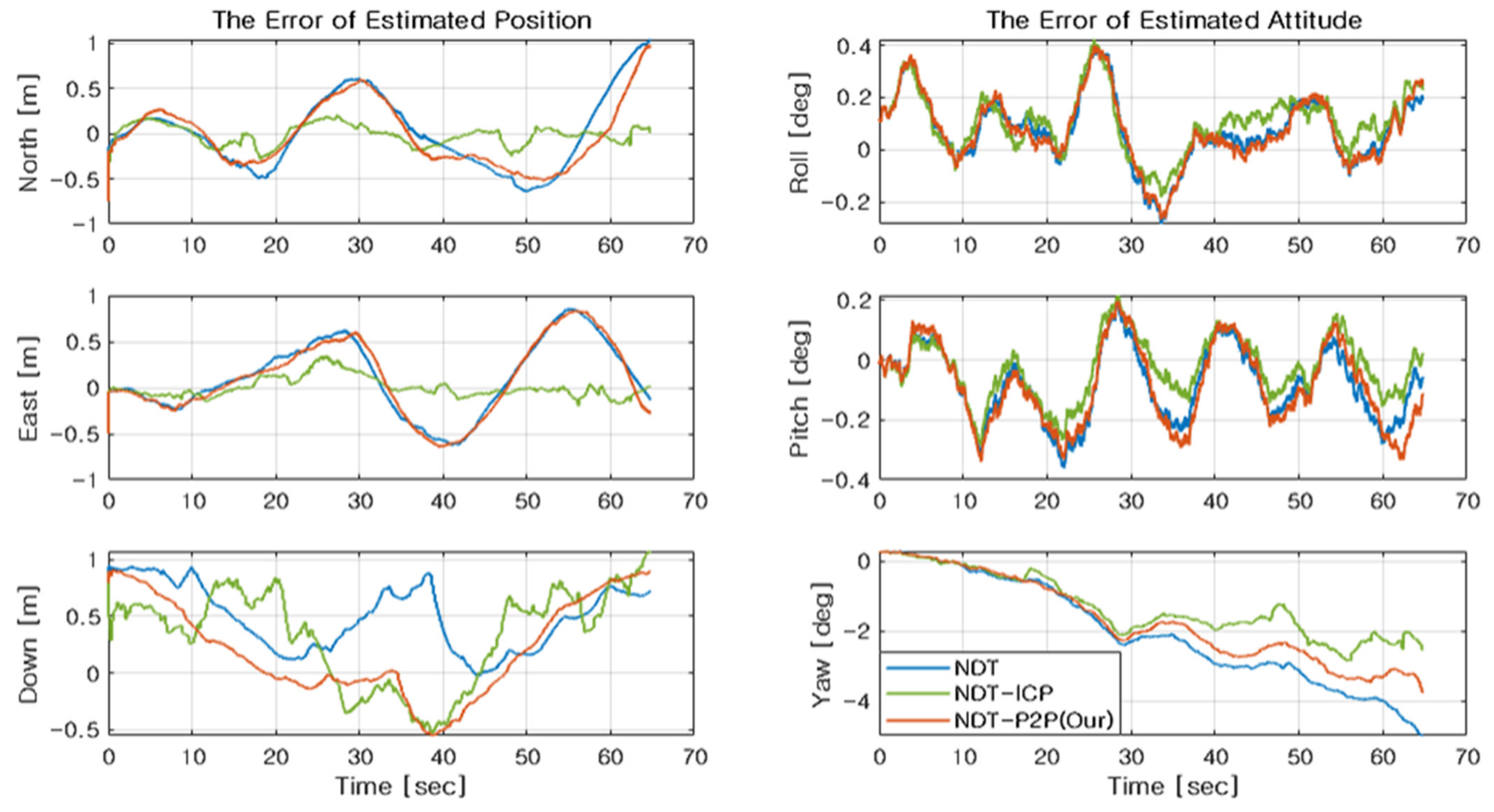
| Position (m) | North | 0.401 | 0.112 | 0.344 |
| East | 0.403 | 0.109 | 0.408 | |
| Down | 0.567 | 0.531 | 0.474 | |
| 2D | 0.569 | 0.157 | 0.534 | |
| 3D | 0.803 | 0.554 | 0.714 | |
| Attitude (°) | Roll | 0.151 | 0.155 | 0.151 |
| Pitch | 0.145 | 0.105 | 0.159 | |
| Yaw | 2.508 | 1.571 | 2.080 | |
| Mapping (Preprocess) | Localization | |
|---|---|---|
| LiDAR | Ouster OS1-16 (3D LiDAR) | Hokuyo UST-20LX (2D LiDAR) |
| Main Board | Intel NUC (i7-8559U) | NVIDIA Jetson Xavier NX |
| IMU | - | ADIS16448 |
Publisher’s Note: MDPI stays neutral with regard to jurisdictional claims in published maps and institutional affiliations. |
© 2021 by the authors. Licensee MDPI, Basel, Switzerland. This article is an open access article distributed under the terms and conditions of the Creative Commons Attribution (CC BY) license (https://creativecommons.org/licenses/by/4.0/).
Share and Cite
Park, G.; Lee, B.; Sung, S. Integrated Pose Estimation Using 2D Lidar and INS Based on Hybrid Scan Matching. Sensors 2021, 21, 5670. https://doi.org/10.3390/s21165670
Park G, Lee B, Sung S. Integrated Pose Estimation Using 2D Lidar and INS Based on Hybrid Scan Matching. Sensors. 2021; 21(16):5670. https://doi.org/10.3390/s21165670
Chicago/Turabian StylePark, Gwangsoo, Byungjin Lee, and Sangkyung Sung. 2021. "Integrated Pose Estimation Using 2D Lidar and INS Based on Hybrid Scan Matching" Sensors 21, no. 16: 5670. https://doi.org/10.3390/s21165670
APA StylePark, G., Lee, B., & Sung, S. (2021). Integrated Pose Estimation Using 2D Lidar and INS Based on Hybrid Scan Matching. Sensors, 21(16), 5670. https://doi.org/10.3390/s21165670