Abstract
IoT technologies enable millions of devices to transmit their sensor data to the external world. The device–object pairing problem arises when a group of Internet of Things is concurrently tracked by cameras and sensors. While cameras view these things as visual “objects”, these things which are equipped with “sensing devices” also continuously report their status. The challenge is that when visualizing these things on videos, their status needs to be placed properly on the screen. This requires correctly pairing visual objects with their sensing devices. There are many real-life examples. Recognizing a vehicle in videos does not imply that we can read its pedometer and fuel meter inside. Recognizing a pet on screen does not mean that we can correctly read its necklace data. In more critical ICU environments, visualizing all patients and showing their physiological signals on screen would greatly relieve nurses’ burdens. The barrier behind this is that the camera may see an object but not be able to see its carried device, not to mention its sensor readings. This paper addresses the device–object pairing problem and presents a multi-camera, multi-IoT device system that enables visualizing a group of people together with their wearable devices’ data and demonstrating the ability to recover the missing bounding box.
1. Introduction
The advance of IoT technologies enables millions of devices to transmit their sensor data to the external world. On the other hand, empowered by deep learning, today’s computer vision has significantly improved its object recognition capability. When an IoT device is placed on an object, we intend to not only recognize the object in videos but also recognize the IoT device bundled with the object.
Surveillance systems are widely used in homes, buildings, and factories. However, when abnormal events occur, it usually takes a lot of human effort to check the surveillance videos. With the advance of AI technologies, automatically analyzing video content becomes feasible. RetinaNet [1] and You Only Look Once (YOLO) [2] can identify a variety of objects with high accuracy and efficiency. OpenPose [3] and Regional Multi-person Pose Estimation (RMPE) [4] can perform human pose recognition without using depth cameras or ToF (time-of-flight) sensors.
In most surveillance and security applications, the central issue is to capture abnormal people, objects, and events in the environment. This work studies the device–object pairing problem in surveillance videos. Previous and common practices include, but are not limited to, barcode, Radio Frequency ID (RFID), and biometric sensing (e.g., fingerprint and iris recognition). However, these methods require keeping at a very short distance to devices. On the other hand, facial recognition relies on obtaining a face database and does not work under larger shooting angles and occlusions. Furthermore, there are privacy concerns in public domains. Another way to identify persons is to exploit IoT devices, such as smartphones and smartwatches, which have become virtually the users’ IDs. Personal devices can also store owners’ profiles and be used in sensitive domains such as factories, hospitals, and restricted areas [5,6]. Further, with the global deployment of 5G, IoT devices nowadays can communicate almost anywhere. When tracking a group of people by camera, it would be nice to also know their purchase histories and preferable social network tools on their smartphone. This motivates us to study combining computer vision and IoT devices under multi-camera environments.
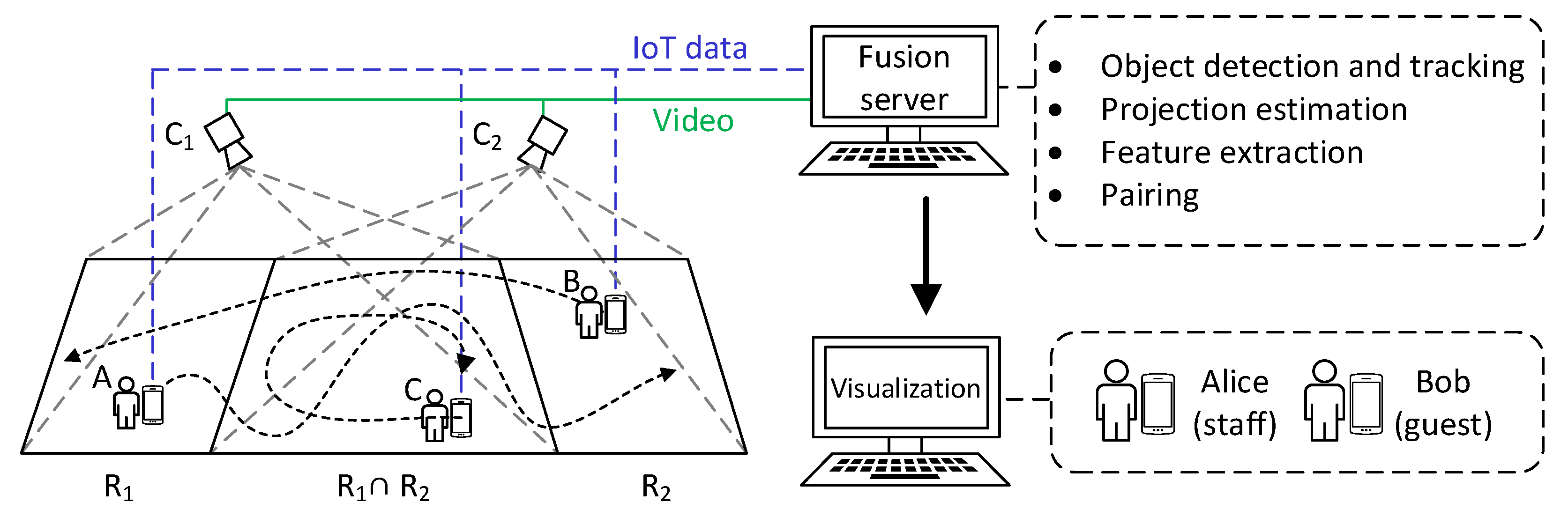
The device–object pairing system considers an environment consisting of multiple cameras, with users wearing their IoT devices walking around. Figure 1 shows our system scenario. There is an IoT network for collecting data from cameras and wearable IoT devices in the environment. We use a YOLO module to obtain and track the human objects appearing in the cameras. The homography matrices of these cameras are estimated to transform each camera view to common surface space. Because there are multiple cameras that concurrently capture the same set of people, the possibilities of occlusions and tracking failures are reduced. Our system then tries to extract objects’ motion features from both visual and wearable sensors and generates (devices, object) pairs that can be displayed on video objects. Therefore, with IoT devices serving as the personal identification of users, our system can visualize user identities and sensor data for smart surveillance.
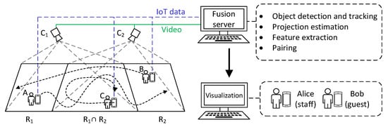
Figure 1.
The device–object pairing system architecture.
We have built a prototype system that runs at 12 Frames Per Second (FPS). It contains a server and two cameras and wearable devices connected by Wi-Fi networks. We designed three mobility patterns (namely random, following, and mimicking) to evaluate its performance.
2. Related Work
Surveillance has been a critical issue in smart city for decades. The study in [7] is an early work that shows how a camera with an embedded system and network connection works for smart analysis. Reference [8] proposes sensor-based surveillance with interactive multiple models to track targets. To solve the person re-identification problem, Reference [9] designs a temporal residual learning module to learn the feature of pedestrian sequences. To monitor illegal or suspicious activities, extracting skeletons by deep learning from video frames is studied in [10]. Our research work is more extensive because we consider both video and sensor data.
Human detection technologies have been rapidly developed recently. Reference [11] proposes detecting objects by a Haar Feature-based Cascade Classifier. With the advance of artificial intelligence, References [1,2] achieve real-time detection by deep learning. Skeletons can be extracted from a mono camera frame in [3,4]. For Multiple Object Tracking (MOT), Reference [12] proposes a k-shortest paths algorithm, Reference [13] adopts a Kalman filter, and [14] uses a deep learning approach. Multi-camera, multi-person tracking by homography matrices is studied in [15]. In the city-scale environment, reference [16] addresses vehicles re-identification and tracking under a multi-camera scenario. Another multi-camera pedestrian tracking is proposed in [17], in which the IoT devices are edge nodes to analyze video by a deep learning module. A sensor-based IoT architecture for smart surveillance is proposed in [18]. A wireless video surveillance system is presented in [19]. On the contrary, our work explores both wearable devices (with sensors) and cameras.
Sensor fusion-based tracking has been studied in a simpler environment. Reference [20] uses a depth camera to extract skeletons and pair them with the Inertial Measurement Unit (IMU) devices carried by users. Fusion-based human and object tracking is shown in [21]. In [22], they use a camera to capture human motion by OpenPose [3] and match the motion with an IMU device to address ID association. These works all exploit user movements to identify persons. Nevertheless, their detection ranges are limited since skeletons can only be detected within a short distance. Reference [23] addresses the fusion of hand gestures and wearable sensors to identify people in crowded mingle scenarios, but it still requires a short distance to track the movements. Reference [24] is an example using a Received Signal Strength Indicator (RSSI) of Wi-Fi as signal trajectories to pair a person on camera. However, the system is unstable since the RSSI signal may suffer more interference and the variance is large. Reference [25] demonstrates how to tag personal ID on people from a drone camera through trajectory pairing. However, it is limited to one drone. Fusing computer vision and the 5G network for driving safety is proposed in [26]. A reconfigurable platform for data fusion is presented in [27].
In this work, we develop machine learning-based feature extraction and a more efficient fusion model with time synchronization under multi-camera environments.
3. Fusion-Based Device–Object Pairing
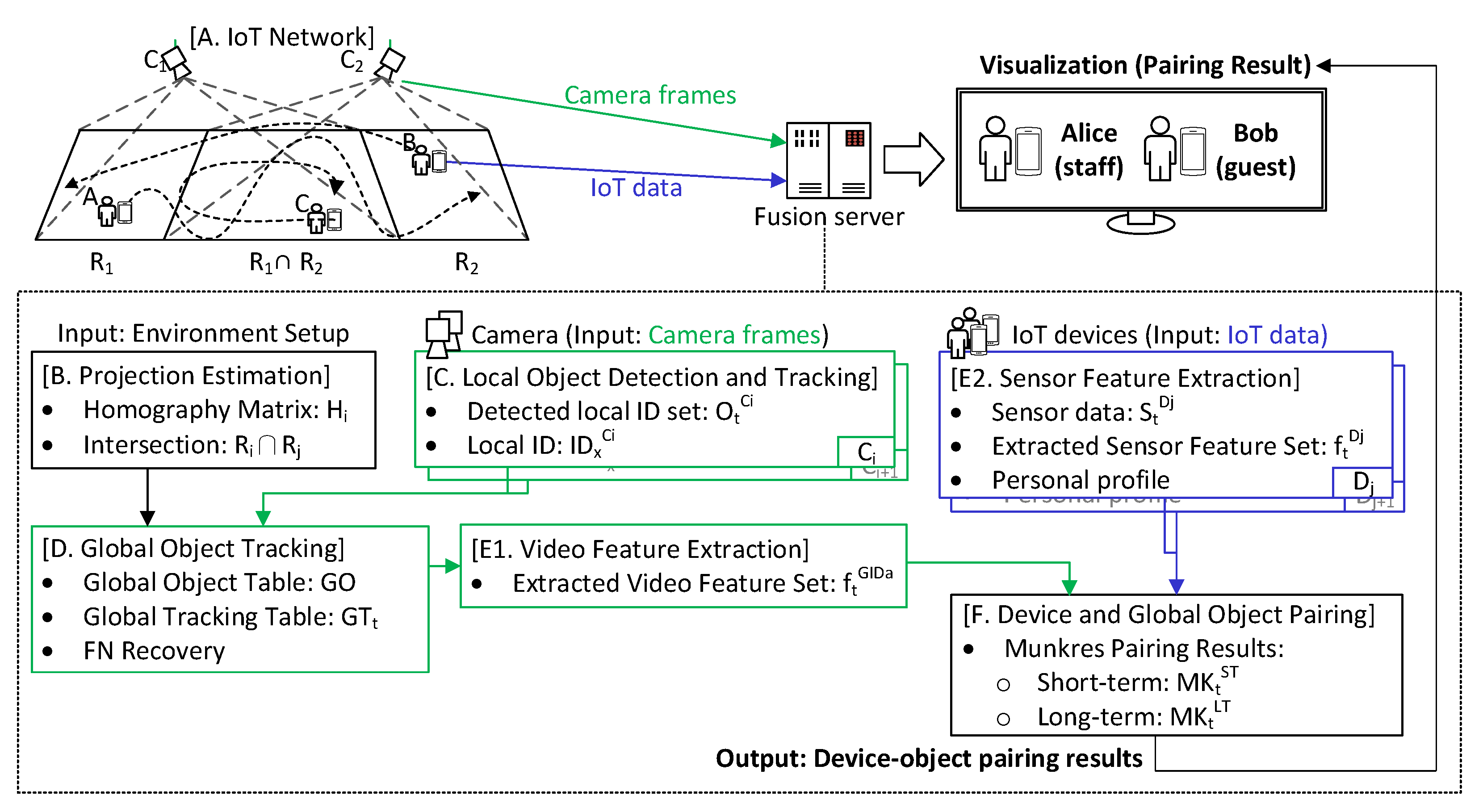
Figure 2 shows the proposed data fusion process. The hardware components include multiple surveillance cameras, some smart wearable devices with built-in IMU (accelerometer and magnetometer), a fusion server, and an IoT network. To pair devices with video objects, the data collected from cameras and wearable devices will be fused based on features extracted. The main software components include: (A) IoT network, (B) projection estimation, (C) local object detection and tracking, (D) global object tracking, (E) feature extraction, and (F) device and global object pairing. Section 3.1 introduces our IoT network. How to map camera views to a common ground space is addressed in Section 3.2. The object tracking task for each camera is discussed in Section 3.3. How to merge all cameras’ views to a global view is addressed in Section 3.4. Then, feature extraction and device–object pairing are covered in Section 3.5 and Section 3.6, respectively.
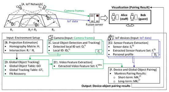
Figure 2.
Data fusion procedure.
3.1. IoT Network
In our system, multiple cameras are deployed to fully cover the surveillance site. Users appearing in front of cameras are expected to put on their wearable devices (otherwise, such users will be marked as “unknown” by the pairing module). An IoT network is designed to manage these devices. Data are exchanged by MQTT (Message Queuing Telemetry Transport [28]), which is a lightweight, publish–subscribe protocol allowing message transportation among massive devices without obvious latency. Furthermore, NTP (Network Time Protocol) is adopted to synchronize time among all components.
For convenience, we use smartphones to simulate wearable devices. Each smartphone has IMUs, including a three-axis accelerometer and magnetometer. These sensors periodically report their data to the fusion server at a rate of 50 Hz in JSON format [29]. Readings are marked by timestamps and pre-processed by a low pass filter. Furthermore, each device is uniquely distinguishable by its ID.
There are multiple cameras. For each camera, an M-JPEG (Motion Joint Photographic Experts Group) server is set up for streaming frames by HTTP (Hypertext Transfer Protocol) in the JPEG format. To validate our framework, we do not use the keyframe method [30], where complete frames are interleaved by compressed frames, causing broken textures when a frame is lost. Therefore, all frames are complete frames, and no retransmission is performed. Every frame from camera is assigned a timestamp t and is denoted as . Frames are remapped to solve the radial distortion problem caused by lens, which is achieved by using the chessboard photos test [31] to calculate the internal and external parameters and the lens distortion coefficients.
3.2. Projection Estimation
To relate the views among multiple cameras, we shall map the pixel space of each camera to a common ground space. Our approach is to estimate a homography matrix for each camera that transforms each camera pixel to a ground coordination. Let the errors caused by the transformation follow a normal distribution model and the coverage region of be . We show how to determine (i) , (ii) and (iii) for each pair of and .
To find , we design a lightweight human-assisted process. We place only a few markers on the ground and send a designated person to walk in the field arbitrarily. The person passes these markers from time to time. Whenever passing a marker, they will stop for a while and record the measured value before moving forward. This stopping behavior serves as an indication to cameras that they are right on a marker. In addition, another wearable device is attached to trace them. In some sense, the cameras localize the person when they stop at a marker, and the wearable sensor tracks their trajectory between two markers while walking. By calibrating their location to a marker, the drifting problem of IMU tracing is significantly relieved. This procedure can be repeated arbitrarily for all camera coverage regions, and during the procedure, the person’s ground trajectory is mapped with camera views to learn the mapping between pixels and ground trajectories. Lots of such mappings can be found only within a few minutes.
In fact, the above steps serve as a labeling process to map ’s pixel space to the ground space. Through object detection, the center of a human object is regarded as their location in ’s pixel space. Their trajectory in is then partitioned into segments (called s) according to those stopping points (markers). On the IMU side, their trajectory is also partitioned into segments (called s) at places where reports stopping events. An is modeled by the recursion: , where is the location of the starting marker, is their location at the k-th stride, is the normalized vector of the k-th stride (obtained from magnetometer), and is a predefined value. The recursion stops when encountering the next marker. We then match the endpoints of all s to ground markers by the maximal likelihood of inter-marker distances and absolute distances. This derives the ground markers of all s’ endpoints. With known endpoints of each , we calibrate it by rescaling. Therefore, we obtain many pairs for each camera with their pixel locations labeled by the .
Given a large number of pairs for , we can derive its homography matrix for the projection. By [32], the objective is to meet
where is a pixel and a ground point. It requires at least four pairs to solve . As an is more likely to contain errors due to sensor data drifting, we suggest retrieving more knowns to minimize the drifting problem. We then apply the least-square method to find .
Assuming the projection error of following a normal distribution, , we collect all calculated by and its corresponding label recorded by IMU. The distances between all and are mapped to a normal distribution to find and of .
By mapping all pixels of to the ground, we can obtain the coverage of . The next task is to find the intersection for each pair of and . The shape of is close to a polygon. Therefore, the overlapping area is also close to a polygon. The related backgrounds can be found in [33,34].
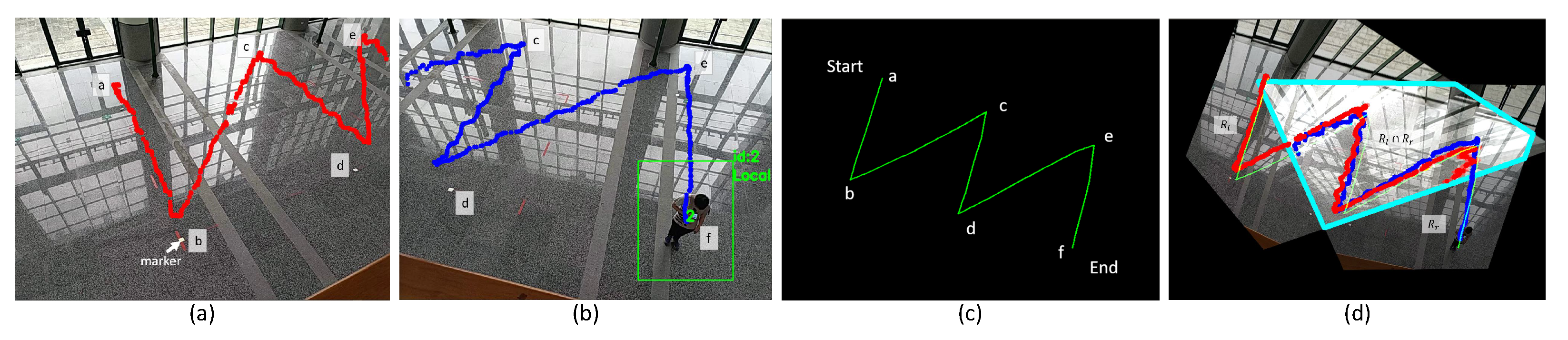
Figure 3 shows an example. Figure 3a,b are views taken by and at the same time. There are six tiny markers on the ground (we do not require cameras to recognize these markers). Through human detection, trajectories of people are obtained. Meanwhile, wearable sensors also derive their trajectories. Figure 3c shows the rescaled IMU trajectories. Finally, by and , the overlapping region is obtained in Figure 3d.
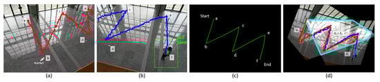
Figure 3.
(a) Trace found by . (b) Trace found by . (c) IMU trajectory partitioned by markers. (d) Overlapping region .
3.3. Local Object Detection and Tracking
Each camera needs to detect and track human objects locally. Since this task has been extensively researched, we will only discuss how we use existing tools to solve this problem. First, for each , it is sent to YOLOv3 [2], a real-time deep learning model for object detection, to retrieve a set of bounding boxes representing detected human objects. We have also tried skeleton models by OpenPose [3], but since the detection time is longer, we adopt YOLO in the rest of the discussion.
Second, we need to determine if a human object detected in has also appeared in . This is achieved by Simple Online and Realtime Tracking (SORT) [13], a tracking algorithm based on the Kalman filter. The outputs are a detected ID set corresponding to all bounding boxes and a miss ID set . We call the local ID assigned to object x at time t by camera . If appears in both and , object x is regarded as the same person. On the other hand, false negative (, but x is not detected as an object at t) and ID switching (x receives different IDs at and t) may happen. If an object in disappears in , the corresponding predicted bounding boxes from Kalman filter are included in . In fact, ID switching is not uncommon when YOLO continuously fails to detect an object or network packets are lost continuously, making SORT regard it as a new person after it reappears. It also happens when a detected bounding box drifts far away from its previous location in a new frame. We will discuss how to reduce such confusion later.
3.4. Global Object Tracking
The next objective is to merge all s detected by all cameras under a global domain. Assume that at time a Global Tracking table as shown in Figure 4 is obtained. The contents of include: (i) the local ID () assigned to object x, (ii) the source camera that captures x, (iii) the global ID () assigned to x, and (iv) the trajectory of x. Note that a may be associated to multiple s if the object is captured by more than one camera.
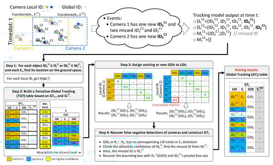
Figure 4.
An example of creating from .
We need to construct at t from . There are four tasks:
- For each object or , and each , find x’s location on the ground space.
- Build a Tentative Global Tracking table ().
- Assign existing or new s to s.
- Recover false negative detections of cameras and construct .
The first task can be achieved by of . Here, we regard the central pixel of an object’s bounding box as its location. The corresponding result is denoted as .
The second task is to build based on and the new tracking results . has the same three entries as (i.e., , , and ). We copy into with three modifications: (i) For each in , we exclude it in since the object is not detected at t. (ii) Depending on the detection confidence at t, for each , only the entry with the highest confidence is kept. (iii) If two s at become very close to each other at t, they will be merged into one (we keep the earlier comer here). For example, in Figure 4, and disappear at t, so they are removed. Furthermore, and become too close, the latecomer is merged with the earlier comer .
The third task is to assign s to s. First, distance matrices between all s and all s of all cameras are built. Given a and a local detected by , we define as the Euclidean distance between the location of and (when and fall in the same row in , the distance is 0). Then we run the Hungarian Matching algorithm [35,36] to pair s and in the distance matrix. Since the matched pairs might encounter a false negative match, we execute a threshold test by checking each matched object (with the highest detection confidence) in and the corresponding paired object . Let . The confidence that and belong to the same global object is written as . Intuitively, is the confidence that an object at an error distance of is acceptable. An example is shown in Figure 4. Note that a pair with distance 0 is always matched (so they can be optimized from the Hungarian algorithm). For a LID that is not matched with a in the above process, or the remainder, a new is assigned to it ( and is such cases). The final results are a number of pairs.
In the fourth task, we first recover false negative detections for each . As we have the intersection region for each pair of and , if there is a discrepancy such that an appears in but no corresponding exists in ’s detection, a miss detection may happen for . We select the best matched missing in , and test its predicted location from SORT against ’s detection . If the test is passed, we can recover the missing bounding box by applying on and the predicted box size from , and add it to ’s local detection list . The new bounding box of should belong to the same of ’s. Finally, we can compile all pairs to construct the at t.
3.5. Feature Extraction
In order to pair video objects with devices, we have to extract some common features to compare their similarity. Let and be the features extracted from the video trajectory of and device , respectively, within a sliding window . We will derive two features, activity type and moving direction. For the activity type of , there are four types, 0 for standing, 1 for walking, 2 for turning-left, and 3 for turning-right. To train a Support Vector Machine (SVM), we feed mean, standard deviation, upper and lower quarter, and median absolute deviation of a number of key sequences as inputs, where a time slot is a basic unit of a sliding window:
- : distance between each sampling point in a time slot.
- : angle between each sampling point in a time slot.
- : axis between each sampling point in a time slot.
The classification result is denoted as . For the activity type of , it is derived by the following key sequences:
- Three-axis accelerometer reading.
- Three-axis magnetometer reading.
In addition, by SVM, the classification result is denoted by .
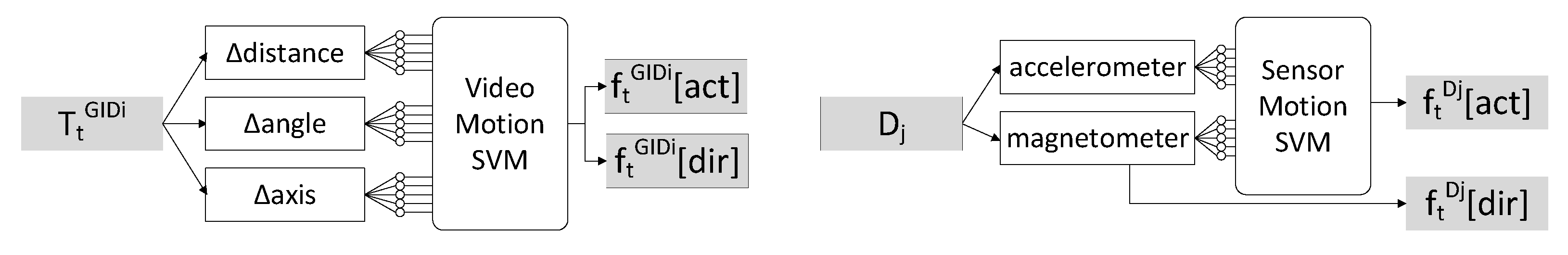
The moving direction is a 2D normalized vector in the world space. The moving direction of is denoted by and is calculated by the starting and ending sampling points in each time slot. The moving direction of is denoted by , which is converted directly from the magnetometer. The value is stabilized by linear regression. Figure 5 illustrates the above procedure for video data and sensor data. ’s trajectory is taken from of , while the input from device is directly taken from its sensors.

Figure 5.
Feature extraction procedure for and .
3.6. Device and Global Object Pairing
By comparing the similarity between and , we try to determine if and are a pair. We will calculate two matrices: (i) short-term distance matrix and (ii) long-term weight matrix . These matrices include all GIDs and devices. By considering short- and long-term relations, we try to obtain more stable pairing results.
The matrix is formed by the distances between all , pairs. Recall vectors , , and . We define short-term distance as
where is the distance between two vectors by normalizing to the range [0, 1]. We then apply Hungarian matching on matrix to find the set of pairs denoted by . Note that this only reveals the result within the sliding window . The long-term weight matrix is formed by considering a sequence of short-term results, namely . For each pair, we define long-term distance as
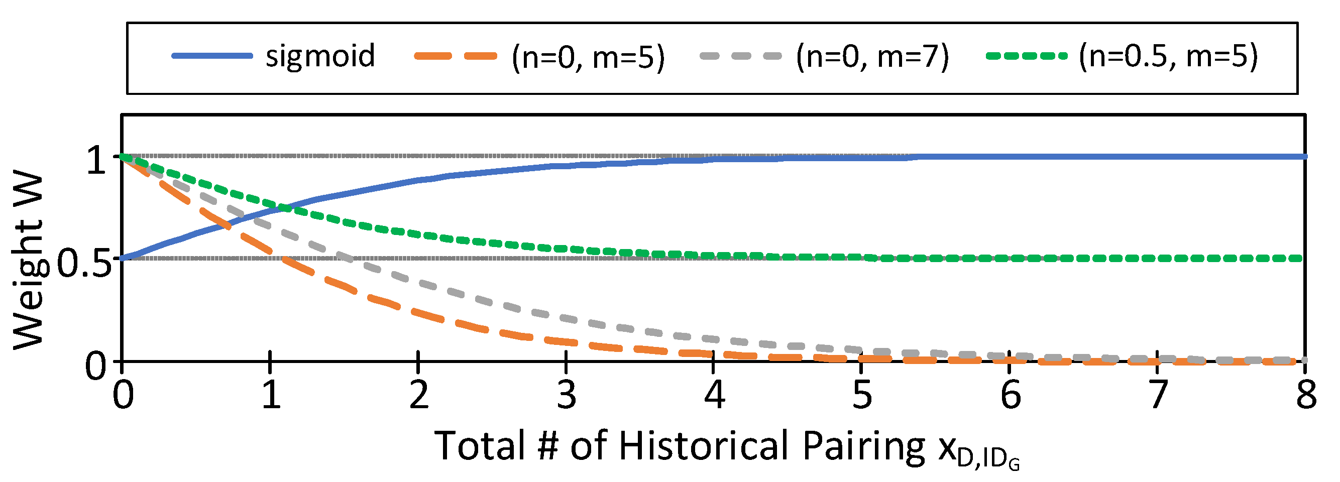
where is the number of times that appears in , , ..., . Equation (2) is to simulate an inverse sigmoid function, where n is the convergence limit, m is the value of to meet n, and 5 is a fine-tuned value. Figure 6 shows under different n and m as opposed to a typical sigmoid function.
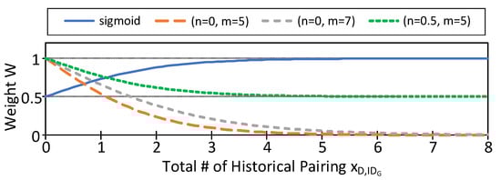
Figure 6.
Equation (2) under different parameters.
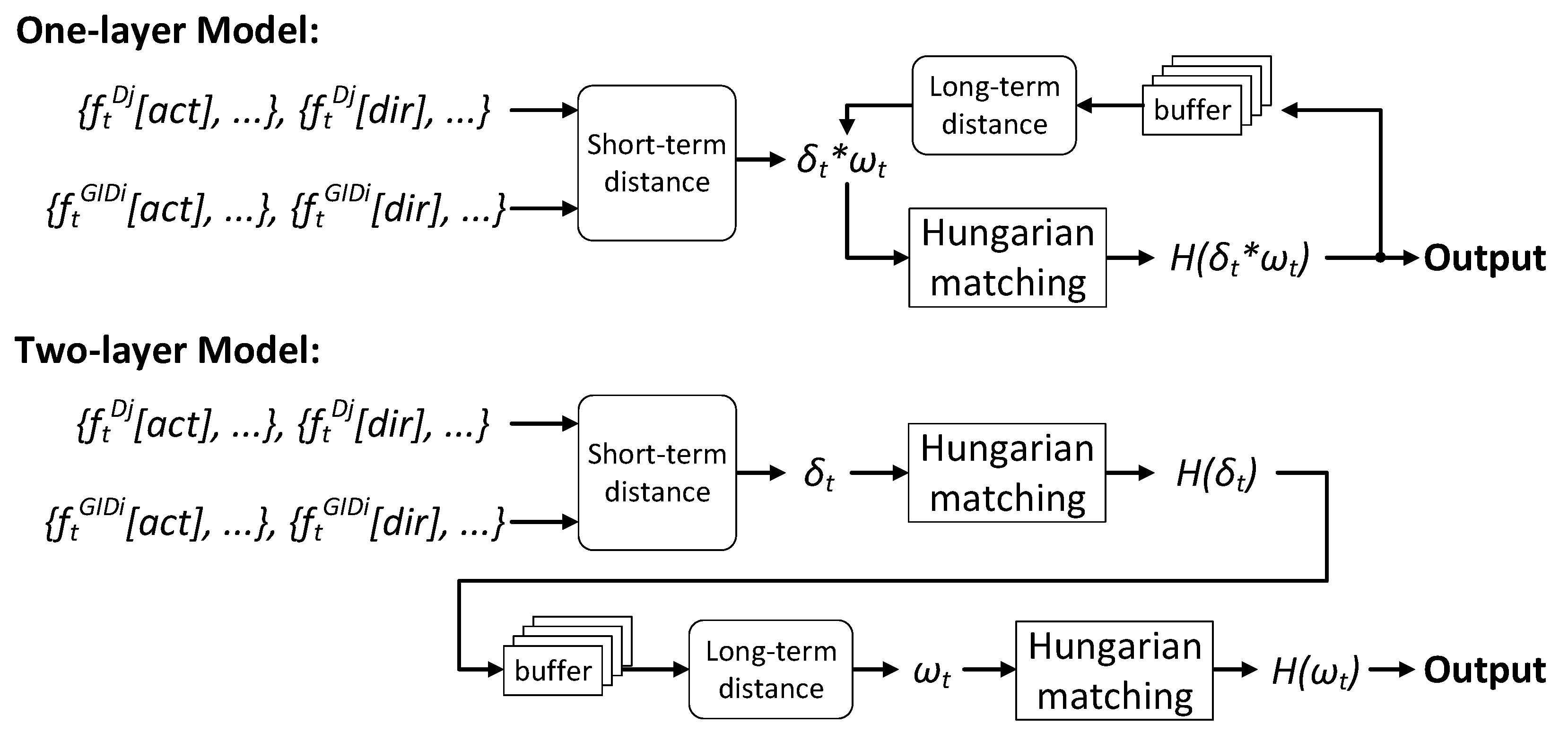
Based on and , we propose two pairing models in Figure 7. The one-layer model uses only one Hungarian matching, which takes accumulated as inputs, where ∗ means pairwise multiplication. However, we find it to be weak in handling the ID exchange problem during tracking. Therefore, we propose the two-layer model by applying Hungarian matching twice, the first time on and the second time on . We will validate this claim by experiments.
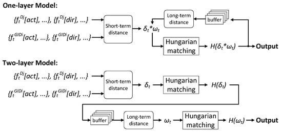
Figure 7.
The proposed one-layer and two-layer pairing models.
4. Performance Evaluation and Discussion
4.1. Experimental Setting
We built a prototype, which consists of two Nokia 8.1 smartphones to simulate IP cameras. We set their height to six meters, view angle to 50 degrees down, and resolution to 600 × 800 pixels. These phones connect to an IEEE 802.11ac access point and stream videos at 20 FPS to our fusion server. Wearable devices are simulated by Android smartphones, which also connect to our fusion server and transmit sensor data at a rate of 50 Hz. The wireless router is ASUS RT-AC86U with a Cortex A53 1.8 GHz dual-core processor and 256 MB RAM. Its claimed rate is 1734 Mbps under 802.11ac and 450 Mbps under 802.11n. Our fusion server has an Intel i7-9750H CPU with six cores, 32 GB RAM, and a RTX 2080 MAX-Q GPU. To speed up the detection speed of YOLOv3-608 (which resizes images to 608 × 608), we added an external RTX 2080 eGPU. Table 1 shows the respective processing time. Processing one frame takes 0.081 s, which approximates to 12 FPS in real-time. This value is calculated from a 5-min clip with processing around 6000 frames. Table 2 shows the activity recognition results of our SVM model, where V-SVM is video motion SVM, and S-SVM is sensor motion SVM. It is trained by a 12-min video by taking 80% data for training and 20% for testing. The accuracies are 97.5% and 99.6% for classifying the four motions from video and sensor data, respectively. The precision and recall are around 95% to 98% for four types of motions. The results show that SVM models are reliable for obtaining motion features.

Table 1.
Processing time of major components.
Table 2.
Evaluation of SVM activity recognition models.
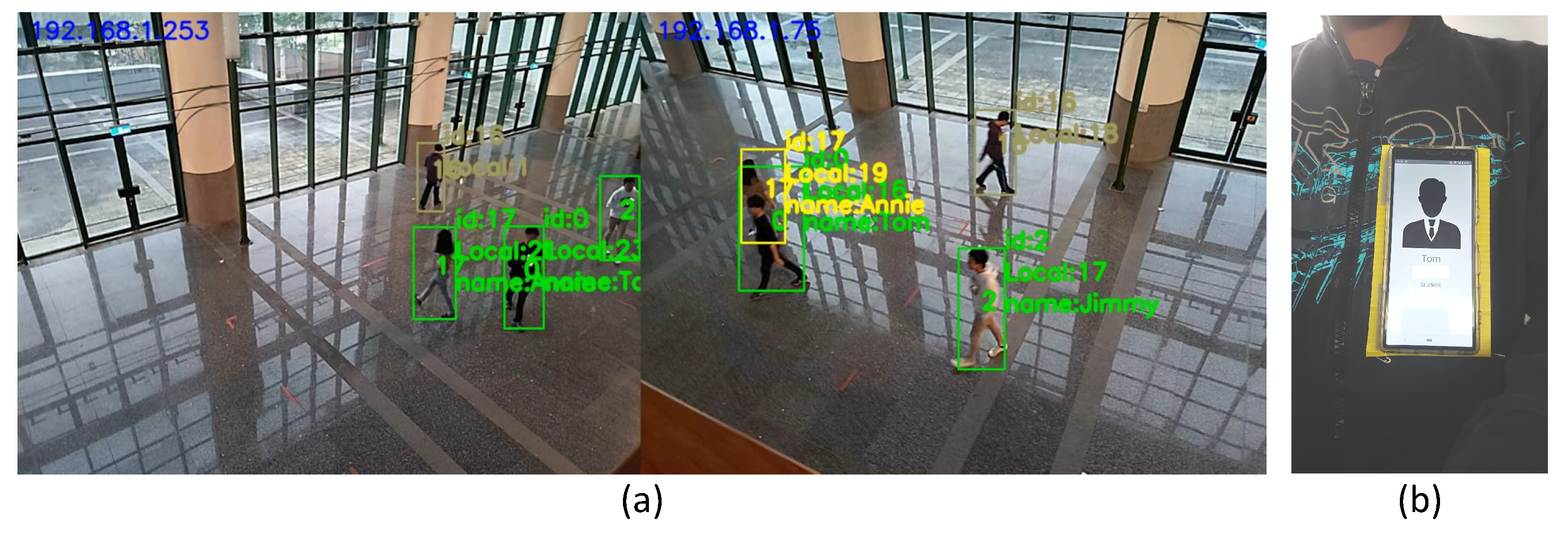
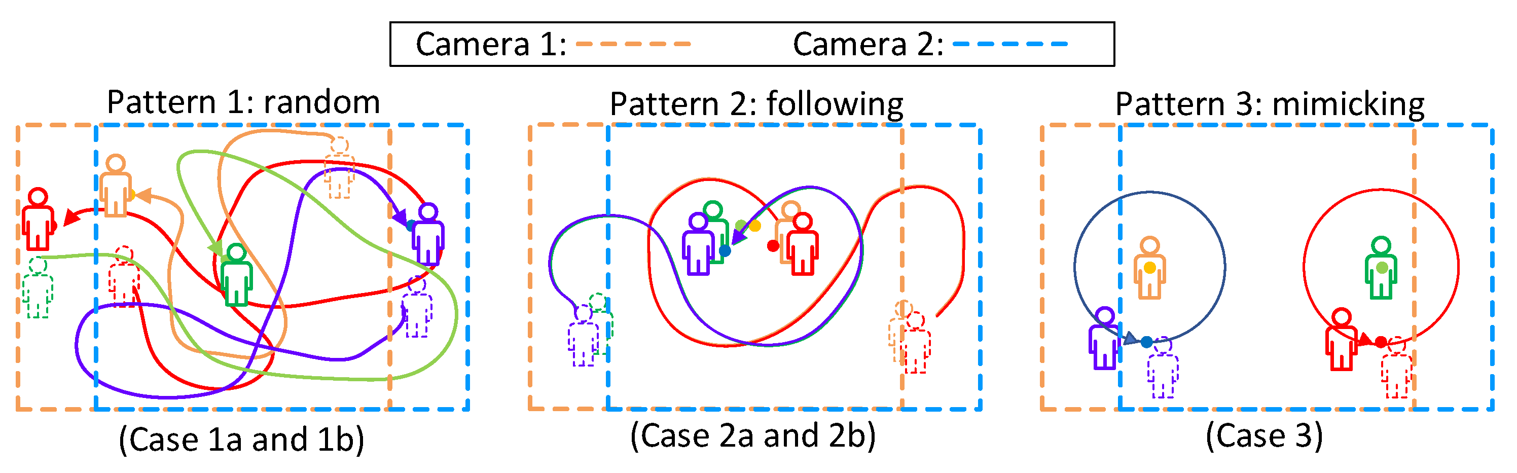
Figure 8 shows our experimental scenario. We invited four testers to walk under the cameras. Three of them wear a smartphone on their chests, as shown in Figure 8b. The last one is a guest without any device. In Figure 8a, an identified person will be tagged as a green bounding box with its corresponding profile. The yellow bounding box indicates the result of recovered missed detection, which will be discussed in Section 4.3. We designed three mobility patterns, as shown in Figure 9. Pattern 1 is a random walk to observe tracking ability when people are walking freely inside the area. We generated two trials. Case 1a and 1b are two different random trajectories. Pattern 2 is following with multiple interleaving, which may cause an ID switch due to SORT [13], because SORT does not consider the target’s visual features on frames. We also generated two trials (2a and 2b) for pattern 2 to observe the ID switch issue. Our system can solve this issue by recovering the lost bounding box. Pattern 3 is trajectory mimicking to simulate that people have similar moving patterns. Since the moving patterns are similar, we generated one trial (case 3) for pattern 3. In each case, video clips and sensor data were collected for 5 min.

Figure 8.
(a) Experiment scene. (b) Smartphone setup on chest.
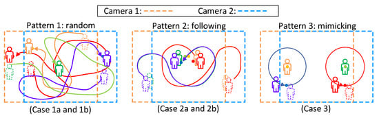
Figure 9.
Mobility patterns for experiments.
Our evaluations are based on four metrics: (i) PITA (Person Identification and Tracking Accuracy), (ii) IDP (Identification Precision), (iii) IDR (Identification Recall) and (iv) IDF1 (Identification F-score 1).
In the above, ObjMiss means missing human object detection (including false positive and negative), and IncPair means incorrect pairing of devices and human objects. TP is the number of true positive pairs, FP is the number of false positive pairs, and FN is the number of false negative pairs.
4.2. Pairing Accuracy
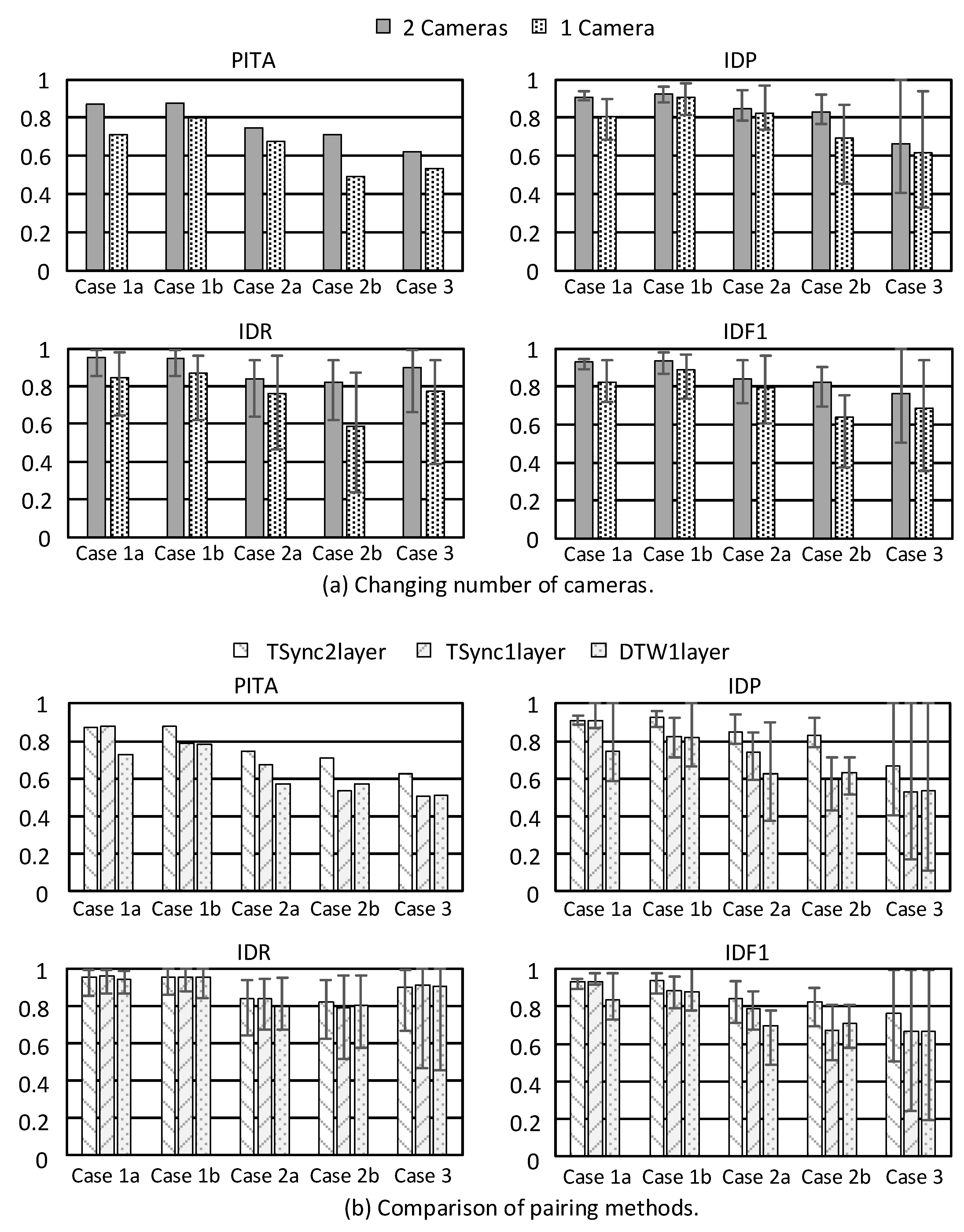
First, we compare single-camera versus multi-camera cases with the two-layer method. Figure 10a shows PITA, IDP, IDR and IDF1 under different mobility patterns. PITA is the accuracy of a whole video clip and sensor data. The value of IDP, IDR and IDF1 is calculated for each person. When more than two people appear in the scene, several pairing results are obtained. We point out the maximum and minimum values in Figure 10 to examine the robustness of our model. Using multiple cameras gives higher accuracy in all cases because it provides more view angles on the environment, thus improving vision recognition capability. On average, accuracy is increased by 10%. The difference between the maximum and minimum value of IDP, IDR, and IDF1 under two cameras is lower than one camera, which means using multiple cameras is more robust.
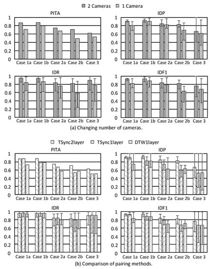
Figure 10.
Pairing accuracy.
Next, we compare the two proposed pairing methods. Here, 1L and 2L mean 1-layer and 2-layer methods, respectively. TSync means using time synchronization; otherwise, Dynamic Time Warping (DTW [37]) will be applied. For Equation (2), n is set to 0.9 for DTW1L and TSync1L, and n is set to 0 for TSync2L. The number m of historical records is set to 10, and the fusion frequency is 2 Hz. Figure 10b shows the results using different pairing methods, where there are always two cameras. We can see that TSync2L performs the best in most cases. For mobility pattern 2, false negative detection occurs due to obstacles. Therefore, TSync1L and DTW1L have much lower accuracy than TSync2L. On average, TSync2L leads by 10% in PITA and IDF1. Considering the difference between the maximum and minimum value, TSync2L is the most robust, and TSync1L outperforms DTW1L.
When DTW is applied, short-term data misalignment may be recoverable. However, it is hard to recover longer misalignment. Therefore, clock synchronization is more important when there are more devices and cameras.
When investigating object tracking, it is common to use an F-score of 1 for comparison. Table 3 shows the detail IDF1 of each person in each case. When the system can not determine the GID of an object, we set it as “unknown”. This would make IDF1 decrease significantly. From Table 3, we can see that IDF1 is greater than 90% under pattern 1. In pattern 2, there are more detection failures, ID switches/exchanges, and occlusions for the computer vision task. Even so, our system can still track people with IDF1 of 80%. Unfortunately, pattern 3 is a challenge to our system because people have similar movements. Our current movement features are unable to distinguish such cases. A possible solution is to explore more detailed features, such as skeleton data, which can be a direction of future work.
Table 3.
Comparison of Per-person IDF1.
4.3. False Negative Recovery Capability
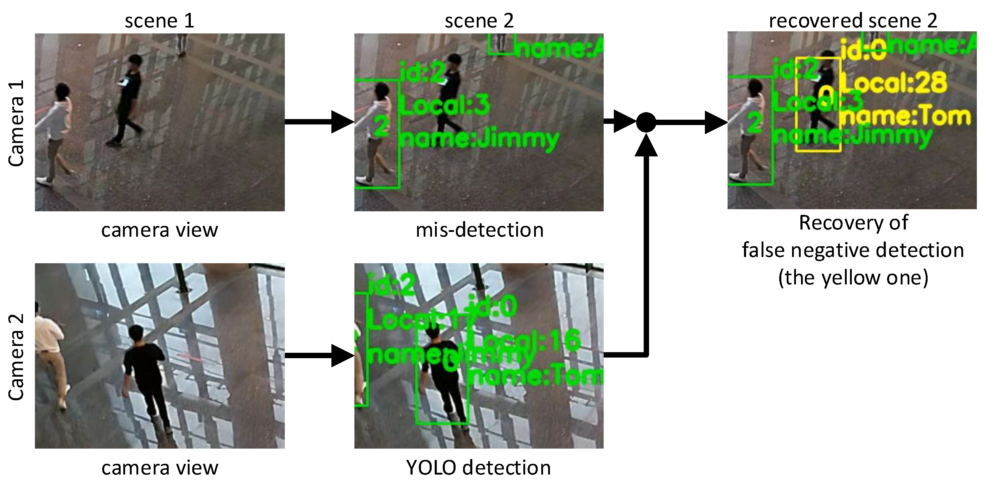
False negative detection is inevitable in image object detection. As shown earlier, this may be recovered by our system in camera intersection regions. In order to observe the recovery capability, we collected 1886 pieces of data in the overlapping area when a person moves in. Ideally, both cameras and should be able to detect and track them. We treat the tracking results of as ground truth. When solving the device–object pairing problem, we assume that cannot detect the person, and then we use the information from to recover the missed detection of . The recovered detection is regarded as a new bounding box of , and then we compare these new bounding boxes against those detected by the same through YOLO. Figure 11 shows a scenario. A person in black clothes is in the overlapping area . Although both and may detect the person, we purposefully remove ’s detection. During the data fusion procedure, we use the information from to recover the lost bounding box on . Then the predicted results for are compared against the ground truth (i.e., the one detected by YOLO). The outcomes are measured by Intersection over Union (IoU), , of these two bounding boxes. An IoU value closer to 1 indicates a better recovery effect.
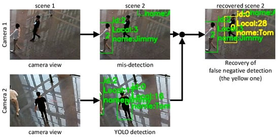
Figure 11.
False negative recovery scenario.
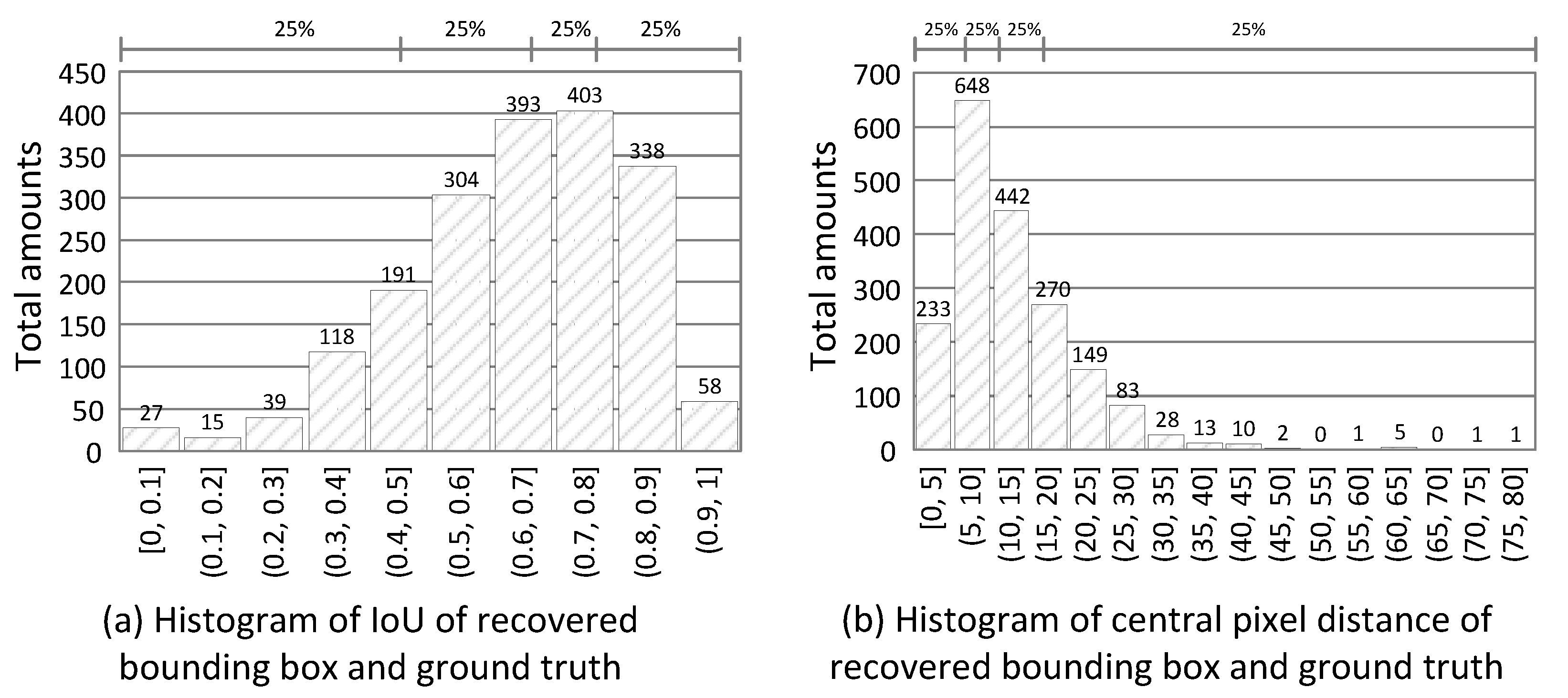
Figure 12a shows the histogram of IoU of these 1886 tests. We see that the top three IoU ranges fall in the (0.6, 0.9] interval, and 50% of results are in the (0.6, 1] interval. Figure 12b shows the histogram of the central pixel distance of two bounding boxes. We see that over 75% of the distances fall in the (0, 15] interval. Even though the view angles of and are different, most of our predicted bounding boxes by can achieve an IoU above 0.7 and a pixel distance of less than 20. On average, the mean IoU is 0.64, and the mean distance is 12 pixels. For surveillance applications, such driftings are acceptable, and thus the solving device–object pairing problem helps us to identify and track people or things from different angles and visualize their sensor data easily.
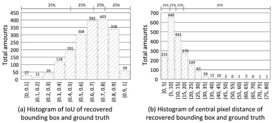
Figure 12.
Evaluation results for false negative recovery.
5. Conclusions
The device–object pairing problem arises as an essential issue in the IoT world when we concurrently track a group of things with both cameras and sensors. Correctly pairing visual objects with their sensor data may enable lots of new applications. For example, in high-value livestock farming, the visual objects can be defined as animals. In an automatic warehouse, we can treat the robots as visual objects. Based on our system, we can interpret the status of visual objects with sensor information. This work proposes a device–object pairing system consisting of multiple cameras and wearable devices. The overlapping area between cameras can be used for detecting identical objects. When a missed detection occurs, we can use the information from another camera to recover the missing bounding box. We design a lightweight human-assisted process to estimate a homography matrix for each camera that transforms each camera pixel to a ground coordination. The procedure can be finished within a few minutes. To find the relationship between wearable devices and visual objects, we extract motion features from them and then design one-layer and two-layer algorithms to predict possible pairing. A prototype has been built to test the feasibility of our system under several actual scenarios. It also demonstrates the ability to recover the missing bounding box. Future work may be directed to considering larger scales, which involve a more efficient deployment procedure and an IoT platform for device management. In order to improve device–object pairing results, more features, such as sub-meter indoor localization or skeleton recognition, can be taken into consideration.
Author Contributions
Conceptualization, K.-L.T., K.-R.W. and Y.-C.T.; methodology, K.-L.T.; software, K.-L.T.; validation, K.-L.T., K.-R.W. and Y.-C.T.; formal analysis, K.-L.T.; investigation, K.-L.T., K.-R.W. and Y.-C.T.; resources, K.-R.W., Y.-C.T.; data curation, K.-L.T., K.-R.W.; writing—original draft preparation, K.-L.T., K.-R.W. and Y.-C.T.; writing—review and editing, K.-L.T., K.-R.W. and Y.-C.T.; visualization, K.-L.T., K.-R.W.; supervision, Y.-C.T.; project administration, K.-R.W., Y.-C.T.; funding acquisition, Y.-C.T. All authors have read and agreed to the published version of the manuscript.
Funding
This research was supported by ITRI, Pervasive Artificial Intelligence Research (PAIR) Labs, and Ministry of Science and Technology (MoST) under Grant 110-2221-E-A49-033-MY3 and 110-2634-F-009-019. This work is also financially supported by “Center for Open Intelligent Connectivity” of “Higher Education Sprout Project” of NYCU and MOE, Taiwan.
Informed Consent Statement
Informed consent was obtained from all subjects involved in the study.
Data Availability Statement
Not applicable.
Conflicts of Interest
The authors declare no conflict of interest.
Abbreviations
The following abbreviations are used in this manuscript:
| YOLO | You Only Look Once |
| RMPE | Regional Multi-person Pose Estimation |
| FPS | Frames Per Second |
| MOT | Multiple Object Tracking |
| RSSI | Received Signal Strength Indicator |
| IMU | Inertial Measurement Unit |
| JSON | JavaScript Object Notation |
| SORT | Simple Online and Realtime Tracking |
| GT | Global Tracking table |
| LID | Local ID |
| GID | Global ID |
| TGT | Tentative Global Tracking table |
| SVM | Support Vector Machine |
| V-SVM | video motion SVM |
| S-SVM | sensor motion SVM |
| PITA | Person Identification and Tracking Accuracy |
| IDP | Identification Precision |
| IDR | Identification Recall |
| IDF1 | Identification F-score 1 |
| TSync | Time Synchronization |
| DTW | Dynamic Time Warping |
| IoU | Intersection over Union |
References
- Lin, T.Y.; Goyal, P.; Girshick, R.; He, K.; Dollár, P. Focal Loss for Dense Object Detection. IEEE Trans. Pattern Anal. Mach. Intell. 2020, 42, 318–327. [Google Scholar] [CrossRef] [PubMed] [Green Version]
- Redmon, J.; Farhadi, A. YOLOv3: An Incremental Improvement. arXiv 2018, arXiv:1804.02767. [Google Scholar]
- Cao, Z.; Hidalgo, G.; Simon, T.; Wei, S.E.; Sheikh, Y. OpenPose: Realtime Multi-Person 2D Pose Estimation using Part Affinity Fields. IEEE Trans. Pattern Anal. Mach. Intell. 2017, 43, 172–186. [Google Scholar] [CrossRef] [Green Version]
- Fang, H.; Xie, S.; Tai, Y.; Lu, C. RMPE: Regional Multi-person Pose Estimation. In Proceedings of the IEEE International Conference on Computer Vision (ICCV), Venice, Italy, 22–29 October 2017; pp. 2353–2362. [Google Scholar]
- Ceccato, V. Eyes and Apps on the Streets: From Surveillance to Sousveillance Using Smartphones. Crim. Justice Rev. 2019, 44, 25–41. [Google Scholar] [CrossRef] [Green Version]
- Kostikis, N.; Hristu-Varsakelis, D.; Arnaoutoglou, M.; Kotsavasiloglou, C.; Baloyiannis, S. Towards remote evaluation of movement disorders via smartphones. In Proceedings of the International Conference of the IEEE Engineering in Medicine and Biology Society, Boston, MA, USA, 30 August–3 September 2011; pp. 5240–5243. [Google Scholar]
- Bramberger, M.; Doblander, A.; Maier, A.; Rinner, B.; Schwabach, H. Distributed Embedded Smart Cameras for Surveillance Applications. IEEE Comput. 2006, 39, 68–75. [Google Scholar] [CrossRef]
- Vasuhi, S.; Vaidehi, V. Target Tracking using Interactive Multiple Model for Wireless Sensor Network. Inf. Fusion 2016, 27, 41–53. [Google Scholar] [CrossRef]
- Dai, J.; Zhang, P.; Wang, D.; Lu, H.; Wang, H. Video Person Re-Identification by Temporal Residual Learning. IEEE Trans. Image Process. 2019, 28, 1366–1377. [Google Scholar] [CrossRef] [Green Version]
- Rathod, V.; Katragadda, R.; Ghanekar, S.; Raj, S.; Kollipara, P.; Rani, I.A.; Vadivel, A. Smart Surveillance and Real-Time Human Action Recognition Using OpenPose. In ICDSMLA 2019; Springer: Singapore, 2019; pp. 504–509. [Google Scholar]
- Lienhart, R.; Maydt, J. An Extended Set of Haar-like Features for Rapid Object Detection. Proc. Int. Conf. Image Process. 2002, 1, 900–903. [Google Scholar]
- Berclaz, J.; Fleuret, F.; Turetken, E.; Fua, P. Multiple Object Tracking Using K-Shortest Paths Optimization. IEEE Trans. Pattern Anal. Mach. Intell. 2011, 33, 1806–1819. [Google Scholar] [CrossRef] [PubMed] [Green Version]
- Bewley, A.; Ge, Z.; Ott, L.; Ramos, F.; Upcroft, B. Simple Online and Realtime Tracking. In Proceedings of the IEEE International Conference on Image Processing (ICIP), Phoenix, AZ, USA, 25–28 September 2016; pp. 3464–3468. [Google Scholar]
- YuEmail, F.; Li, W.; Li, Q.; Liu, Y.; Yan, X.S.J. POI: Multiple Object Tracking with High Performance Detection and Appearance Feature. In European Conference on Computer Vision; Springer: Cham, Switzerland, 2016; pp. 36–42. [Google Scholar]
- Eshel, R.; Moses, Y. Homography based Multiple Camera Detection and Tracking of People in a Dense Crowd. In Proceedings of the IEEE Conference on Computer Vision and Pattern Recognition (CVPR), Anchorage, AK, USA, 23–28 June 2008. [Google Scholar]
- Spanhel, J.; Bartl, V.; Juranek, R.; Herout, A. Vehicle Re-Identifiation and Multi-Camera Tracking in Challenging City-Scale Environment. In Proceedings of the IEEE/CVF Conference on Computer Vision and Pattern Recognition (CVPR) Workshops, Long Beach, CA, USA, 16–20 June 2019. [Google Scholar]
- Neff, C.; Mendieta, M.; Mohan, S.; Baharani, M.; Rogers, S.; Tabkhi, H. REVAMP2T: Real-Time Edge Video Analytics for Multicamera Privacy-Aware Pedestrian Tracking. IEEE Internet Things J. 2020, 7, 2591–2602. [Google Scholar] [CrossRef] [Green Version]
- Kokkonis, G.; Psannis, K.E.; Roumeliotis, M.; Schonfeld, D. Real-time Wireless Multisensory Smart Surveillance with 3D-HEVC Streams for Internet-of-Things (IoT). J. Supercomput. Vol. 2017, 73, 1044–1062. [Google Scholar] [CrossRef]
- Zhang, T.; Chowdhery, A.; Bahl, P.; Jamieson, K.; Banerjee, S. The Design and Implementation of a Wireless Video Surveillance System. In Proceedings of the ACM International Conference on Mobile Computing and Networking (MobiCom), Paris, France, 7–11 September 2015; pp. 426–438. [Google Scholar]
- Tsai, R.Y.C.; Ke, H.T.Y.; Lin, K.C.J.; Tseng, Y.C. Enabling Identity-Aware Tracking via Fusion of Visual and Inertial Features. In Proceedings of the IEEE International Conference on Robotics and Automation (ICRA), Montreal, QC, Canada, 20–24 May 2019. [Google Scholar]
- Kao, H.W.; Ke, T.Y.; Lin, K.C.J.; Tseng, Y.C. Who Takes What: Using RGB-D Camera and Inertial Sensor for Unmanned Monitor. In Proceedings of the IEEE International Conference on Robotics and Automation (ICRA), Montreal, QC, Canada, 20–24 May 2019. [Google Scholar]
- Ruiz, C.; Pan, S.; Bannis, A.; Chang, M.P.; Noh, H.Y.; Zhang, P. IDIoT: Towards Ubiquitous Identification of IoT Devices through Visual and Inertial Orientation Matching During Human Activity. In Proceedings of the IEEE/ACM International Conference on Internet-of-Things Design and Implementation (IoTDI), Sydney, NSW, Australia, 21–24 April 2020; pp. 40–52. [Google Scholar]
- Cabrera-Quiros, L.; Tax, D.M.J.; Hung, H. Gestures In-The-Wild: Detecting Conversational Hand Gestures in Crowded Scenes Using a Multimodal Fusion of Bags of Video Trajectories and Body Worn Acceleration. IEEE Trans. Multimed. 2020, 22, 138–147. [Google Scholar] [CrossRef]
- Nguyen, L.T.; Kim, Y.S.; Tague, P.; Zhang, J. IdentityLink: User-Device Linking through Visual and RF-Signal Cues. In Proceedings of the ACM International Joint Conference on Pervasive and Ubiquitous Computing, Seattle, WA, USA, 13–17 September 2014; pp. 529–539. [Google Scholar]
- Van, L.D.; Zhang, L.Y.; Chang, C.H.; Tong, K.L.; Wu, K.R.; Tseng, Y.C. Things in the air: Tagging wearable IoT information on drone videos. Discov. Internet Things 2021, 1, 6. [Google Scholar] [CrossRef]
- Tseng, Y.Y.; Hsu, P.M.; Chen, J.J.; Tseng, Y.C. Computer Vision-Assisted Instant Alerts in 5G. In Proceedings of the 2020 29th International Conference on Computer Communications and Networks (ICCCN), Honolulu, HI, USA, 3–6 August 2020; pp. 1–9. [Google Scholar]
- Zhang, L.Y.; Lin, H.C.; Wu, K.R.; Lin, Y.B.; Tseng, Y.C. FusionTalk: An IoT-Based Reconfigurable Object Identification System. IEEE Internet Things J. 2021, 8, 7333–7345. [Google Scholar] [CrossRef]
- MQTT Version 5.0. Available online: http://docs.oasis-open.org/mqtt/mqtt/v5.0/mqtt-v5.0.html (accessed on 3 August 2021).
- Standard ECMA-404 The JSON Data Interchange Syntax. Available online: https://www.ecma-international.org/publications-and-standards/standards/ecma-404/ (accessed on 3 August 2021).
- Romero, A. Keyframes, InterFrame and Video Compression. Available online: https://blog.video.ibm.com/streaming-video-tips/keyframes-interframe-video-compression/ (accessed on 3 August 2021).
- Camera Calibration with OpenCV. Available online: https://docs.opencv.org/2.4/doc/tutorials/calib3d/camera_calibration/camera_calibration.html (accessed on 3 August 2021).
- Basic Concepts of the Homography Explained with Code. Available online: https://docs.opencv.org/master/d9/dab/tutorial_homography.html (accessed on 3 August 2021).
- The Shapely User Manual. Available online: https://shapely.readthedocs.io/en/latest/manual.html (accessed on 3 August 2021).
- Clementini, E.; Felice, P.D.; van Ooster, P. A Small Set of Formal Topological Relationships Suitable for End-User Interaction. In International Symposium on Spatial Databases; Springer: Berlin/Heidelberg, Germany, 1993; pp. 277–295. [Google Scholar]
- Moore, K.; Landman, N.; Khim, J. Hungarian Maximum Matching Algorithm. Available online: https://brilliant.org/wiki/hungarian-matching/ (accessed on 3 August 2021).
- Kuhn, H.W. The Hungarian Method for the Assignment Problem. Nav. Res. Logist. Q. 1955, 10, 83–97. [Google Scholar] [CrossRef] [Green Version]
- Berndt, D.J.; Clifford, J. Using Dynamic Time Warping to Find Patterns in Time Series. In Proceedings of the KDD Workshop, Seattle, WA, USA, 31 July–1 August 1994; pp. 359–370. [Google Scholar]

Publisher’s Note: MDPI stays neutral with regard to jurisdictional claims in published maps and institutional affiliations. |
© 2021 by the authors. Licensee MDPI, Basel, Switzerland. This article is an open access article distributed under the terms and conditions of the Creative Commons Attribution (CC BY) license (https://creativecommons.org/licenses/by/4.0/).