Abstract
Current process of calibrating radiation thermometers, including thermal imagers, relies on measurement comparison with the temperature of a black body at a set distance. Over time, errors have been detected in calibrations of some radiation thermometers, which were correlated with moisture levels. In this study, effects of atmospheric air on thermal transmission were evaluated by the means of simulations using best available resources of the corresponding datasets. Sources of spectral transmissivity of air were listed, and transmissivity data was obtained from the HITRAN molecular absorption database. Transmissivity data of molecular species was compiled for usual atmospheric composition, including naturally occurring isotopologs. Final influence of spectral transmissivity was evaluated for spectral sensitivities of radiation thermometers in use, and total transmissivity and expected errors were presented for variable humidity and measured temperature. Results reveal that spectral range of measurements greatly influences susceptibility of instruments to atmospheric interference. In particular, great influence on measurements is evident for the high-temperature radiation pyrometer in the spectral range of 2–2.7 µm, which is in use in our laboratory as a traceable reference for high-temperature calibrations. Regarding the calibration process, a requirement arose for matching the humidity parameters during the temperature reference transfer to the lower tiers in the chain of traceability. Narrowing of the permitted range of humidity during the calibration, monitoring, and listing of atmospheric parameters in calibration certificates is necessary, for at least this thermometer and possibly for other thermometers as well.
1. Introduction
Nonideal transmissivity of air is known in the field of radiation thermometry; however, the influence of this effect has not been evaluated and is usually neglected in the field. While the effect can be negligible for many radiation thermometer applications, evaluating this effect is of particular importance for improvement of practices in the fields where measurement uncertainty is important, including calibrations of reference thermometers, especially when ensuring traceability to the national standards.
The goal of this study is to analyze available resources of spectral data and calculate spectral transmissivity of air mixture for variable relative humidity, temperature, air pressure, and path length within expected usual atmospheric deviations. Ideally, a simple and fast MATLAB model of spectral transmissivity is to be made for evaluation of effect of thermal radiation transmission in the spectral range of 1 µm–18 µm, indicating the susceptibility of used laboratory equipment to atmospheric interference, and allowing repeated simulations for evaluation of measurement uncertainty in radiation thermometry.
1.1. Significance of the Research
In the Laboratory for Metrology and Quality of the Faculty of Electrical Engineering, University of Ljubljana, calibrations of radiation thermometers have been conducted for more than 20 years. The calibration procedure consists of a reference black body cavity at stabilized temperature, measured by the ITS-90 calibrated reference thermometer. The device in calibration is directed to the black body source from a set distance. Besides the contact thermometers, reference radiation thermometers are often used to measure the radiant temperature as well.
Between the consecutive calibrations of the reference radiation thermometer, drift has been detected, with the magnitude exceeding the total calibration uncertainty. Upon further investigation into causality, the drift has been found to correlate with different humidity levels during the calibration.
Usual calibration procedures of the calibration laboratory assume either total transmission of thermal radiation at short distances or fixed setting with negligible deviations. Regardless, humidity correction is always omitted, whereas the allowed parameter ranges, which are listed in the calibration certificate, are relatively wide. Atmospheric influences should be accounted for in the calibration process, either by matching calibration and target usage parameters, applying correction, and/or expanding calibration uncertainty.
1.2. Existing Works and Research
Earlier attempts of calculating thermal transmission were conducted by Elder and Strong [1] in 1953, where the total transmission was considered as the effect of continuous attenuation of particles and band absorption, also citing Beer’s law. Average influence of particles of water and the effect of pressure were later approximated for eight spectral ranges, from 0.7 µm to 14 µm. Calculation of overall transmission was subsequently reduced to eight estimations of the average radiance and transmissivity and thus limited resolution for calculations of transmission of thermal radiation, especially in the case of uneven spectral emissivity distribution of the radiation source.
Wyat et al. [2] calculated the spectral transmissivity of water vapor and carbon dioxide as a function of wavenumber, pressure, and path-times-length product, computed from vibrational and rotational constants. Included in the computed spectrum were the most strong vibrational transition lines, yielding sufficient resolution, however results were of limited accuracy when compared to measurements by Burch et al. [3].
An experimental concept has recently been proposed by Zhang et al. [4], where total transmissivity of a radiator–imager system is proposed to be calibrated against varying moisture levels in order to measure relative humidity of air with high response rate.
The first detailed computer models for public use were developed by the Air Force Geophysics Laboratory (AFGL). The Fortran-based Low-Resolution Transmission Model (LOWTRAN) [5] was developed with relatively low spectral resolution of 20 cm−1, with intention to simulate effects of the Earth’s atmosphere on transmission of radiation by the Sun, Earth, Moon, and horizontal observers in the lower atmosphere. The Moderate-Resolution Transmission Model (MODTRAN) [6] is the updated model of LOWTRAN, with the improved resolution of 2 cm−1. MODTRAN calculations were based on Voigt line shape, incorporating both the pressure-dependent Lorentz line shape and the temperature-dependent Doppler line shape, improving accuracy of modelling high-altitude atmospheric conditions. Continuation of these models also include Fast Atmospheric Signature Code (FASCODE), Line-By-Line Radiative Transfer Model (LBLRTM) and Combined Atmospheric Radiative Transfer Model (CART) [7]. Updates were focused on improving reliability and precision of molecular absorption parameters and other atmospheric effects, such as incorporating single and multiple scattering, vertical profiles of atmospheric composition, pressure and temperature, and effects of clouds, rain, and airborne particles, with the main focus in the meteorological and climatological fields.
Parallel to the model development, databases of molecular absorption data were compiled, allowing simulation and detection of variable atmospheric composition, pressure, and temperature in far greater ranges then measured in the Earth’s atmosphere. The high-resolution transmission molecular absorption database (HITRAN) [8] is a compilation of theoretically- and experimentally-derived spectral line absorption data by numerous authors, first introduced in 1973 and frequently updated since. This database was well accepted in the scientific community and considered the best source to date.
Accompanying the HITRAN database since the 2012 edition were collision-induced absorption (CIA) spectrums of the most significant binary complexes of molecules in bound, quasi-bound, and free scattered states [9]. The absorption by complexes of more than two molecules was expected to be insignificant and omitted in the database. Hartmann [10] used HITRAN line-by-line data, as well as FORTRAN simulated collision induced absorption data to isolate N2 absorption spectrum near 2.16 μm and to measure nitrogen content of the Earth’s atmosphere. Validation of CIA simulation was performed by fitting absorption spectrum to the difference in balloon-borne and ground-based (solar zenith angle ≥ 87°) measurements of solar radiation. Fitting residuals were shown to improve from 5% without collision-induced absorption to 2% with collision-induced absorption, whereas the measurement-fitted N2 content parameter 0.783 ± 0.022 successfully corresponded with the expected reference value of 0.7809. Hartmann’s N2 Air CIA spectrums were also included in the most recent (2016) edition of the HITRAN CIA database.
2. Materials and Methods
2.1. Calculation of Moist Air–Gas Ratios
According to Dalton’s law, partial pressure of sum of all dry gases is reduced proportionately when an amount of water vapour is added at a constant atmospheric pressure . Assuming a constant molar composition of dry air, partial pressures of individual gases are equally reduced when water vapor is added, which should not be true for real gas components with different individual compressibility factors.
Ideality of Dalton’s law is also assumed within the empirical formulations of CIPM-2007 [11] and Hardy ITS-90 [12], which account for nonideality of the moist mixture when calculating total compression; however, within the mixture, fractions of partial pressures and molar fractions are always considered proportional. Equal assumption of linearity was used in this model, where partial pressure shift and molar ratio shifts were considered equal at a constant temperature and pressure, disregarding a change in moist air composition with a changing vapor content.
Partial pressure of the water vapor is thus calculated according to CIPM-2007 formulations for the Celsius scale (where Celsius temperature is denoted with to differentiate from thermodynamic temperature ) as a fraction of saturation partial pressure of water vapour, scaled by the relative humidity , defined in the units of relative range of 0%–100% relative humidity (% RH),
where is a saturation partial pressure, calculated from a saturation partial pressure in vacuum , adjusted by an enhancement factor , to account for pressure of other gases in a mixture.
2.2. Dry Air Composition
Dry air composition, gathered from multiple sources is listed in Table 1. Remaining gases are of trace amounts and are neglected. Noble gases (gray in Table 1) are atomic gases, considered transparent to vibrational interaction, and not included in further algorithm. Due to rising CO2 levels and lack of recent measurements of remaining gas fractions, O2 levels were considered to decrease in proportion to CO2 increase. This hypothesis was previously considered in a local environment as the effect of combustion and breathing by Krogh [13], cited by Paneth [14], and accepted by Giacomo [15] for CIPM 81/91 formulation, observed by Keeling [16] as an effect in urban areas, and used by Gatley et al. [17], Ginzburg [18], and Park [19] for adjusting global levels of CO2 and O2. Schlatter [20] evaluated that 93% of O2 loss from the atmosphere was related to respiration and decay of animal life and bacteria, with consumption and burning of biomass fuels causing another 4% loss. Following this simplification, effect of increased solubility of CO2 over O2 in seawater, as reported by Keeling [16], was neglected. Final molar fractions used when exporting are listed in Table 2. Note that water vapor content is adjusted later in the algorithm; however, a reference molar content of 8391 ppm was used, corresponding to normal values of 30% RH at temperature 296 K.

Table 1.
Molar and volumetric fractions of gases in dry air at the sea level in ppm. In bold are the latest values, which were used for the final values.
Table 2.
Gas molar fractions of compounds used in this study. Reference content settings are values used when exporting from HITRAN data to numeric spectra.
2.3. Spectral Transmissivity Calculation
Transmissivity spectrum of homogenous mixtures is calculated from the Beer–Lambert law:
where represents optical density of the transfer path, which is the sum of optical densities of each gas. Optical density of each gas is calculated as a product of attenuation cross section , number density , and path length . Alternatively, optical density can be expressed as a product of path length and absorption coefficient .
In his paper, Karman [9] further describes absorption coefficient of a species as virial expansion in the number density:
where the first cross-section coefficient represents absorption by monomers, such as given in line-by-line database, the second coefficient represents absorption by pairs of two molecules, and so on. The second virial coefficients of cross sections are square-dependent of pressure and appear as not of significant value under usual atmospheric conditions (Figure 1)—nevertheless, binary complexes are still represented in the final model.
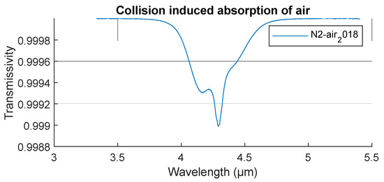
Figure 1.
Collision-induced absorption of air.
Line-by-line absorption data in Figure 1 was obtained from The HITRAN2016 molecular spectroscopic database [8] and converted to absorption coefficient spectrum using the MATLAB function Load Hitran by DeVore [26] for set individual gas component of a calculated number density. Within the nine molecular species presented in Table 2, a total of 25 isotopologs have been accounted for. An isotopolog is a variation of a molecule where at least one of its atoms are an isotope. Isotopologs of total molar concentrations of less than 0.01 ppm in dry air were omitted from the calculation. Abundance values were sourced from the HITRAN2016 database, whereas atomic masses of isotopes were obtained from Bievre et al. [27]. Absorption cross section of species is calculated for multiple isotopologs indexed with and weighted corresponding to isotopolog abundance .
The sum of abundance-weighted absorption cross sections of a molecular species is exported to numeric spectrum and multiplied by number density of the molecular species and path length . Note that constant gas species number densities were used upon exportation to include abundance data of all dry gases in one file, therefore correction factor is used afterwards—one for dry gases with presumably constant composition, and one for water vapor.
Number density, referring to the number of molecules in a unit of volume, is calculated using the gas law for real gases:
where is Avogadro’s constant, is amount of substance, is volume, is air pressure, is compressibility factor of air mixture (from Picard et al.’s CIPM-07 formulation [28] to compensate for its nonideal behavior), is molar fraction of water vapor in air, is the gas constant, and is the thermodynamic temperature of the gas mixture.
2.4. Compiling of the MATLAB Model
Compilation to numeric spectrum is possible using the Load Hitran function [26]; however, this task is highly computationally demanding, requiring up to several hours to complete at high resolution. An optimized version of this function would be desired for the purpose of repeated simulations.
The model can be computationally optimized by compiling the line-by-line data at reference parameter values, utilizing the Load Hitran function to obtain absorption coefficient spectrums of the dry air and the water vapor components, and subsequently adjusting the spectrums for the situational specific parameters. This two-part separation of calculations requires a single-time computationally demanding compilation and permits fast recall and adjustment of the saved data whenever the spectral transmissivity model is required.
It is important to point out that the described separation is not entirely theoretically correct. As temperature, partial and remaining pressure, and, thus, also water vapor concentration are influential parameters of the Load Hitran function, specifically influencing the pressure- and temperature-dependent Voigt line shape, each individual conversion of line-by-line data to numeric spectrum must theoretically be conducted at individual parameter values. While spectral line shift and broadening are theoretically present for parameter deviations, considering the relatively narrow range of expected atmospheric parameter values, the change in these effects can be minimized and neglected by setting reference parameters of the single-time compilation to expected usual values. Reference values are listed in Table 3.
Table 3.
Parameter set-point during spectrum preparation.
Separately, collision-induced cross sections of N2–air binary complexes, supplied by Hartmann [10] in the HITRAN CIA database, were simulated for the dry gas mixture.
The final algorithm of the MATLAB model for transmission spectrum calculation, with influential parameters of relative humidity, air pressure, and temperature, is displayed in Figure 2. The resulting MATLAB code produces spectral transmissivity of 1–18 µm for variable relative humidity, temperature, and atmospheric pressure, as influenced by number density of molecules. The program does not account for intrinsic line broadening and shift as an effect on particles due to variations in partial pressures and temperature. Final spectral transmissivity is plotted in Figure 3.

Figure 2.
Flow chart of air transmissivity calculation algorithm.

Figure 3.
Spectral transmissivity of air at various parameters. Pressure is set to 1013.25 hPa.
Total transmissivity of radiation of all wavelengths is displayed in Figure 4. Considering sensor spectral sensitivity, we use two different radiation thermometers in our laboratory. KT 19.01 II (SP01) measures in the spectral range of 2.0–2.7 µm and at temperatures between 350–2000 °C, and the Transfer Radiation Thermometer (TRT II) with ranges of 8–14 µm (SP82) for temperatures between −50–300 °C, and at 3.87 µm (SP41) for temperatures between 150–1000 °C.

Figure 4.
Total transmissivity of the black body radiation of wavelengths between 1 and 18 µm depending on relative humidity.
Spectral sensitivity characteristics, digitized from Heitronics pyrometer documentation [29] using WebPlotDigitizer [30] and imported into simulation environment, are displayed in Figure 5. Alongside these, generic vanadium oxide (VOx)-coated microbolometer spectral sensitivity by FLIR [31] was also imported, representing uncooled thermal imagers in the 8–14 µm range. Amplitude of each sensitivity curve is irrelevant, as the function fit of temperature vs. radiative power characteristic was calculated for each sensor individually.

Figure 5.
Relative spectral sensitivity of sensors.
Effects of the atmosphere at described settings are displayed in Figure 6. Transmissivities were calculated by simulating blackbody radiation, transmitted through atmosphere, and absorbed by the sensor of relative spectral sensitivity from Figure 5. Total transmissivity represents a fraction of the total radiation that is transmitted.

Figure 6.
Considering the sensor spectral sensitivity, (A) the effective transmissivity is plotted and (B) the calculated error of measurement due to the atmospheric transmissivity including radiation contribution at the set focal distance, air pressure 1013.25 hPa, and temperature 296 K for various relative humidity levels is plotted. The focal distance of the thermal imaging camera is adjustable and was set to 1 m.
Measurement errors were simulated by converting radiation, influenced by atmospheric absorption and emission over inverse radiation–temperature characteristic of the sensor, compiled for the black body source.
In accordance with the Beer–Lambert law (Equation (4)), one can adjust transmissivity to different path length by applying exponential correction factor to of path length .
Similarly, number density correction can be applied.
Considering that most pyrometers do not support transmissivity adjustments, correction must be applied manually, if necessary. Assuming equilibrium, where temperature of the environment is equal to temperature of the atmosphere in the radiation transfer path through the air, transmissivity factor can be applied to emissivity setting of the instrument using multiplication, considering that mathematical effect of these two parameters is equal. Furthermore, automatic compensation of emissivity is usually calculated using the temperature of radiation thermometer’s sensor inside the enclosure, which corresponds to the atmospheric temperature.
2.5. Comparison with Experimental Results
Practical influence on radiation thermometer was measured by Omejc [32], using a Vötsch VC7100 climatic chamber, where the radiation thermometer Heitronics KT19.01 II and radiation source FLUKE 4181 were positioned closely outside the chamber (Figure 7).

Figure 7.
Sketch of the validation experiment.
The manufacturer of the radiation source specifies emissivity of the flat-plate radiation thermometer calibrator at 0.95. In the experiment, the radiation transfer path included a 15 cm gap on the source side and extended through the climatic chamber openings, located 1.3 m apart. The diameter of the openings is 125 mm at the side of the radiation source and 50 mm at the other side, where the radiation thermometer was placed with neglectable gap. The experimental system was simulated using the compiled model of atmospheric spectral transmissivity by simulating two homogenous zones of gases, one within the chamber, with variable humidity and temperature of 23 °C, and one outside the chamber, between the opening and the radiation source, with heater-induced increased temperature (mean increase of 10% of total temperature difference) and ambient humidity of 30% RH. Instrumental emissivity setting was applied to the simulation to match the experimental setting. The systematical error of the radiation source from a postponed accuracy evaluation was included in the simulation; however with a time difference of over a year, possible drift error was not accounted for. Results of simulation of the experiment and measurements are presented in Figure 8.

Figure 8.
Comparison of experimental and simulated measurements. (A) The error represents measurement deviation from reference temperature and (B) the error represents discrepancy between the simulated measurement and actual measurement.
While the errors between simulation and measurement results could indicate incorrect behavior of the model, discrepancy between the results can at least partially be attributed to experiment realization uncertainty. For example, the size of the openings can locally distort the homogeneity of the climatic chamber, increasing the uncertainty of the experiment. The temperature outside the opening of the climatic chamber is also only approximated, introducing additional uncertainty to the simulation results.
3. Results
Results of sensor responses suggest that, amongst the instruments in use in the calibration laboratory practices, the effect of atmospheric interference is relatively high for the reference radiation thermometer Heitronics KT19.01 II and moderate for the low-temperature sensor on the Heitronics TRT II and vanadium oxide-based thermal cameras.
The constant offset between the results can be attributed to error in radiative temperature realization, whereas the measurement error appears to correlate between the simulation and the experiment, indicating correct behavior of the simulation-predicted sensitivity of at least the KT19.01 II radiation thermometer.
4. Discussion
Fractions of water vapor and CO2 mainly contribute to the spectral transmissivity of the air. Results of simulation reveal important atmospheric effects for some sensors, which need to be accounted for when calibrating and using these instruments for measurement. It is especially important in a practical calibration procedure of a radiation thermometer to account for influential parameters at atmospherically sensitive spectral ranges and to match atmospheric conditions during calibration as close as possible to the conditions in the target application (mainly moisture levels and the measurement distance). When conditions do not match with conditions of calibration, the calculated errors should either be taken into account for correction or included into the measurement uncertainty.
5. Conclusions
The sensitivity of the reference radiation thermometers KT19.01 II to atmospheric influential parameters is evidently high, therefore special attention needs to be paid to this thermometer during calibration and deployment.
Existing laboratory practice of listing permissible range of atmospheric parameters on the calibration certificate, which is relatively wide, is evidently not appropriate for this thermometer, as it significantly contributes to the calibration uncertainty, which was formerly underestimated.
To ensure the correct transfer of the reference temperature between the instrument calibration and deployment of the radiation thermometer as the reference for lower tier calibration traceability, matching, monitoring, documentation, and possible correction are necessary for the main influential parameters—measuring distance, relative humidity, atmospheric temperature, and pressure.
Further experimental research of atmospheric influences and comparison with the described model will be conducted in the future, by controlling the transfer path of calibration in front of the black body with the help of a climatic chamber with increased flow and better sealing at the radiation path openings.
Author Contributions
Conceptualization, V.M. and I.P.; methodology, V.M. and I.P.; software, V.M.; investigation, V.M. and I.P.; data curation, V.M.; writing—original draft preparation, V.M.; writing—review and editing, V.M. and I.P.; visualization, V.M.; supervision, I.P.; funding acquisition, I.P. All authors have read and agreed to the published version of the manuscript.
Funding
The authors acknowledge the financial support from the Slovenian Research Agency (research core funding No. P2-0225). The research was also supported partially by the Ministry of Economic Development and Technology, Metrology Institute of the Republic of Slovenia, in scope of contract 6401-18/2008/70 for the national standard laboratory for the field of thermodynamic temperature and humidity.
Data Availability Statement
The data presented in this study are available on request from the corresponding author. The data are not publicly available due to size restrictions.
Conflicts of Interest
The authors declare no conflict of interest.
References
- Elder, T.; Strong, J. The infrared transmission of atmospheric windows. J. Frankl. Inst. 1953, 255, 189–208. [Google Scholar] [CrossRef]
- Wyatt, P.J.; Stull, V.R.; Plass, G.N. The Infrared Transmittance of Water Vapor. Appl. Opt. 1964, 3, 229–241. [Google Scholar] [CrossRef]
- Burch, D.E.; Singleton, E.B.; France, W.L.; Williams, D. Infrared Absorption by Carbon Dioxide, Water Vapor, and Minor Atmospheric Constituents; The Ohio State University Research Foundation: Cambridge, MA, USA, 1960. [Google Scholar]
- Zhang, H.; Wang, C.; Li, X.; Sun, B.; Jiang, D. Design and Implementation of an Infrared Radiant Source for Humidity Testing. Sensors 2018, 18, 3088. [Google Scholar] [CrossRef] [PubMed]
- Kneizys, F.X.; Shettle, E.P.; Abreu, L.W.; Chetwynd, J.H.; Anderson, G.P.; Gallery, W.O.; Selby, J.E.A.; Clough, S.A. Users Guide to LOWTRAN 7; U.S. Government Printing Office: Hanscom, MA, USA, 1988. [Google Scholar]
- Kneizys, F.X.; Abreu, L.W.; Shettle, E.P.; Chetwynd, J.H.; Anderson, G.P.; Berk, A.; Bernstein, L.S.; Robertson, D.C.; Acharya, P.; Rothman, L.S.; et al. The MODTRAN 2/3 Report and LOWTRAN 7 MODEL; Ontar Corp.: North Andover, MA, USA, 1996. [Google Scholar]
- Chen, X.; Wei, H. A Combined Atmospheric Radiative Transfer Model (CART): A Review and Applications. J. Opt. Soc. Korea 2010, 14, 190–198. [Google Scholar] [CrossRef]
- Gordon, I.E.; Rothman, L.S.; Hill, C.; Kochanov, R.V.; Tan, Y.; Bernath, P.F.; Birk, M.; Boudon, V.; Campargue, A.; Chance, K.V.; et al. The HITRAN2016 molecular spectroscopic database. J. Quant. Spectrosc. Radiat. Transf. 2017, 203, 3–69. [Google Scholar] [CrossRef]
- Karman, T.; Gordon, I.E.; van der Avoird, A.; Baranov, Y.I.; Boulet, C.; Drouin, B.J.; Groenenboom, G.C.; Gustafsson, M.; Hartmann, J.-M.; Kurucz, R.L.; et al. Update of the HITRAN collision-induced absorption section. Icarus 2019, 328, 160–175. [Google Scholar] [CrossRef]
- Hartmann, J.M.; Boulet, C.; Toon, G.C. Collision-induced absorption by N2 near 2.16 μm: Calculations, model and consequences for atmospheric remote sensing. J. Geophys. Res. Atmos. 2019, 122, 2419–2428. [Google Scholar] [CrossRef]
- Picard, A.; Davis, R.; Gläser, M.; Fujii, K. Revised formula for the density of moist air (CIPM-2007). Metrologia 2008, 45, 149–155. [Google Scholar] [CrossRef]
- Hardy, B. ITS-90 formulations for vapor pressure, frostpoint temperature, dewpoint temperature, and enhancement factors in the range −100 to +100 C. In Proceedings of the Third International Symposium on Humidity & Moisture, Teddington, London, UK, 6 April 1998. [Google Scholar]
- Krogh, A. The Composition of the Atmosphere; Royal Danish Academy of Sciences and Letters: Copenhagen, Denmark, 1919; Volume 12. [Google Scholar]
- Paneth, F.A. The chemical composition of the atmosphere. Q. J. R. Meteorol. Soc. 1937, 63, 433–443. [Google Scholar] [CrossRef]
- Giacomo, P. Equation for the Determination of the Density of Moist Air. Metrologia 1982, 18, 33–40. [Google Scholar] [CrossRef]
- Keeling, R.F. Measuring correlations between atmospheric oxygen and carbon dioxide mole fractions: A preliminary study in urban air. J. Atmos. Chem. 1988, 7, 153–176. [Google Scholar] [CrossRef]
- Gatley, D.P.; Herrmann, S.; Kretzschmar, H.-J. A Twenty-First Century Molar Mass for Dry Air. HVAC&R Res. 2008, 14, 655–662. [Google Scholar] [CrossRef]
- Ginzburg, A.S.; Vinogradova, A.A.; Fedorova, E.I.; Nikitich, E.V.; Karpov, A.V. Content of oxygen in the atmosphere over large cities and respiratory problems. Izv. Atmos. Ocean. Phys. 2014, 50, 782–792. [Google Scholar] [CrossRef]
- Park, S.Y.; Kim, J.S.; Lee, J.B.; Esler, M.B.; Davis, R.S.; Wielgosz, R.I. A redetermination of the argon content of air for buoyancy corrections in mass standard comparisons. Metrologia 2004, 41, 387–395. [Google Scholar] [CrossRef]
- Schlatter, T. Atmospheric Composition and Vertical Structure. Environ. Impact Manuf. 2009, 6, 1–54. [Google Scholar]
- Dlugokencky, E. NOAA/GML. 4 May 2021. Available online: https://www.esrl.noaa.gov/gmd/ccgg/trends/global.html (accessed on 26 March 2021).
- United States Environmental Protection Agency. Status and Trends of Key Air Pollutants. 2019. Available online: https://www.epa.gov/air-trends (accessed on 6 May 2021).
- Williams, D.R. NASA Earth Fact Sheet. NASA Goddart Space Flight Center. 25 November 2020. Available online: https://nssdc.gsfc.nasa.gov/planetary/factsheet/earthfact.html (accessed on 26 March 2021).
- Sedunov, J.S.; Avdjushin, S.I.; Borisenkov, E.P.; Volkovickij, O.A.; Petrov, N.N.; Rejtenbah, R.G.; Smirnov, V.I.; Chernikov, A.A. Spravochnik (Spravochnye Dannye, Modeli) [The Atmosphere: A Handbook (Reference Data and Models)]; Gidrometeoizdat: Sankt Petersburg, Russia, 1991. [Google Scholar]
- COESA. U.S. Standard Atmosphere, 1962; U.S. Government Printing Office: Washington, DC, USA, 1962. [Google Scholar]
- DeVore, P.T.S. Load HITRAN 2004+ Data. 23 May 2014. Available online: https://www.mathworks.com/matlabcentral/fileexchange/45819-load-hitran-2004-data (accessed on 26 March 2021).
- De Bievre, P.; Gallet, M.; Holden, N.E.; Barnes, I.L. Isotopic Abundances and Atomic Weights of the Elements. J. Phys. Chem. Ref. Data 1984, 13, 809–891. [Google Scholar] [CrossRef]
- Picard, A.; Fang, H.; Glaser, M. Discrepancies in air density determination between the thermodynamic formula and a gravimetric method: Evidence for a new value of the mole fraction of argon in air. Metrologia 2004, 41, 396–400. [Google Scholar] [CrossRef]
- Heitronics Infrarot Messtechnik GmbH. Infrared Radiation Pyrometer KT19 II Operation Instructions; Heitronics Infrarot Messtechnik GmbH: Wiesbaden, Germany, 2002. [Google Scholar]
- Rohatgi, A. WebPlotDigitizer: Version 4.4. 2020. Available online: https://automeris.io/WebPlotDigitizer/ (accessed on 17 May 2021).
- Teledyne FLIR, LLC. What Is the Typical Spectral Response for Certain Camera/Lens Combination? Available online: https://www.flir.com/support-center/Instruments/what-is-the-typical-spectral-response-for-certain-cameralens-combination/ (accessed on 26 March 2021).
- Omejc, J. Vpliv Relativne Vlažnosti na Kazanje Sevalnih Termometrov [Influence of relative humidity on radiation thermometer measurements]. Diploma Thesis, Univerza v Ljubljani, Ljubljana, Slovenia, 2020. [Google Scholar]


Publisher’s Note: MDPI stays neutral with regard to jurisdictional claims in published maps and institutional affiliations. |
© 2021 by the authors. Licensee MDPI, Basel, Switzerland. This article is an open access article distributed under the terms and conditions of the Creative Commons Attribution (CC BY) license (https://creativecommons.org/licenses/by/4.0/).