
Energy Management Strategy of a Hybrid Power System Based on V2X Vehicle Speed Prediction


Abstract
:1. Introduction
2. Hybrid Power Drive Train Modeling
2.1. Hybrid Vehicle Model
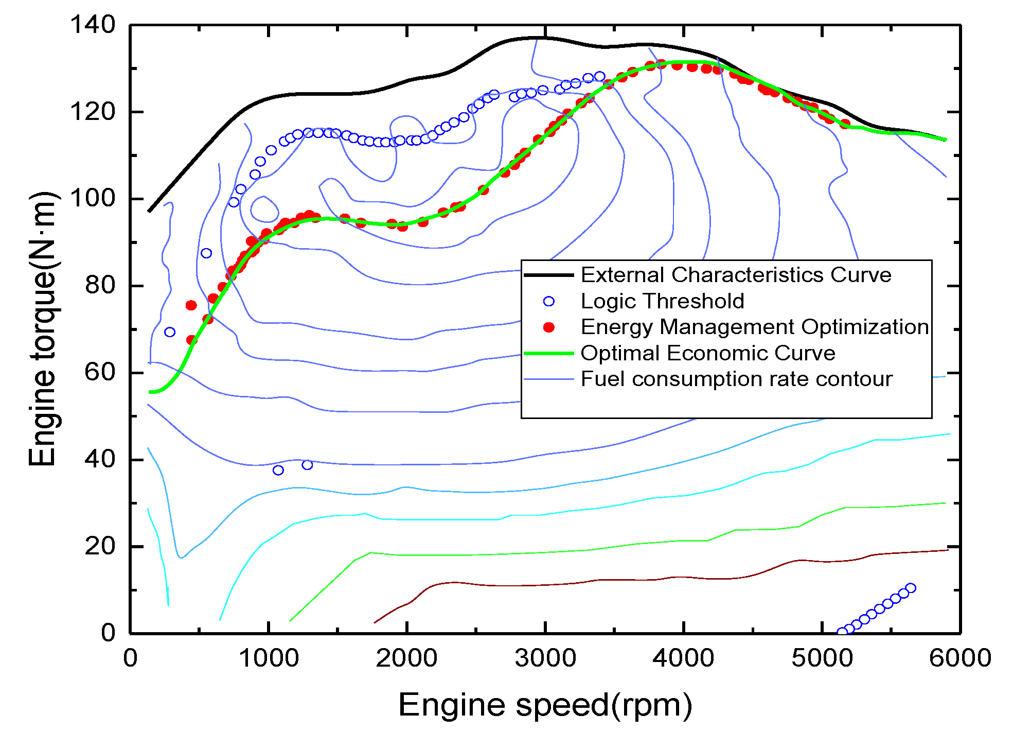
2.1.1. Engine Model
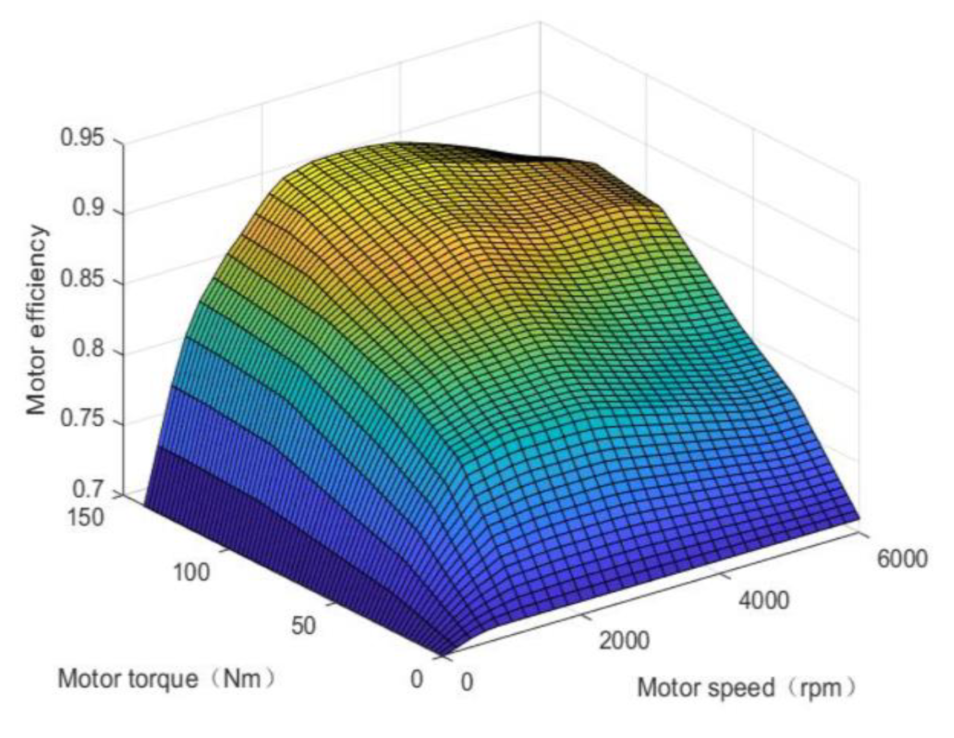
2.1.2. Motor Model
2.1.3. Battery Model
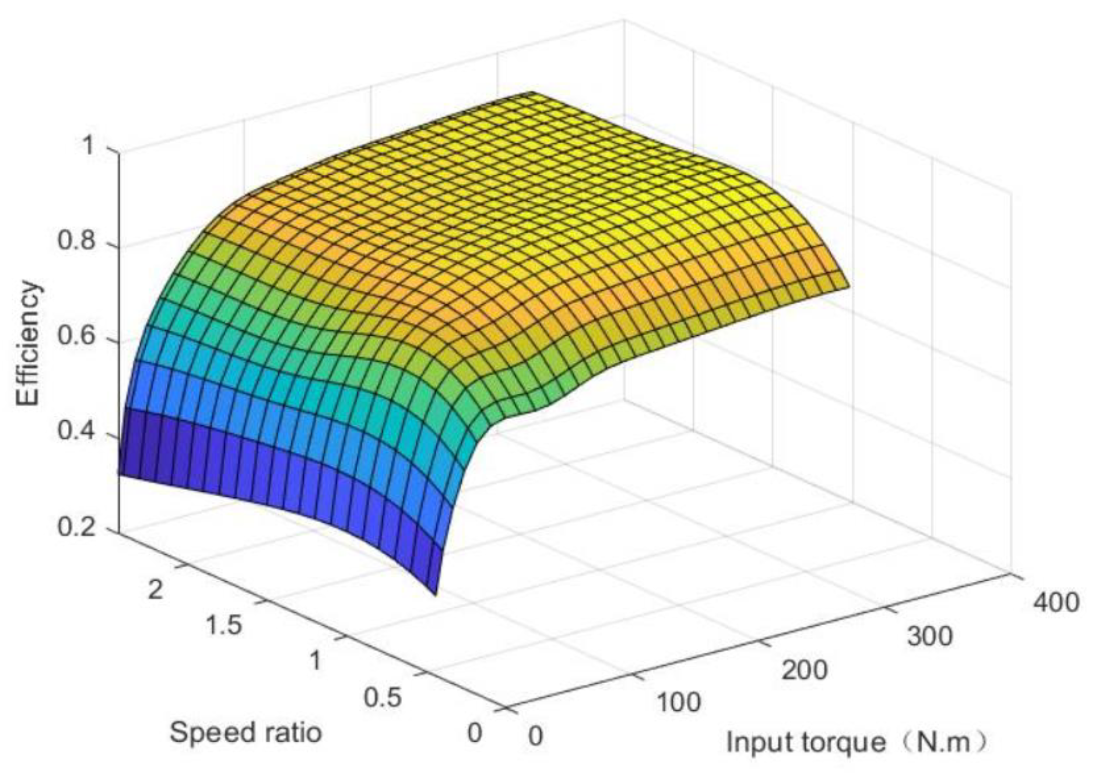
2.1.4. Transmission Model
2.1.5. Whole Vehicle Model
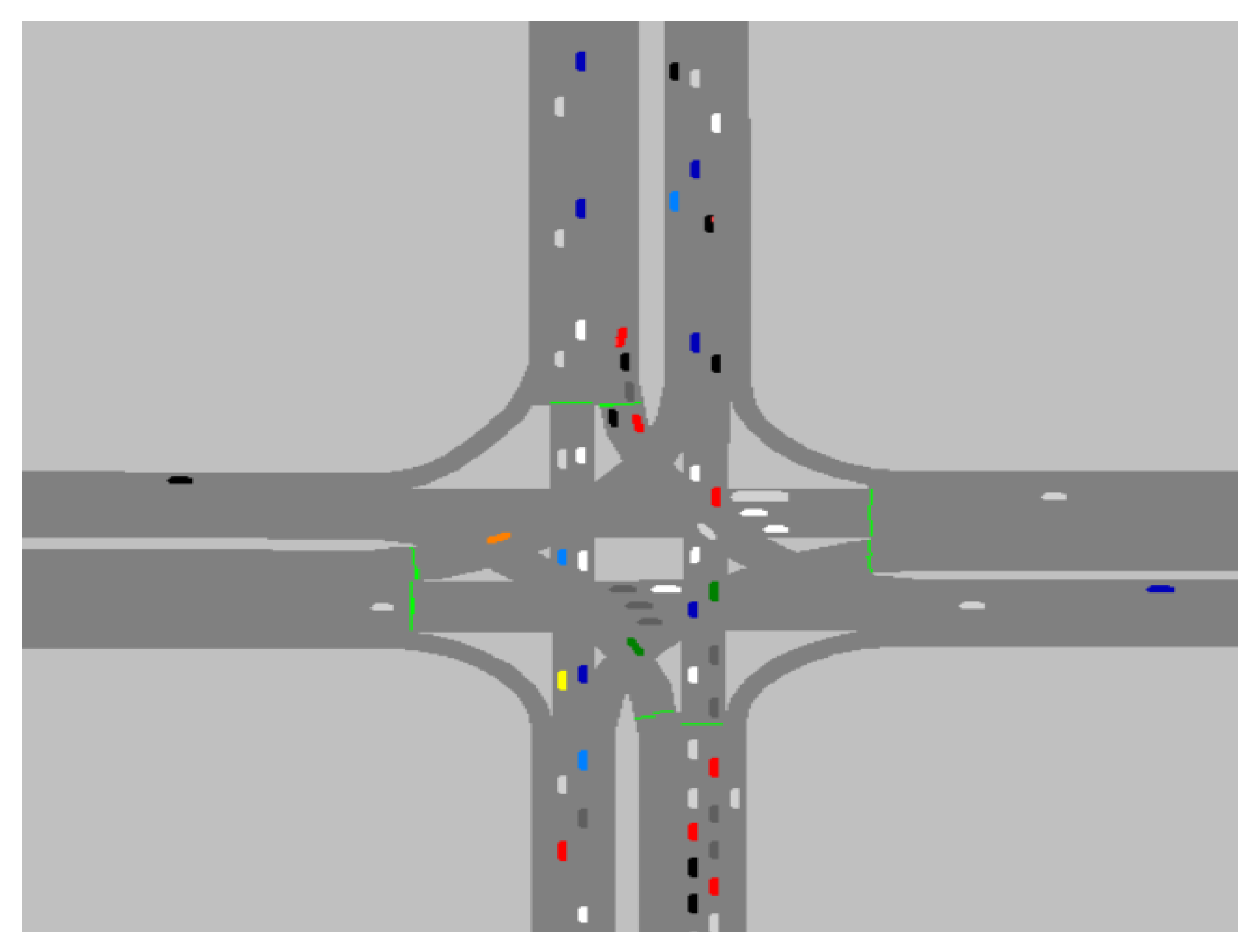
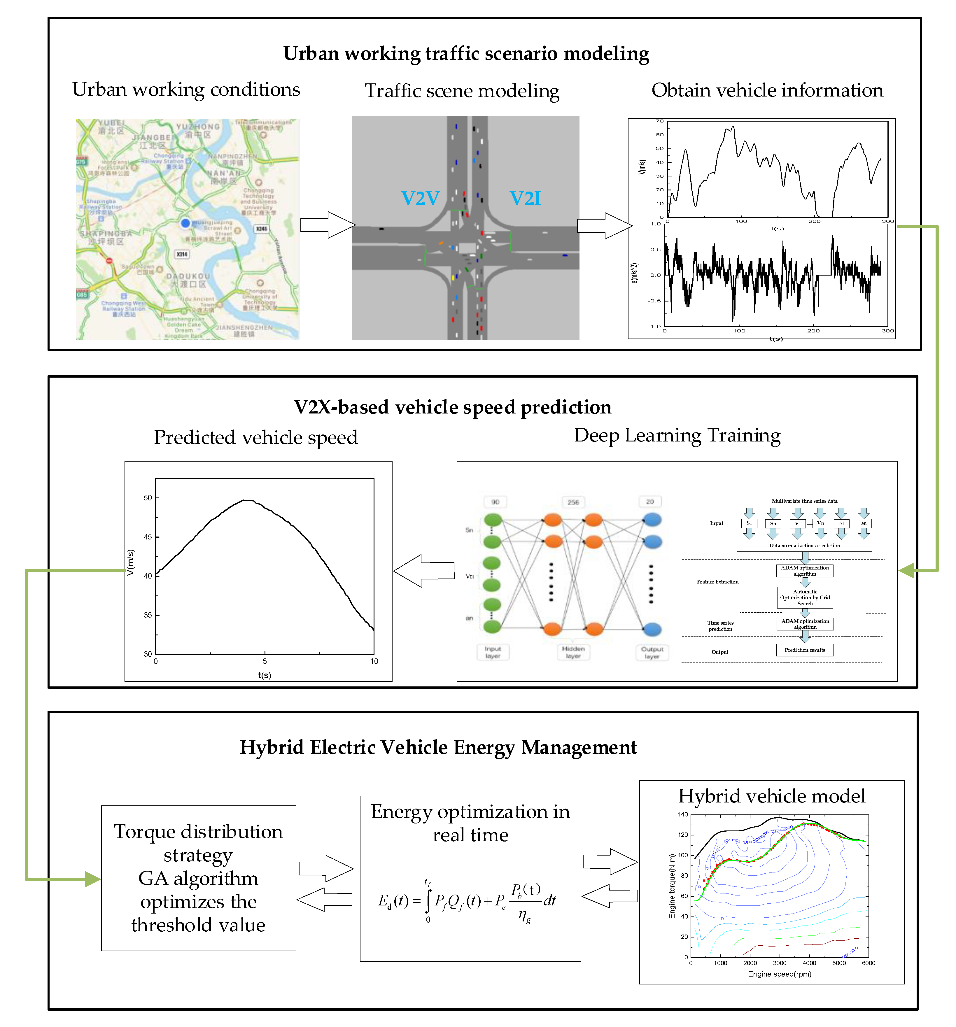
2.2. Traffic Model
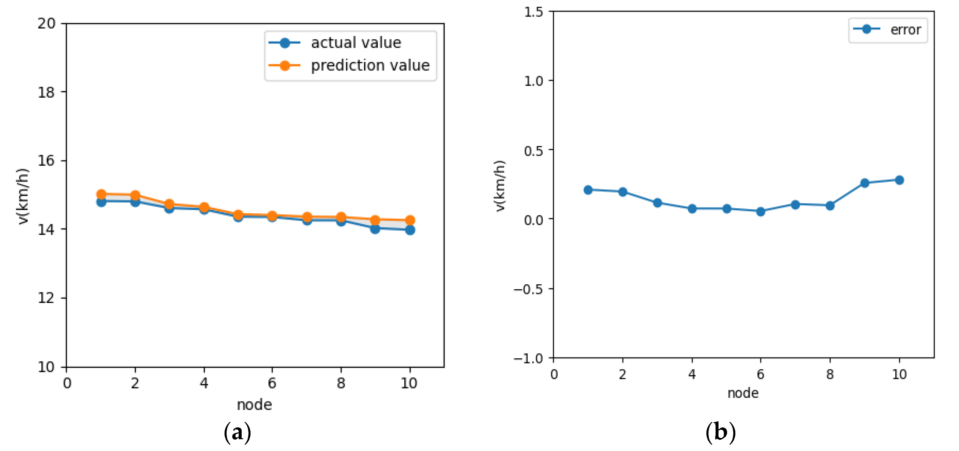
3. Vehicle Speed Prediction
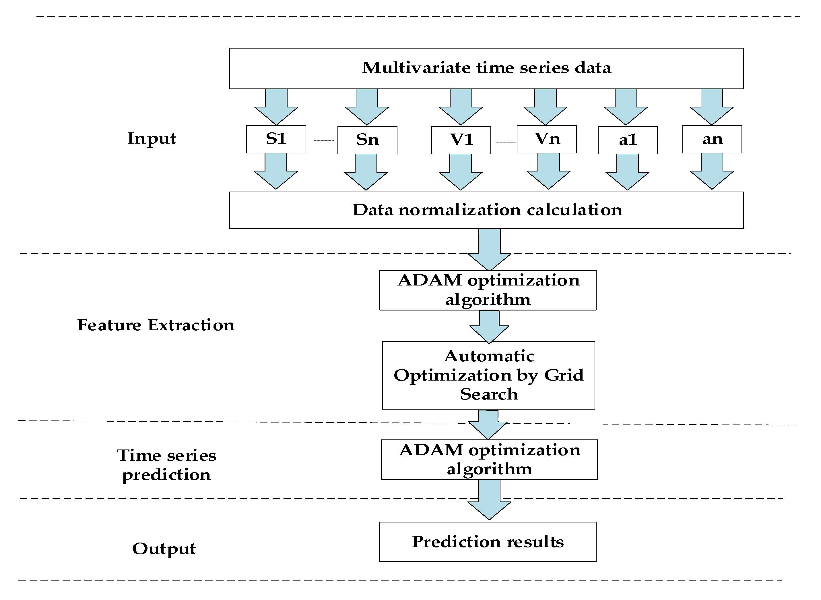
3.1. Vehicle Speed Prediction Model Architecture
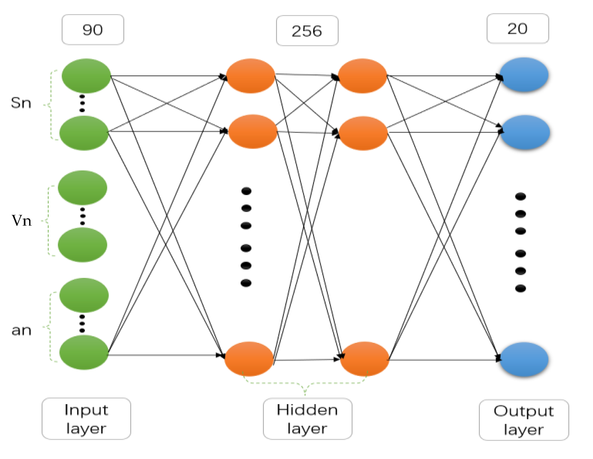
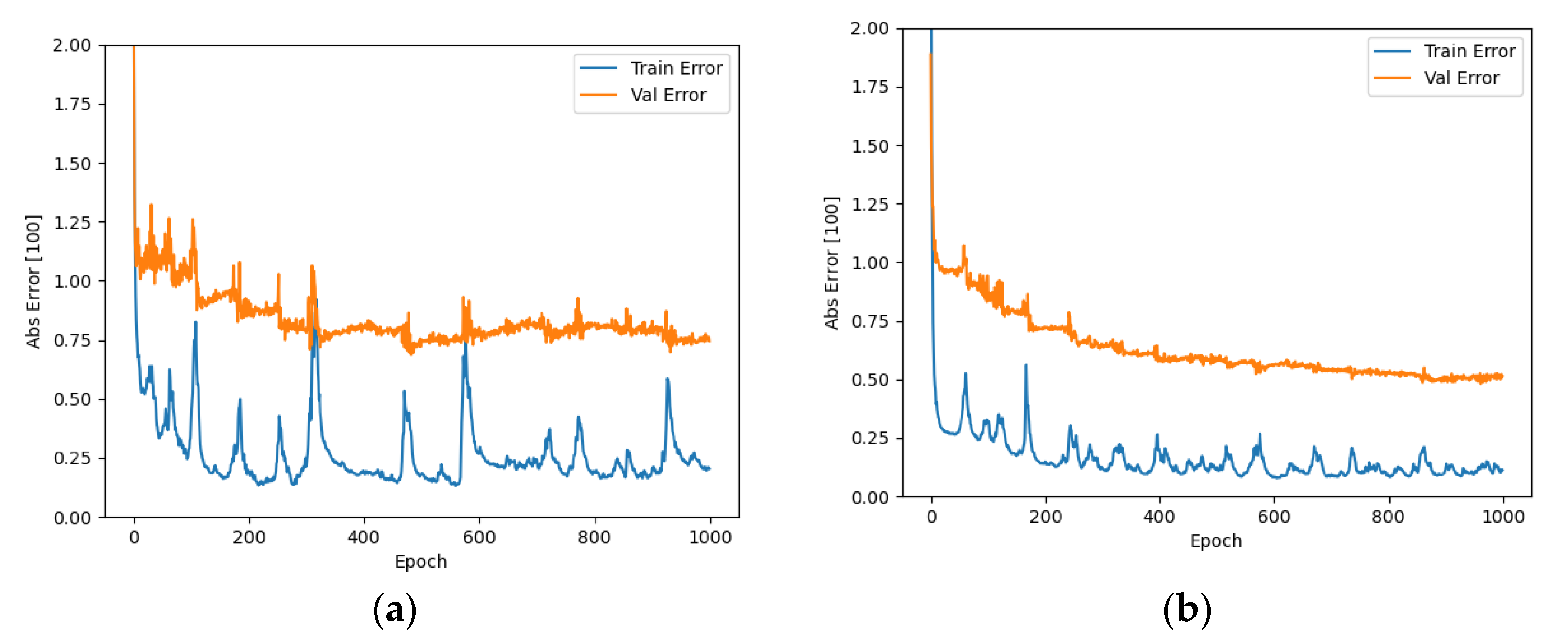
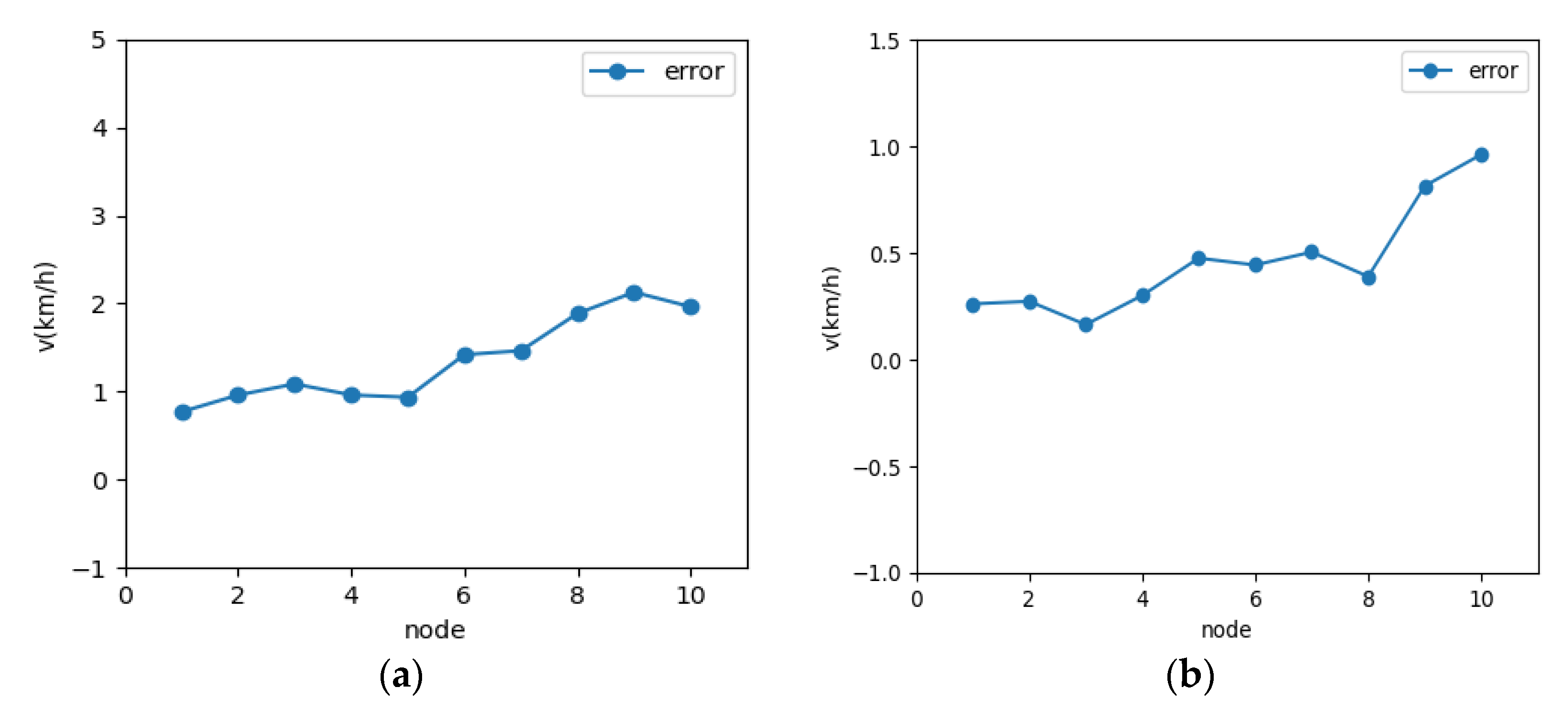
3.2. Deep Learning Network
4. Real-Time Optimized Energy Management Algorithm
4.1. Evaluation of Energy Consumption Economy of Plug-In Hybrid Electric Vehicles
4.2. Energy Management Control Strategy
4.3. The Proposed Real-Time Energy Management
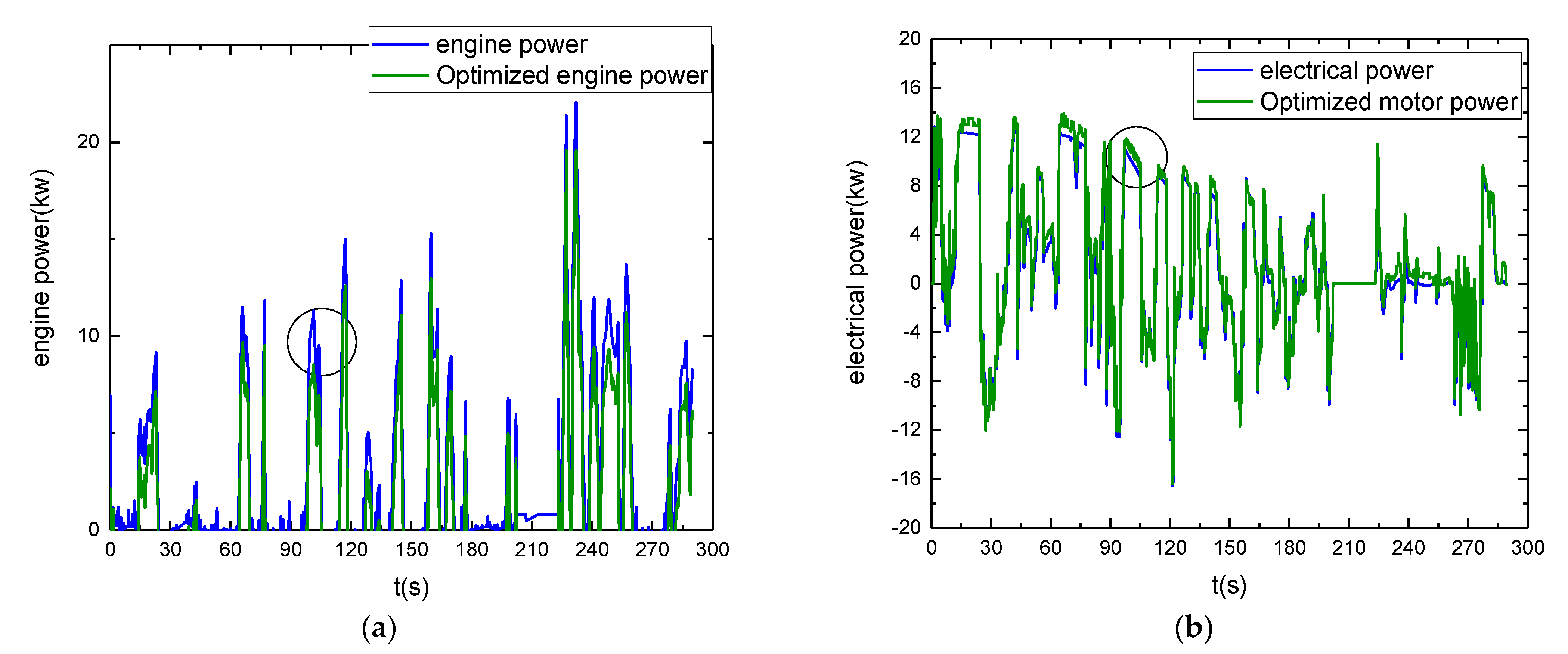
5. Analysis of Simulation Results
Optimization Results and Analysis
6. Conclusions
Author Contributions
Funding
Institutional Review Board Statement
Informed Consent Statement
Data Availability Statement
Conflicts of Interest
References
- Hong, J.L.; Gao, B.Z.; Dong, S.Y.; Cheng, Y.F.; Wang, Y.H.; Chen, H. Key Problems and Research Progress of Energy Saving Optimization for Intelligent Connected Vehicles. China J. Highw. Transp. 2021, 1, 51. [Google Scholar]
- Yuan, H.T.; Zhao, H.; Pan, G.C.; Chou, J.Z. A research on predictive ground speed of hybrid electric vehicle based on Markov. Intell. City 2021, 7, 18–22. [Google Scholar]
- Chen, F.; Yin, Z.; Ye, Y.; Sun, D. Taxi hailing choice behavior and economic benefit analysis of emission reduction based on multi-mode travel big data. Transp. Policy 2020, 97, 73–84. [Google Scholar] [CrossRef]
- Zhang, L.; Liu, W.; Qi, B. Energy optimization of multi-mode coupling drive plug-in hybrid electric vehicles based on speed prediction. Energy 2020, 206, 118–126. [Google Scholar] [CrossRef]
- Hu, X.; Liu, T.; Qi, X.; Barth, M. Reinforcement Learning for Hybrid and Plug-In Hybrid Electric Vehicle Energy Management. Recent Advances and Prospects. IEEE Ind. Electron. Mag. 2019, 13, 16–25. [Google Scholar] [CrossRef] [Green Version]
- Pan, L.S.; Gao, J.P.; Song, Z.; Hao, J.G. Vehicle Speed Prediction Method Based on Multi-source Information Fusion and Vehicle Energy Management. J. Henan Univ. Sci. Technol. (Nat. Sci.) 2020, 41. [Google Scholar] [CrossRef]
- Yang, Y.L.; Shi, X.F. Driving Cycle Prediction Energy Management Strategy of Series-Parallel Hybrid Electric Vehicles. Mach. Design Manuf. 2020, 10, 276–280. [Google Scholar]
- Li, Z. Optimization of fuel cost using transit green-speed guidance strategy. J. Transp. Sci. Eng. 2015, 31, 68–74. [Google Scholar]
- Yang, M.Y.; Lou, T.; Li, Y.F. Research on Future Vehicle Speed Prediction Model on Roads. J. Chin. Comput. Syst. 2018, 39, 2748–2752. [Google Scholar]
- Wen, B.X.; Wang, W.D.; Xiang, C.L.; Zhao, Y.L. Torque coordinated control for the multi power in parallel-series HEV. J. Harbin Inst. Technol. 2016, 48, 72–79. [Google Scholar]
- Zhai, Y.; Yu, J.D.; Chen, S.S.; Chen, X. Research on Modeling and Simulation of Vector Control System for Permanent Magnet Synchronous Motor. Wirel. Commun. Technol. 2019, 28, 23–27. [Google Scholar]
- Lin, N.; Zong, C.; Shi, S. The Method of Mass Estimation Considering System Error in Vehicle Longitudinal Dynamics. Energies 2018, 12, 52. [Google Scholar] [CrossRef] [Green Version]
- Han, S.J.; Zhang, F.Q.; Ren, Y.F.; Xi, J.Q. Predictive Energy Management Strategies in Hybrid Electric Vehicles Using Hybrid Deep Learning Networks. China J. Highw. Transp. 2020, 33, 1–9. [Google Scholar]
- Zhang, F.Q.; Xi, J.Q.; Langari, R. Real-Time Energy Management Strategy Based on Velocity Forecasts Using V2V and V2I Communications. IEEE Trans. Intell. Transp. Syst. 2017, 18, 416–430. [Google Scholar] [CrossRef]
- Zhang, F.Q. The Control Strategy Optimization of Parallel Hybrid Electric Vehicle Using Vehicle-to-Vehicle (V2V) Communication and Vehicle-to-Infrastructure (V2I) Communication. Ph.D. Thesis, Beijing Institute of Technology, Beijing, China, 2016. [Google Scholar]
- Lu, S.Q.; Huang, Z.X. Prediction model of short-term traffic flow based on CNN-GRU deep learning. J. Transp. Sci. Eng. 2020, 3, 74–80. [Google Scholar]
- Pei, J.Z.; Su, Y.X.; Zhang, D.H.; Qi, Y.; Leng, Z.W. Velocity forecasts using a combined deep learning model in hybrid electric vehicles with V2V and V2I communication. Sci. China Technol. Sci. 2020, 63, 55–64. [Google Scholar] [CrossRef]
- Zeng, Y.P.; Qin, D.T.; Su, L.; Yao, M.Z. Fuel Consumption and Emission Multi-objective Parameter Optimization for the Powertrain of a Plug-in HE. Automot. Eng. 2016, 38, 397–402, 434. [Google Scholar]
- Dong, Y.Q.; Wu, H.B.; Zhou, J.B.; Xu, S.C. Fuzzy Energy Management Strategy of PHEV Based on Genetic Algorithm. Optim. J. Jiamusi Univ. (Nat. Sci. Ed.) 2021, 39, 121–125. [Google Scholar]


| Part | Parameter | Value |
|---|---|---|
| Vehicle | Vehicle mass m/kg | 1350 |
| Windward area A/m2 | 2.28 | |
| Air resistance coefficient Cd | 0.32 | |
| Wheel radius r/m | 0.295 | |
| Tire rolling resistance coefficient fr | 0.0135 | |
| Engine | Maximum power Pemax/kw | 68 |
| Maximum torque Temax/(N·M) | 137 | |
| Rotational speed /(r·min−1) | 800–6000 | |
| Motor | Maximum power Pmmax/kw | 60 |
| Maximum torque Tmmax/(N·M) | 140 | |
| Rotational speed /(r·min−1) | 0–6000 | |
| Battery | Capacity Q/(A·h) | 40 |
| Nominal voltage U/V | 336 | |
| CVT | Speed ratio icvt | 0.422–2.432 |
| Main reduction ratio | 5.24 |
| Number of Hidden Layers | Number of Nodes per Layer | Learning Rate | Number of Iterations | RMSE |
|---|---|---|---|---|
| 2 | 256 | 0.1 | 100 | 0.056996938 |
| 2 | 64 | 0.001 | 1000 | 0.095363609 |
| 2 | 64 | 0.1 | 1000 | 0.095460914 |
| 1 | 512 | 0.0001 | 1000 | 0.097611815 |
| 1 | 256 | 0.001 | 1000 | 0.101234831 |
| 2 | 512 | 0.1 | 100 | 0.103126287 |
| 3 | 512 | 0.0001 | 100 | 0.111647338 |
| 1 | 8 | 0.0001 | 10 | 1.444064856 |
| 1 | 8 | 0.01 | 10 | 1.470003366 |
| 1 | 8 | 0.1 | 10 | 1.497559309 |
| Mode | Conditions | Torque Distribution |
|---|---|---|
| CD Electric drive | ||
| CD Hybrid drive | Instant Advantage Search | |
| CS Electric drive | ||
| CS Engine drive | ||
| CS Hybrid drive | Instant Advantage Search | |
| Charging | ||
| Brake Recovery |
| Performance Parameters | Fuel Consumption L/100 km | Electricity Consumption kwh/100 km | Energy Economy (CNY) | Economic Improvement (%) | CO2 Emissions (g/km) | CO2 Emissions Reduction (%) |
|---|---|---|---|---|---|---|
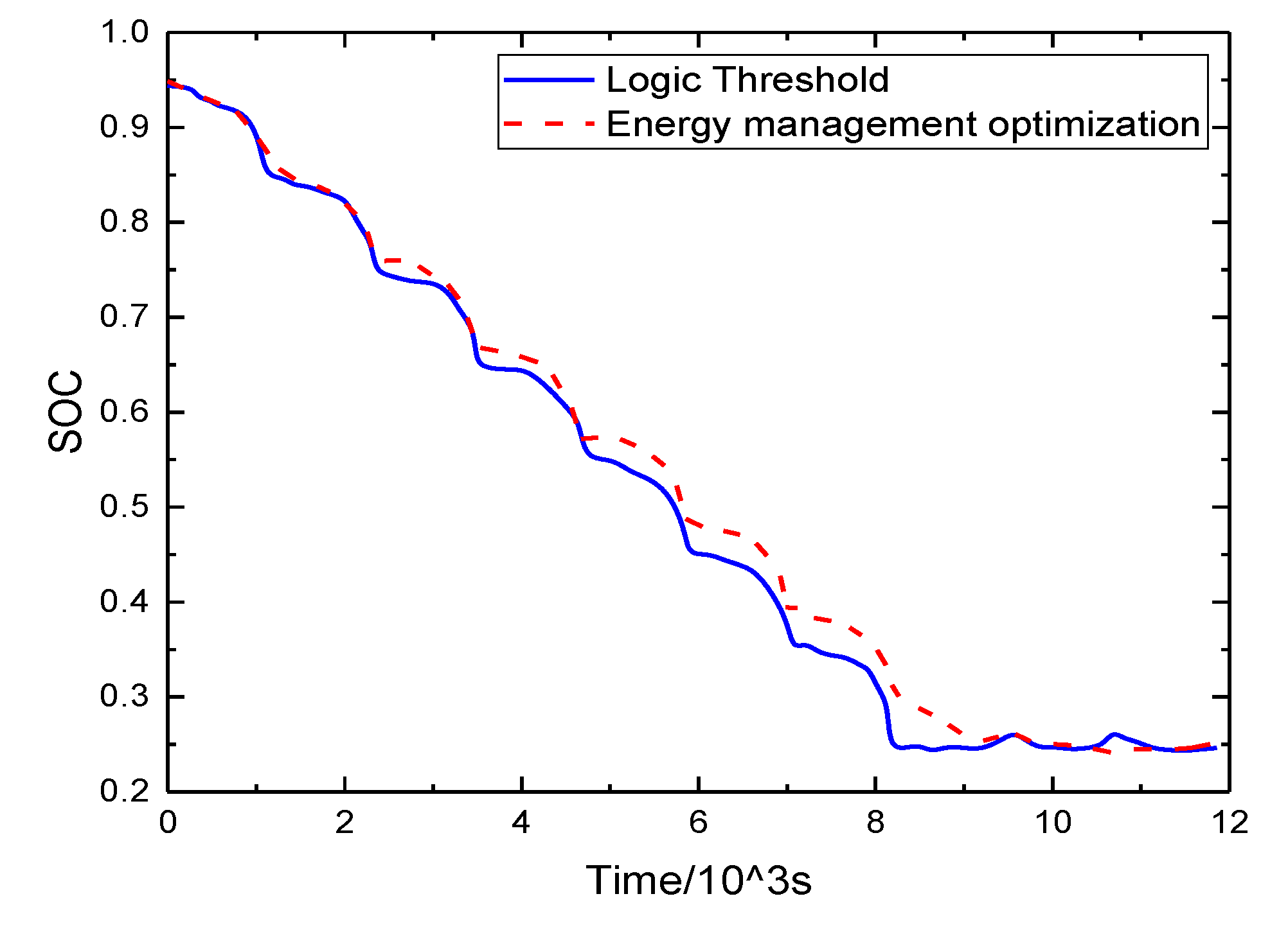
| Based on logical thresholds | 2.82 | 3.78 | 20.35 | - | 68.64 | - |
| Based on logic threshold with transient optimization | 2.27 | 5.42 | 17.7 | 13.02 | 57.63 | 16.04 |
Publisher’s Note: MDPI stays neutral with regard to jurisdictional claims in published maps and institutional affiliations. |
© 2021 by the authors. Licensee MDPI, Basel, Switzerland. This article is an open access article distributed under the terms and conditions of the Creative Commons Attribution (CC BY) license (https://creativecommons.org/licenses/by/4.0/).
Share and Cite
Ye, M.; Chen, J.; Li, X.; Ma, K.; Liu, Y. Energy Management Strategy of a Hybrid Power System Based on V2X Vehicle Speed Prediction. Sensors 2021, 21, 5370. https://doi.org/10.3390/s21165370
Ye M, Chen J, Li X, Ma K, Liu Y. Energy Management Strategy of a Hybrid Power System Based on V2X Vehicle Speed Prediction. Sensors. 2021; 21(16):5370. https://doi.org/10.3390/s21165370
Chicago/Turabian StyleYe, Ming, Jing Chen, Xu Li, Kai Ma, and Yonggang Liu. 2021. "Energy Management Strategy of a Hybrid Power System Based on V2X Vehicle Speed Prediction" Sensors 21, no. 16: 5370. https://doi.org/10.3390/s21165370
APA StyleYe, M., Chen, J., Li, X., Ma, K., & Liu, Y. (2021). Energy Management Strategy of a Hybrid Power System Based on V2X Vehicle Speed Prediction. Sensors, 21(16), 5370. https://doi.org/10.3390/s21165370