
Vehicle Localization Using 3D Building Models and Point Cloud Matching

 ,
,  , , and
Abstract
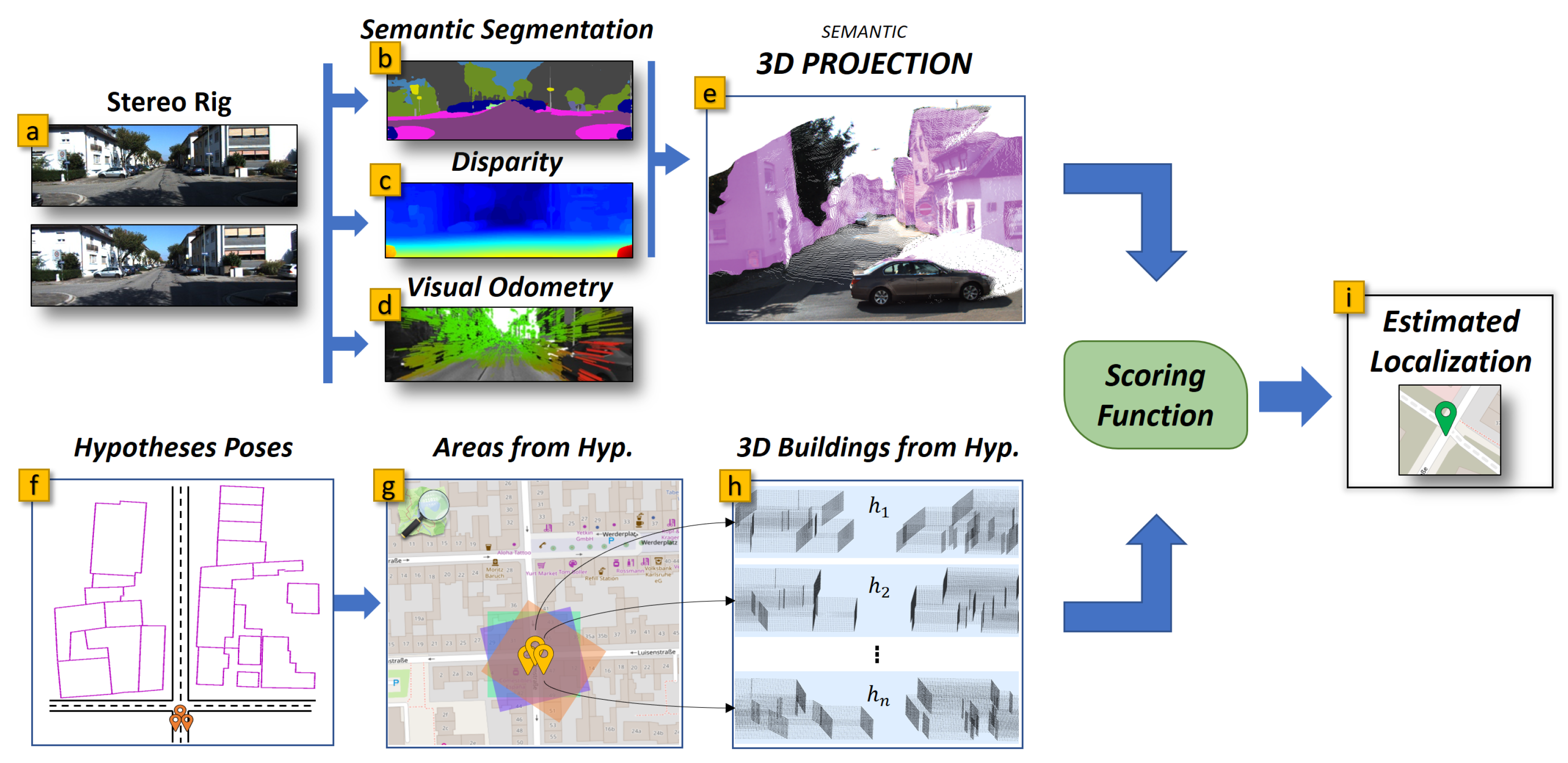
:1. Introduction
- A revised façades detection pipeline that uses pre-trained Deep neural network(DNNs) for 3D reconstruction and pixel-level semantic segmentation;
- The 3D structure of the perceived buildings is used by the matching process, differently from our previous work, which approximated the façades by fitting infinite planes;
- A new particle scoring method that uses the GICP registration technique [14] to estimate the likelihood of the observation, i.e., of the perceived buildings, with respect to the OSM data.
2. Related Work
- A 3D stereo reconstruction phase using the Semi-global block matching (SGBM) algorithm available in the OpenCV library [33];
- A 3D preprocessing stage aimed at refining the noisy data produced with SGBM and surface normal computation;
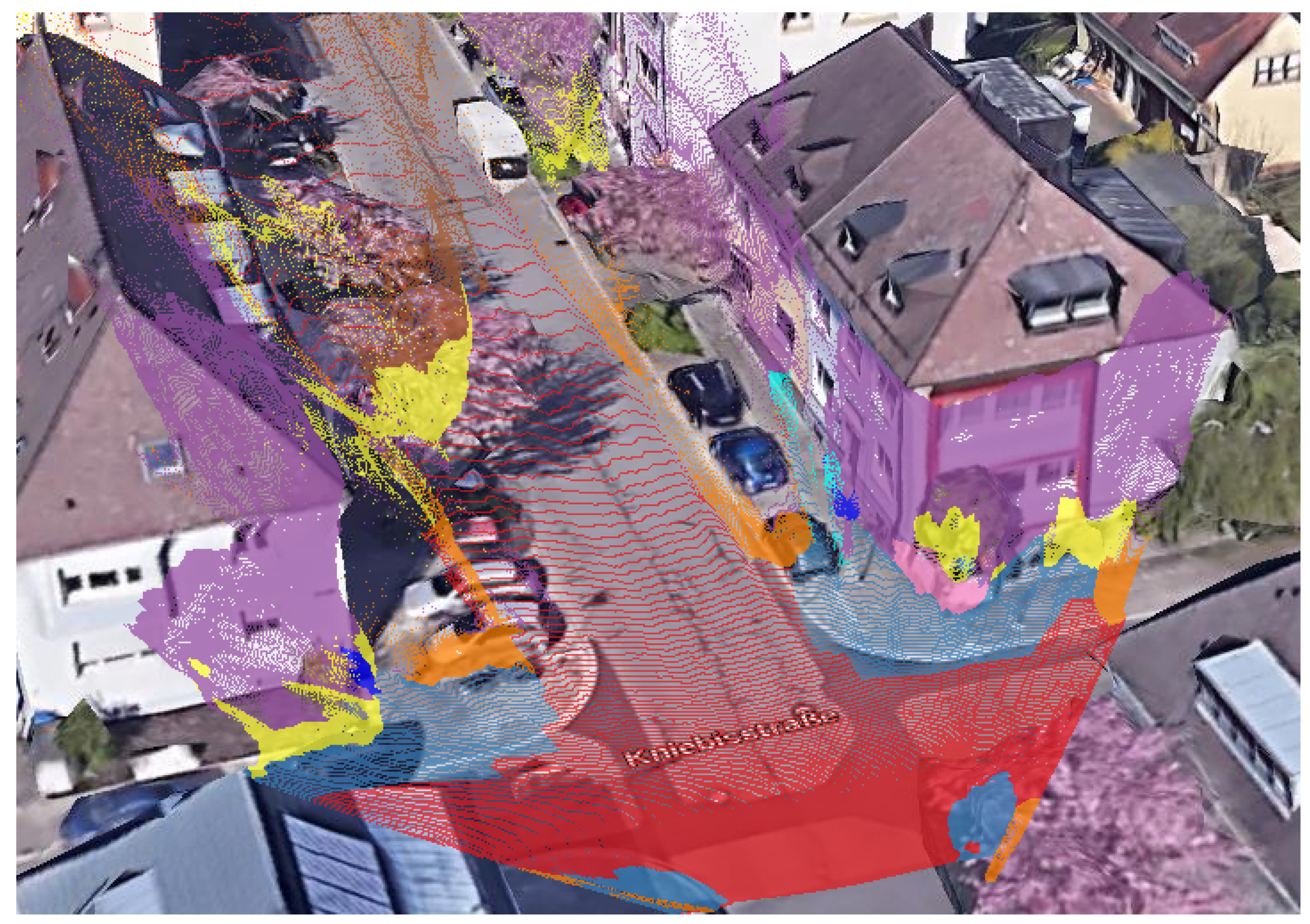
- A façade detection phase, involving the region growing segmentation algorithm implemented within the PCL library, followed by a clustering phase on the resulting 3D point cloud;
- A model fitting phase in which we took into consideration only regions perpendicular to the road surface;
- The extraction of the buildings’ outlines from the OpenStreetMap database;
- Finally, a step during which we compare the buildings’ outlines with the detected façades.
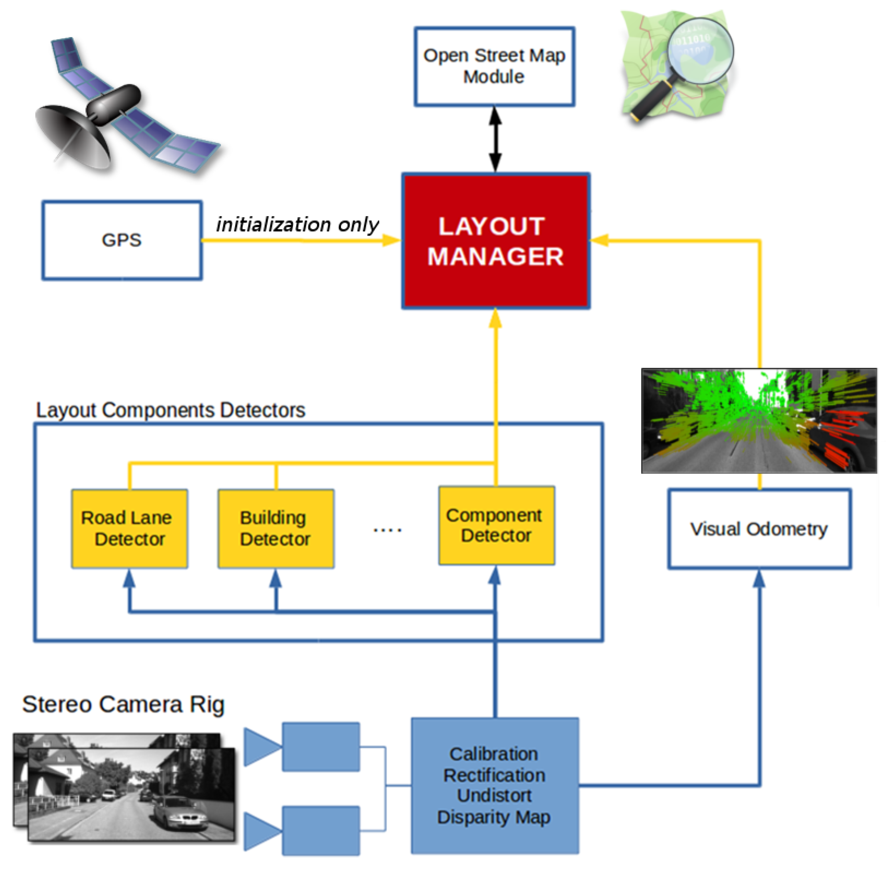
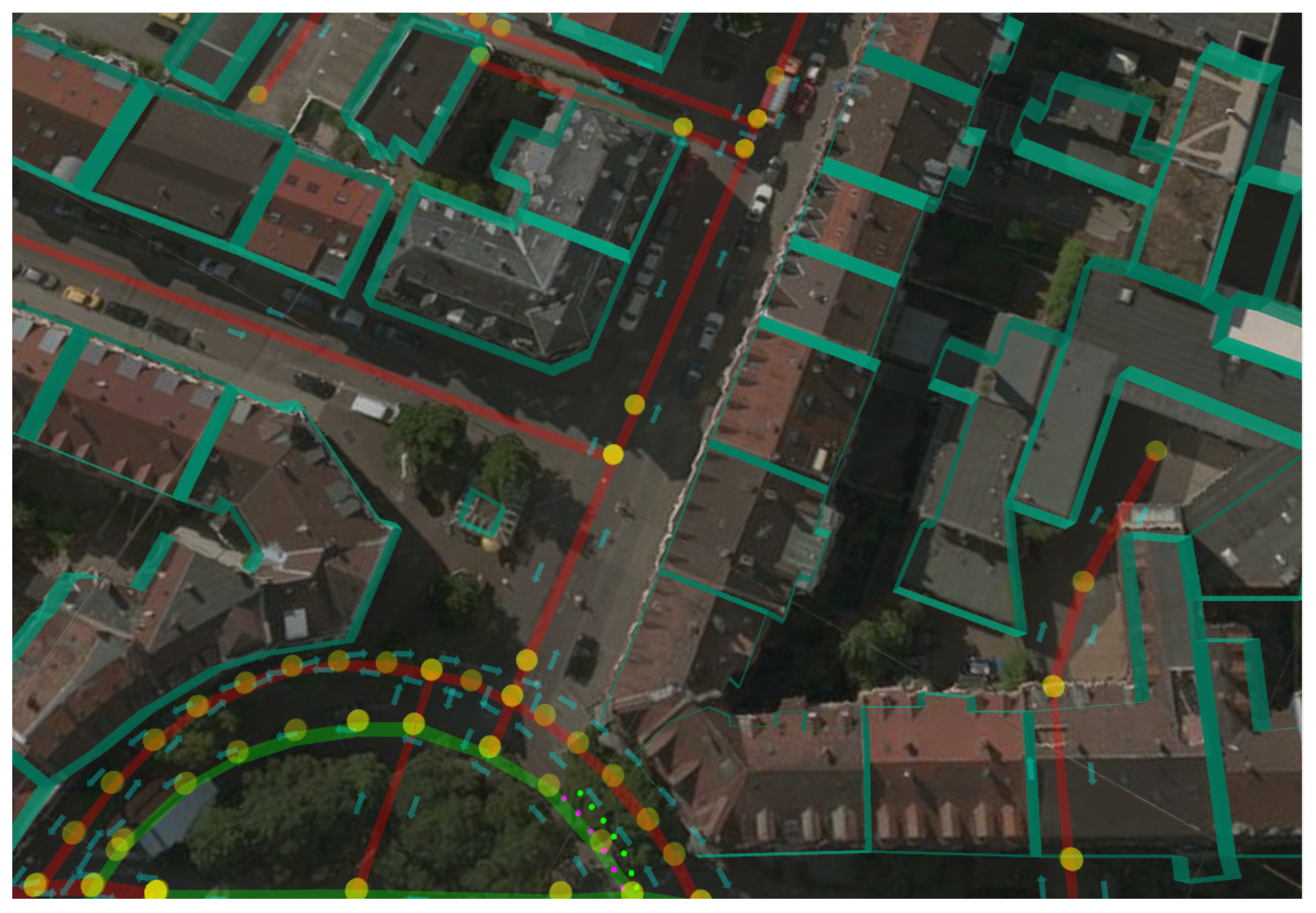
3. Proposed Localization Pipeline
3.1. Road Layout Estimation
- The Vehicle State, in terms of position, attitude, and speeds;
- The vector of LC, the scene elements associated with the hypothesis;
- The score of the layout, a value that combines the likelihoods of each of the LHs;
- The motion model to describe how the hypotheses evolve in time.
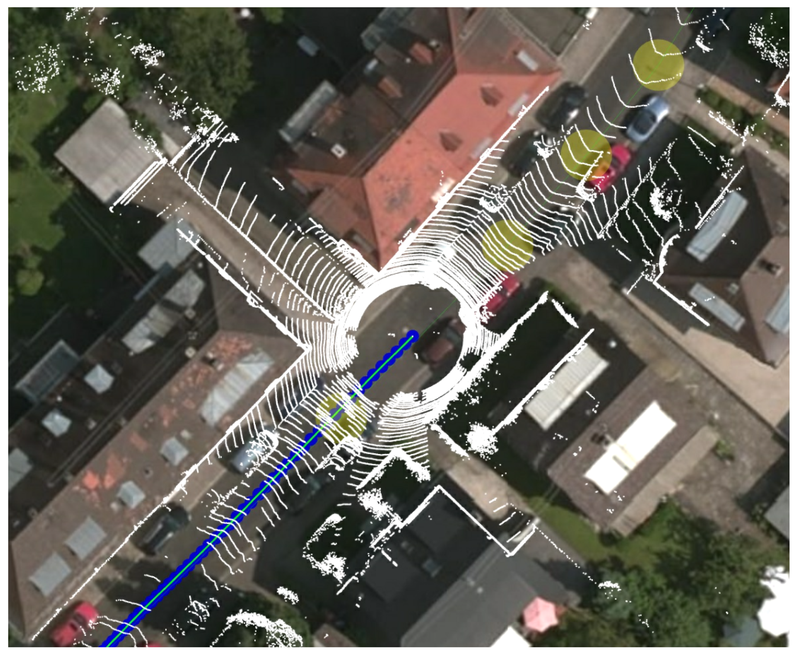
3.2. The Point Clouds
3.3. The Registration Step
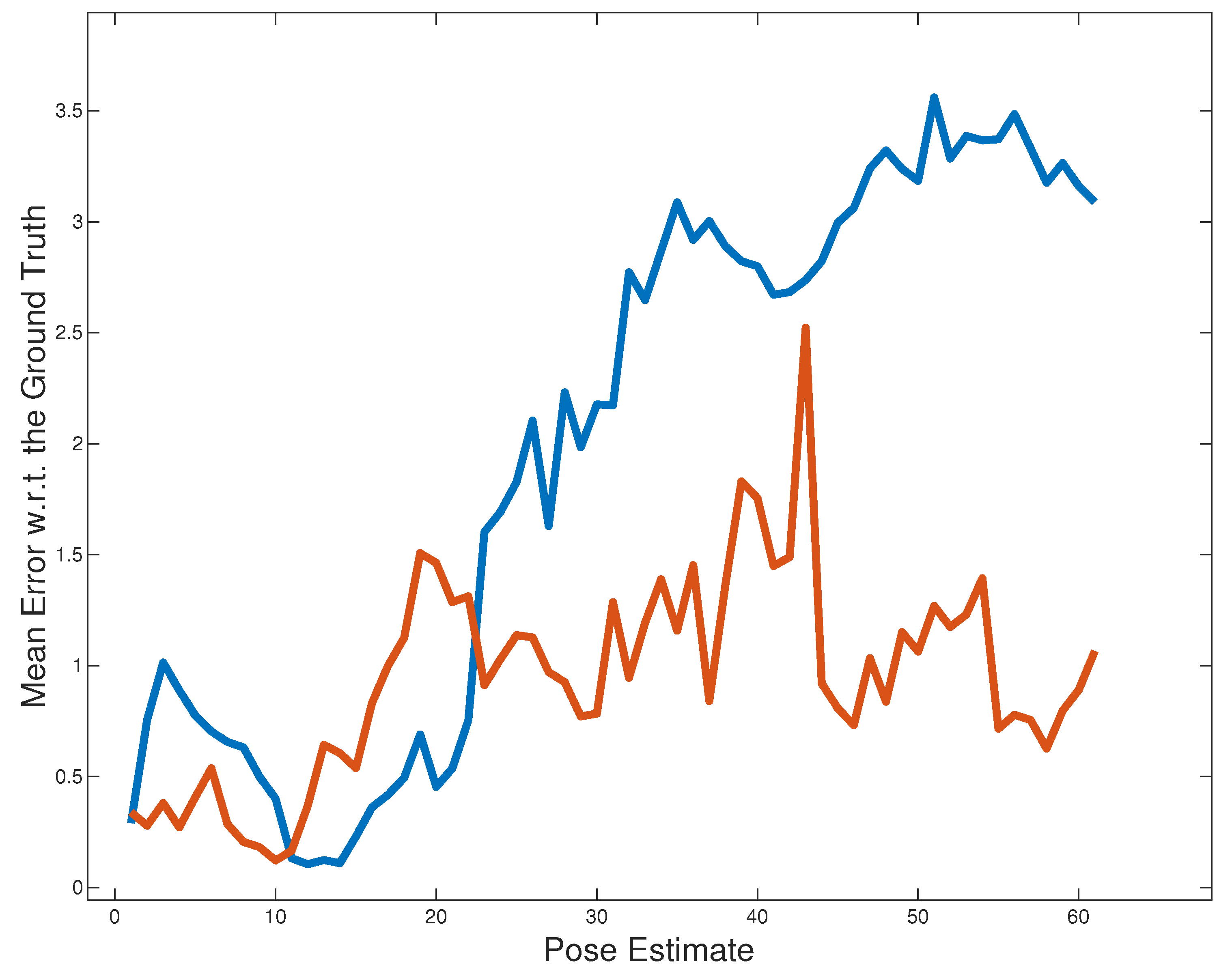
4. Experimental Results
5. Conclusions
Author Contributions
Funding
Institutional Review Board Statement
Informed Consent Statement
Data Availability Statement
Conflicts of Interest
Abbreviations
| RLE | Road Layout Estimation |
| CNN | Convolutional neural network |
| DNN | Deep neural network |
| GNSS | Global navigation satellite system |
| INS | Inertial navigation system |
| NLOS | Non-line-of-sight |
| LIDAR | Light detection and ranging |
| SGBM | Semi-global block matching |
| IoU | Intersection over union |
| ICP | Iterative closest point |
| OSM | OpenStreetMap |
| PC | Point Cloud |
| LC | Layout component |
| LH | Layout hypothesis |
| GT | Ground truth |
References
- Gu, Y.; Hsu, L.T.; Kamijo, S. GNSS/Onboard Inertial Sensor Integration With the Aid of 3-D Building Map for Lane-Level Vehicle Self-Localization in Urban Canyon. IEEE Trans. Veh. Technol. 2016, 65, 4274–4287. [Google Scholar] [CrossRef]
- Floros, G.; Leibe, B. Joint 2D-3D temporally consistent semantic segmentation of street scenes. In Proceedings of the 2012 IEEE Conference on Computer Vision and Pattern Recognition, Providence, RI, USA, 16–21 June 2012; pp. 2823–2830. [Google Scholar] [CrossRef]
- Fernández, C.; Izquierdo, R.; Llorca, D.F.; Sotelo, M.A. A Comparative Analysis of Decision Trees Based Classifiers for Road Detection in Urban Environments. In Proceedings of the 2015 IEEE 18th International Conference on Intelligent Transportation Systems, Gran Canaria, Spain, 15–18 September 2015; pp. 719–724. [Google Scholar] [CrossRef]
- Hummel, B.; Thiemann, W.; Lulcheva, I. Scene Understanding of Urban Road Intersections with Description Logic. In Logic and Probability for Scene Interpretation; Cohn, A.G., Hogg, D.C., Möller, R., Neumann, B., Eds.; Schloss Dagstuhl—Leibniz-Zentrum fuer Informatik, Germany: Dagstuhl, Germany, 2008. [Google Scholar]
- Corso, J.J. Discriminative modeling by Boosting on Multilevel Aggregates. In Proceedings of the 2008 IEEE Conference on Computer Vision and Pattern Recognition, Anchorage, AK, USA, 23–28 June 2008; pp. 1–8. [Google Scholar] [CrossRef]
- Hentschel, M.; Wagner, B. Autonomous robot navigation based on OpenStreetMap geodata. In Proceedings of the 13th International IEEE Conference on Intelligent Transportation Systems, Funchal, Portugal, 19–22 September 2010; pp. 1645–1650. [Google Scholar] [CrossRef]
- Larnaout, D.; Gay-Belllile, V.; Bourgeois, S.; Dhome, M. Vision-Based Differential GPS: Improving VSLAM/GPS Fusion in Urban Environment with 3D Building Models. IEEE Int. Conf. 3D Vis. (3DV) 2014, 1, 432–439. [Google Scholar] [CrossRef]
- Ruchti, P.; Steder, B.; Ruhnke, M.; Burgard, W. Localization on OpenStreetMap data using a 3D laser scanner. In Proceedings of the 2015 IEEE International Conference on Robotics and Automation (ICRA), Seattle, WA, USA, 26–30 May 2015; pp. 5260–5265. [Google Scholar] [CrossRef]
- Fernández, C.; Llorca, D.F.; Stiller, C.; Sotelo, M.A. Curvature-based curb detection method in urban environments using stereo and laser. In Proceedings of the 2015 IEEE Intelligent Vehicles Symposium (IV), Seoul, Korea, 28 June–1 July 2015; pp. 579–584. [Google Scholar] [CrossRef]
- Tao, Z.; Bonnifait, P.; Frémont, V.; Ibañez-Guzman, J.I. Mapping and localization using GPS, lane markings and proprioceptive sensors. In Proceedings of the 2013 IEEE/RSJ International Conference on Intelligent Robots and Systems, Tokyo, Japan, 3–7 November 2013; pp. 406–412. [Google Scholar] [CrossRef] [Green Version]
- Schreiber, M.; Knöppel, C.; Franke, U. LaneLoc: Lane marking based localization using highly accurate maps. In Proceedings of the 2013 IEEE Intelligent Vehicles Symposium (IV), Gold Coast, QLD, Australia, 23–26 June 2013; pp. 449–454. [Google Scholar] [CrossRef]
- Goodfellow, I.; Bengio, Y.; Courville, A. Deep Learning; The MIT Press: London, UK, 2016; Chapter 9. [Google Scholar]
- Ballardini, A.L.; Cattaneo, D.; Fontana, S.; Sorrenti, D.G. Leveraging the OSM building data to enhance the localization of an urban vehicle. In Proceedings of the 2016 IEEE 19th International Conference on Intelligent Transportation Systems (ITSC), Rio de Janeiro, Brazil, 1–4 November 2016; pp. 622–628. [Google Scholar] [CrossRef]
- Segal, A.; Haehnel, D.; Thrun, S. Generalized-icp. Robot. Sci. Syst. 2009, 2, 435. [Google Scholar]
- Geiger, A.; Lenz, P.; Stiller, C.; Urtasun, R. Vision meets Robotics: The KITTI Dataset. Int. J. Robot. Res. (IJRR) 2013, 32, 1231–1237. [Google Scholar] [CrossRef] [Green Version]
- Obradovic, D.; Lenz, H.; Schupfner, M. Fusion of Sensor Data in Siemens Car Navigation System. IEEE Trans. Veh. Technol. 2007, 56, 43–50. [Google Scholar] [CrossRef]
- Nedevschi, S.; Popescu, V.; Danescu, R.; Marita, T.; Oniga, F. Accurate Ego-Vehicle Global Localization at Intersections through Alignment of Visual Data with Digital Map. IEEE Trans. Intell. Transp. Syst. 2013, 14, 673–687. [Google Scholar] [CrossRef]
- Fairfield, N.; Urmson, C. Traffic light mapping and detection. In Proceedings of the 2011 IEEE International Conference on Robotics and Automation, Shanghai, China, 9–13 May 2011; pp. 5421–5426. [Google Scholar] [CrossRef] [Green Version]
- Raaijmakers, M.; Bouzouraa, M.E. In-vehicle Roundabout Perception Supported by a Priori Map Data. In Proceedings of the 2015 IEEE 18th International Conference on Intelligent Transportation Systems, Gran Canaria, Spain, 15–18 September 2015; pp. 437–443. [Google Scholar] [CrossRef]
- Ballardini, A.L.; Cattaneo, D.; Fontana, S.; Sorrenti, D.G. An online probabilistic road intersection detector. In Proceedings of the 2017 IEEE International Conference on Robotics and Automation (ICRA), Singapore, 29 May–3 June 2017; pp. 239–246. [Google Scholar] [CrossRef]
- Ballardini, A.L.; Cattaneo, D.; Sorrenti, D.G. Visual Localization at Intersections with Digital Maps. In Proceedings of the 2019 International Conference on Robotics and Automation (ICRA), Montreal, QC, Canada, 20–24 May 2019; pp. 6651–6657. [Google Scholar] [CrossRef]
- Ballardini, A.L.; Hernández, Á.; Ángel Sotelo, M. Model Guided Road Intersection Classification. arXiv 2021, arXiv:2104.12417. [Google Scholar]
- Ni, K.; Armstrong-Crews, N.; Sawyer, S. Geo-registering 3D point clouds to 2D maps with scan matching and the Hough Transform. In Proceedings of the 2013 IEEE International Conference on Acoustics, Speech and Signal Processing, Vancouver, BC, Canada, 26–31 May 2013; pp. 1864–1868. [Google Scholar] [CrossRef]
- Hsu, L.T. GNSS multipath detection using a machine learning approach. In Proceedings of the 2017 IEEE 20th International Conference on Intelligent Transportation Systems (ITSC), Yokohama, Japan, 16–19 October 2017; pp. 1–6. [Google Scholar] [CrossRef] [Green Version]
- Alonso, I.P.; Llorca, D.F.; Gavilan, M.; Pardo, S.A.; Garcia-Garrido, M.A.; Vlacic, L.; Sotelo, M.A. Accurate Global Localization Using Visual Odometry and Digital Maps on Urban Environments. IEEE Trans. Intell. Transp. Syst. 2012, 13, 1535–1545. [Google Scholar] [CrossRef] [Green Version]
- Floros, G.; van der Zander, B.; Leibe, B. OpenStreetSLAM: Global vehicle localization using OpenStreetMaps. In Proceedings of the 2013 IEEE International Conference on Robotics and Automation, Karlsruhe, Germany, 6–10 May 2013; pp. 1054–1059. [Google Scholar] [CrossRef]
- Xu, D.; Badino, H.; Huber, D. Topometric localization on a road network. In Proceedings of the 2014 IEEE/RSJ International Conference on Intelligent Robots and Systems, Chicago, IL, USA, 14–18 September 2014; pp. 3448–3455. [Google Scholar] [CrossRef] [Green Version]
- Ballardini, A.L.; Fontana, S.; Furlan, A.; Limongi, D.; Sorrenti, D.G. A Framework for Outdoor Urban Environment Estimation. In Proceedings of the 2015 IEEE 18th International Conference on Intelligent Transportation Systems, Gran Canaria, Spain, 15–18 September 2015; pp. 2721–2727. [Google Scholar] [CrossRef]
- David, P. Detecting Planar Surfaces in Outdoor Urban Environments; Technical Report ARL-TR-4599; United States Army Research Laboratory: Adelphi, MD, USA, 2008; Available online: https://apps.dtic.mil/sti/citations/ADA488059 (accessed on 5 August 2021).
- Delmerico, J.A.; David, P.; Corso, J.J. Building facade detection, segmentation, and parameter estimation for mobile robot localization and guidance. In Proceedings of the 2011 IEEE/RSJ International Conference on Intelligent Robots and Systems, San Francisco, CA, USA, 25–30 September 2011; pp. 1632–1639. [Google Scholar] [CrossRef] [Green Version]
- Baatz, G.; Köser, K.; Chen, D.; Grzeszczuk, R.; Pollefeys, M. Leveraging 3D City Models for Rotation Invariant Place-of-Interest Recognition. Int. J. Comp. Vis. 2012, 96, 315–334. [Google Scholar] [CrossRef]
- Musialski, P.; Wonka, P.; Aliaga, D.G.; Wimmer, M.; Gool, L.; Purgathofer, W. A Survey of Urban Reconstruction. J. Comp. Graph. Forum 2013, 32, 146–177. [Google Scholar] [CrossRef]
- Hirschmüller, H. Stereo processing by semiglobal matching and mutual information. IEEE Trans. Pattern Anal. Mach. Intell. 2008, 30, 328–341. [Google Scholar] [CrossRef]
- Scharstein, D.; Szeliski, R. A taxonomy and evaluation of dense two-frame stereo correspondence algorithms. Int. J. Comp. Vis. 2002, 47, 7–42. [Google Scholar] [CrossRef]
- Menze, M.; Heipke, C.; Geiger, A. Joint 3D estimation of vehicles and scene flow. ISPRS Ann. Photogramm. Remote Sens. Spat. Inf. Sci. 2015, II-3/W5, 427–434. [Google Scholar] [CrossRef] [Green Version]
- Poggi, M.; Kim, S.; Tosi, F.; Kim, S.; Aleotti, F.; Min, D.; Sohn, K.; Mattoccia, S. On the Confidence of Stereo Matching in a Deep-Learning Era: A Quantitative Evaluation. 2021. Available online: https://arxiv.org/abs/2101.00431 (accessed on 5 August 2021).
- Besl, P.J.; McKay, N.D. A method for registration of 3-D shapes. IEEE Trans. Pattern Anal. Mach. Intell. 1992, 14, 239–256. [Google Scholar] [CrossRef]
- Chen, Y.; Medioni, G. Object modelling by registration of multiple range images. Image Vis. Comp. 1992, 10, 145–155. [Google Scholar] [CrossRef]
- Pomerleau, F.; Colas, F.; Siegwart, R.; Magnenat, S. Comparing ICP variants on real-world data sets. Auton. Robot. 2013, 34, 133–148. [Google Scholar] [CrossRef]
- Fontana, S.; Cattaneo, D.; Ballardini, A.L.; Vaghi, M.; Sorrenti, D.G. A benchmark for point clouds registration algorithms. Robot. Auton. Syst. 2021, 140, 103734. [Google Scholar] [CrossRef]
- Agamennoni, G.; Fontana, S.; Siegwart, R.Y.; Sorrenti, D.G. Point clouds registration with probabilistic data association. In Proceedings of the 2016 IEEE/RSJ International Conference on Intelligent Robots and Systems (IROS), Daejeon, Korea, 9–14 October 2016; pp. 4092–4098. [Google Scholar]
- Rusu, R.B.; Blodow, N.; Marton, Z.C.; Beetz, M. Aligning point cloud views using persistent feature histograms. In Proceedings of the 2008 IEEE/RSJ International Conference on Intelligent Robots and Systems, Nice, France, 22–26 September 2008; pp. 3384–3391. [Google Scholar]
- Rusu, R.B.; Blodow, N.; Beetz, M. Fast point feature histograms (FPFH) for 3D registration. In Proceedings of the 2009 IEEE International Conference on Robotics and Automation, Kobe, Japan, 12–17 May 2009; pp. 3212–3217. [Google Scholar]
- Jiang, J.; Cheng, J.; Chen, X. Registration for 3-D point cloud using angular-invariant feature. Neurocomputing 2009, 72, 3839–3844. [Google Scholar] [CrossRef]
- Zeng, A.; Song, S.; Nießner, M.; Fisher, M.; Xiao, J.; Funkhouser, T. 3dmatch: Learning the matching of local 3d geometry in range scans. CVPR 2017, 1, 4. [Google Scholar]
- Gojcic, Z.; Zhou, C.; Wegner, J.D.; Wieser, A. The perfect match: 3D point cloud matching with smoothed densities. In Proceedings of the IEEE/CVF Conference on Computer Vision and Pattern Recognition, Long Beach, CA, USA, 15–20 June 2019; pp. 5545–5554. [Google Scholar]
- Aoki, Y.; Goforth, H.; Srivatsan, R.A.; Lucey, S. Pointnetlk: Robust & efficient point cloud registration using pointnet. In Proceedings of the IEEE/CVF Conference on Computer Vision and Pattern Recognition, Long Beach, CA, USA, 15–20 June 2019; pp. 7163–7172. [Google Scholar]
- Sarode, V.; Li, X.; Goforth, H.; Aoki, Y.; Srivatsan, R.A.; Lucey, S.; Choset, H. PCRNet: Point cloud registration network using PointNet encoding. arXiv 2019, arXiv:1908.07906. [Google Scholar]
- Zhou, Q.Y.; Park, J.; Koltun, V. Fast global registration. European Conference on Computer Vision. Available online: https://link.springer.com/chapter/10.1007/978-3-319-46475-6_47 (accessed on 5 August 2021).
- Yang, H.; Shi, J.; Carlone, L. Teaser: Fast and certifiable point cloud registration. IEEE Trans. Robot. 2020, 37, 314–333. [Google Scholar] [CrossRef]
- Dellaert, F.; Fox, D.; Burgard, W.; Thrun, S. Monte carlo localization for mobile robots. In Proceedings of the 1999 IEEE International Conference on Robotics and Automation (Cat. No. 99CH36288C), Detroit, MI, USA, 10–15 May 1999; Volume 2, pp. 1322–1328. [Google Scholar]
- Thrun, S.; Burgard, W.; Fox, D. Probabilistic Robotics (Intelligent Robotics and Autonomous Agents); The MIT Press: Cambridge, MA, USA, 2005; Chapter 4. [Google Scholar]
- Yu, F.; Koltun, V. Multi-Scale Context Aggregation by Dilated Convolutions. arXiv 2016, arXiv:1511.07122. [Google Scholar]
- Deng, J.; Dong, W.; Socher, R.; Li, L.J.; Li, K.; Fei-Fei, L. Imagenet: A large-scale hierarchical image database. In Proceedings of the 2009 IEEE Conference on Computer Vision and Pattern Recognition, Miami, FL, USA, 20–25 June 2009; pp. 248–255. [Google Scholar]
- Alhaija, H.A.; Mustikovela, S.K.; Mescheder, L.; Geiger, A.; Rother, C. Augmented Reality Meets Deep Learning for Car Instance Segmentation in Urban Scenes. Brit. Mach. Vis. Conf. (BMVC) 2017, 1, 2. [Google Scholar]
- Chang, J.R.; Chen, Y.S. Pyramid Stereo Matching Network. arXiv 2018, arXiv:1803.08669. [Google Scholar]
- Matthies, L.; Shafer, S. Error modeling in stereo navigation. IEEE J. Robot. Autom. 1987, 3, 239–248. [Google Scholar] [CrossRef] [Green Version]
- Mazzotti, C.; Sancisi, N.; Parenti-Castelli, V. A Measure of the Distance between Two Rigid-Body Poses Based on the Use of Platonic Solids. In ROMANSY 21—Robot Design, Dynamics and Control; Parenti-Castelli, V., Schiehlen, W., Eds.; Springer International Publishing: Cham, Switzerland, 2016; pp. 81–89. [Google Scholar]
- Holz, D.; Ichim, A.E.; Tombari, F.; Rusu, R.B.; Behnke, S. Registration with the point cloud library: A modular framework for aligning in 3-D. IEEE Robot. Autom. Mag. 2015, 22, 110–124. [Google Scholar] [CrossRef]


| Sequence | Duration [min:s] | Length [m] | Original Mean Error [m] | Proposal Mean Error [m] |
|---|---|---|---|---|
| 2011_09_26_drive_0005 | 0:16 | 66.10 | 2.043 | 0.941 |
| 2011_09_26_drive_0046 | 0:13 | 46.38 | 1.269 | 1.168 |
| 2011_09_26_drive_0095 | 0:27 | 252.63 | 1.265 | 0.963 |
| 2011_09_30_drive_0027 | 1:53 | 693.12 | 2.324 | 1.746 |
| 2011_09_30_drive_0028 | 7:02 | 3204.46 | 1.353 | 1.716 |
| Sequence | Duration [min:s] | Length [m] | Original Median Error [m] | Proposal Median Error [m] |
|---|---|---|---|---|
| 2011_09_26_drive_0005 | 0:16 | 66.10 | 2.307 | 0.925 |
| 2011_09_26_drive_0046 | 0:13 | 46.38 | 1.400 | 1.119 |
| 2011_09_26_drive_0095 | 0:27 | 252.63 | 1.237 | 0.902 |
| 2011_09_30_drive_0027 | 1:53 | 693.12 | 1.700 | 1.823 |
| 2011_09_30_drive_0028 | 7:02 | 3204.46 | 1.361 | 1.447 |
| Sequence | Duration [min:s] | Length [m] | Original Max Error [m] | Proposal Max Error [m] |
|---|---|---|---|---|
| 2011_09_26_drive_0005 | 0:16 | 66.10 | 3.560 | 2.522 |
| 2011_09_26_drive_0046 | 0:13 | 46.38 | 1.948 | 2.037 |
| 2011_09_26_drive_0095 | 0:27 | 252.63 | 3.166 | 2.694 |
| 2011_09_30_drive_0027 | 1:53 | 693.12 | 10.138 | 5.417 |
| 2011_09_30_drive_0028 | 7:02 | 3204.46 | 3.391 | 2.366 |
Publisher’s Note: MDPI stays neutral with regard to jurisdictional claims in published maps and institutional affiliations. |
© 2021 by the authors. Licensee MDPI, Basel, Switzerland. This article is an open access article distributed under the terms and conditions of the Creative Commons Attribution (CC BY) license (https://creativecommons.org/licenses/by/4.0/).
Share and Cite
Ballardini, A.L.; Fontana, S.; Cattaneo, D.; Matteucci, M.; Sorrenti, D.G. Vehicle Localization Using 3D Building Models and Point Cloud Matching. Sensors 2021, 21, 5356. https://doi.org/10.3390/s21165356
Ballardini AL, Fontana S, Cattaneo D, Matteucci M, Sorrenti DG. Vehicle Localization Using 3D Building Models and Point Cloud Matching. Sensors. 2021; 21(16):5356. https://doi.org/10.3390/s21165356
Chicago/Turabian StyleBallardini, Augusto Luis, Simone Fontana, Daniele Cattaneo, Matteo Matteucci, and Domenico Giorgio Sorrenti. 2021. "Vehicle Localization Using 3D Building Models and Point Cloud Matching" Sensors 21, no. 16: 5356. https://doi.org/10.3390/s21165356
APA StyleBallardini, A. L., Fontana, S., Cattaneo, D., Matteucci, M., & Sorrenti, D. G. (2021). Vehicle Localization Using 3D Building Models and Point Cloud Matching. Sensors, 21(16), 5356. https://doi.org/10.3390/s21165356