
Implementation of a Deep Learning Algorithm Based on Vertical Ground Reaction Force Time–Frequency Features for the Detection and Severity Classification of Parkinson’s Disease


Abstract
:1. Introduction
2. Materials and Methods
2.1. Gait in Parkinson’s Disease Database
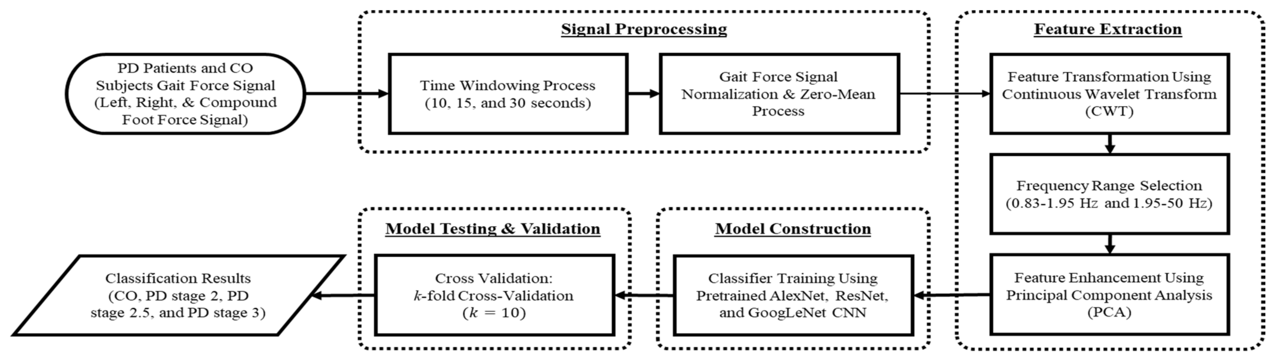
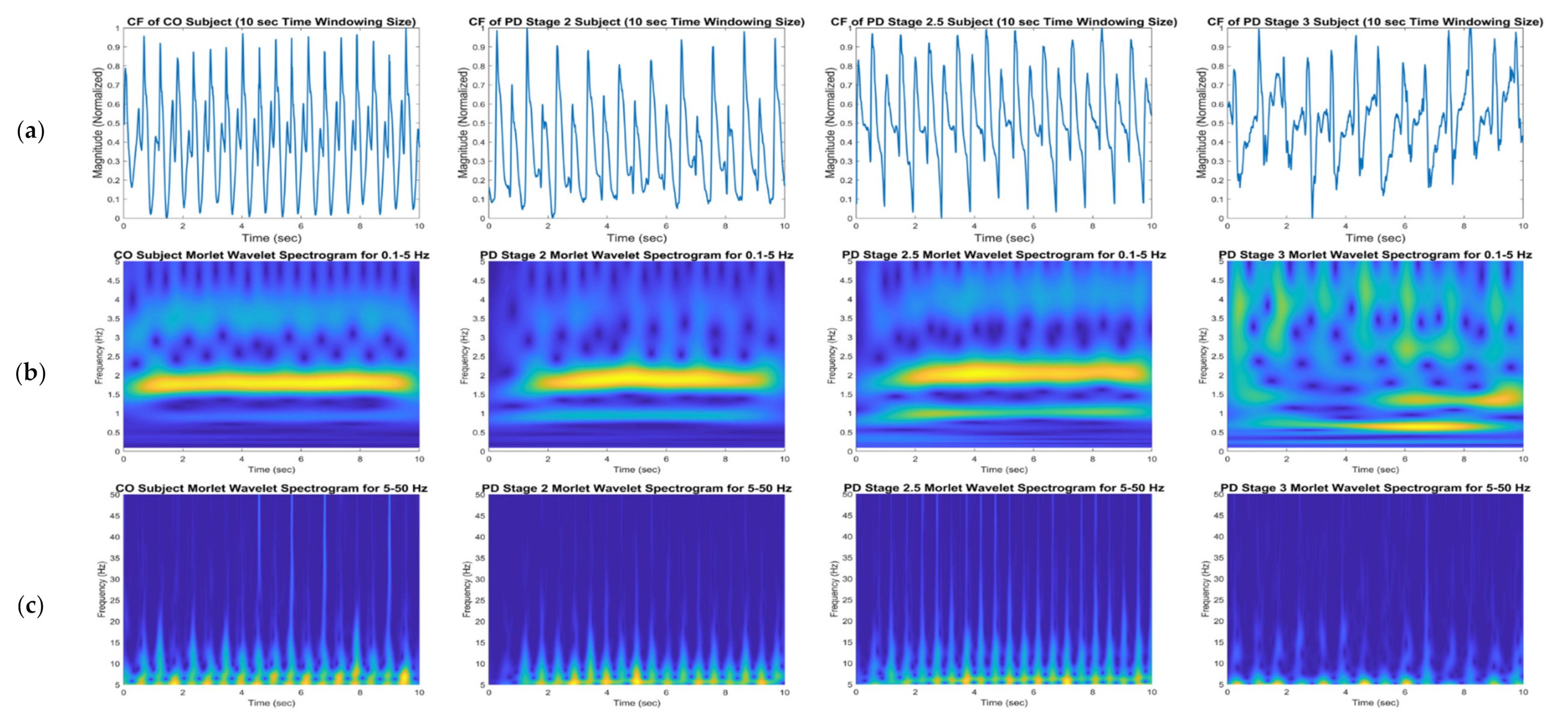
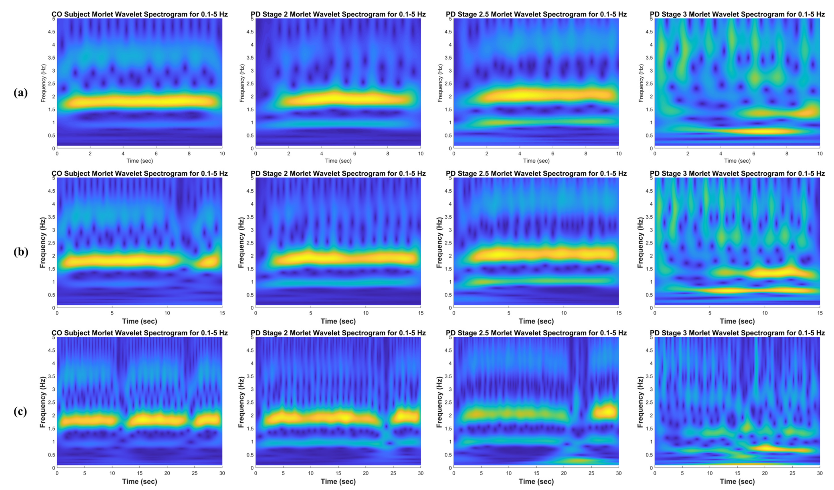
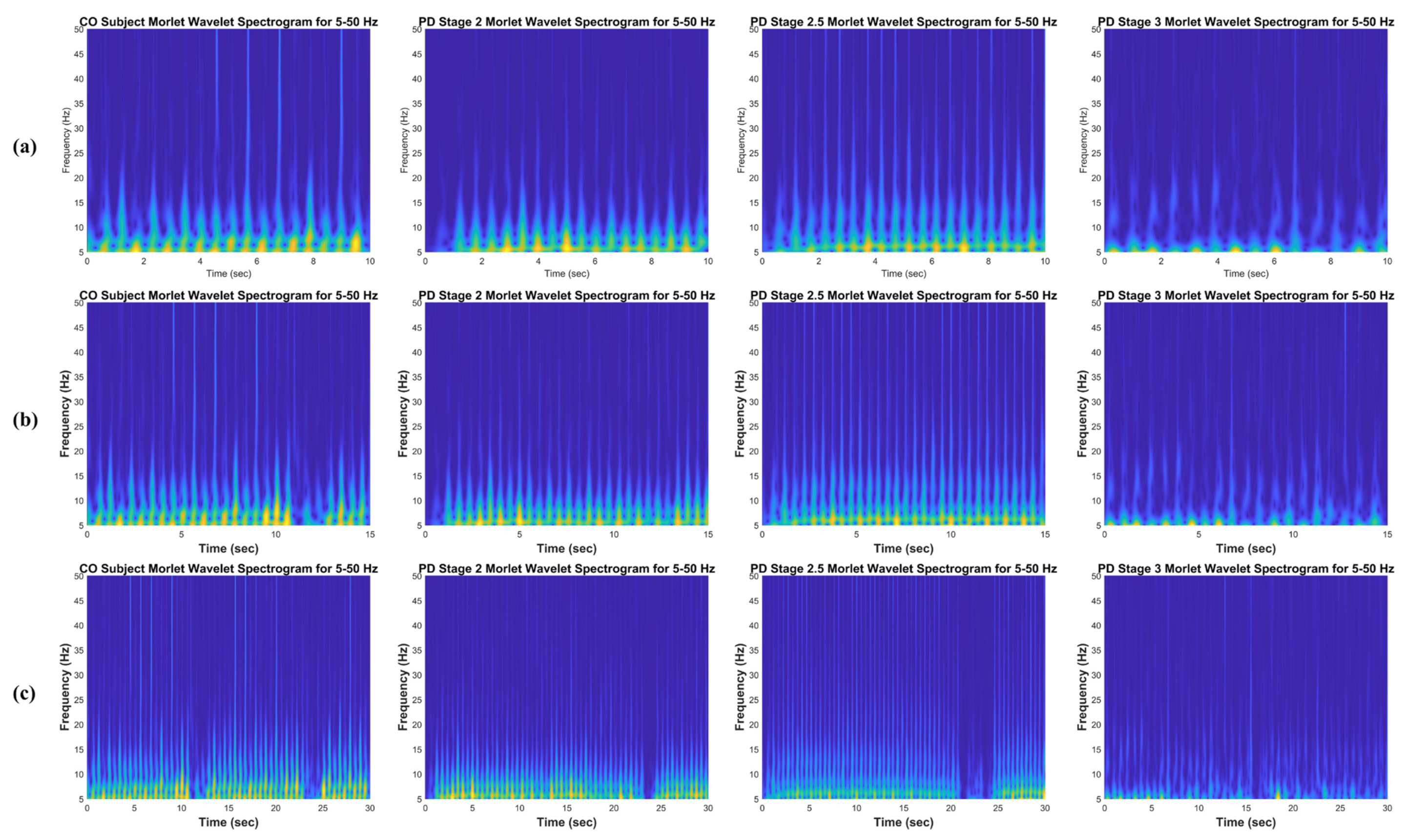
2.2. Signal Preprocessing
2.3. The Continuous Wavelet Transform
2.4. Principal Component Analysis
2.5. Convolutional Neural Network
2.5.1. AlexNet CNN
2.5.2. ResNet-50 and ResNet-101 CNN
2.5.3. GoogLeNet CNN
- An average pooling layer with a filter size and a stride of 3.
- A convolution with 128 filters for dimension reduction and rectified linear activation.
- A fully connected layer with 1024 units and rectified linear activation.
- A dropout layer with 70% rate of dropped outputs.
- A linear layer with softmax loss as the classifier.
2.6. Cross-Validation
3. Results
3.1. PD Severity Classification of Separated Ga, Ju, and Si Datasets
3.2. PD Severity Classification of All Datasets (Merged)
4. Discussion
4.1. Healthy Controls
4.2. Parkinson’s Disease Stage 2
4.3. Parkinson’s Disease Stage 2.5
4.4. Parkinson’s Disease Stage 3
4.5. Comparison of Results with the Existing Literature
5. Conclusions
Author Contributions
Funding
Institutional Review Board Statement
Informed Consent Statement
Data Availability Statement
Conflicts of Interest
References
- Lee, A.; Gilbert, R. Epidemiology of Parkinson Disease. Neurol. Clin. 2016, 34, 955–965. [Google Scholar] [CrossRef]
- Parkinson’s Disease Foundation. Statistics on Parkinson’s EIN: 13-1866796. 2018. Available online: https://bit.ly/2RCeh9H (accessed on 12 July 2019).
- National Institute of Neurological Disorders and Stroke. Parkinson’s Disease Information Page. 2016. Available online: https://bit.ly/2xTA6rL (accessed on 12 July 2019).
- Hoff, J.I.; Plas, A.A.; Wagemans, E.A.H.; Van Hilten, J.J. Accelerometric assessment of levodopa-induced dyskinesias in Parkinson’s disease. Mov. Disord. 2001, 16, 58–61. [Google Scholar] [CrossRef]
- Pistacchi, M.; Gioulis, M.; Sanson, F.; De Giovannini, E.; Filippi, G.; Rossetto, F.; Marsala, S.Z. Gait analysis and clinical correlations in early Parkinson’s disease. Funct Neurol. 2017, 32, 28. [Google Scholar] [CrossRef] [PubMed]
- Sofuwa, O.; Nieuwboer, A.; Desloovere, K.; Willems, A.-M.; Chavret, F.; Jonkers, I. Quantitative Gait Analysis in Parkinson’s Disease: Comparison with a Healthy Control Group. Arch. Phys. Med. Rehabil. 2005, 86, 1007–1013. [Google Scholar] [CrossRef] [Green Version]
- Lescano, C.N.; Rodrigo, S.E.; Christian, D.A. A possible parameter for gait clinimetric evaluation in Parkinson’s disease patients. J. Phys. Conf. Ser. 2016, 705, 12019. [Google Scholar] [CrossRef]
- Goldberger, A.L.; Amaral, L.A.; Glass, L.; Hausdorff, J.M.; Ivanov, P.C.; Mark, R.G.; Mietus, J.E.; Moody, G.B.; Peng, C.K.; Stanley, H.E. PhysioBank, PhysioToolkit, and PhysioNet: Components of a New Research Resource for Complex Physiologic Signals. Circulation 2003, 101, e215–e220. [Google Scholar] [CrossRef] [Green Version]
- Arafsha, F.; Hanna, C.; Aboualmagd, A.; Fraser, S.; El Saddik, A. Instrumented Wireless SmartInsole System for Mobile Gait Analysis: A Validation Pilot Study with Tekscan Strideway. J. Sens. Actuator Netw. 2018, 7, 36. [Google Scholar] [CrossRef] [Green Version]
- Hoehn, M.M.; Yahr, M.D. Parkinsonism: Onset, progression, and mortality. Neurology 1967, 17, 427. [Google Scholar] [CrossRef] [PubMed] [Green Version]
- Jane, Y.N.; Nehemiah, H.K.; Arputharaj, K. A Q-backpropagated time delay neural network for diagnosing severity of gait disturbances in Parkinson’s disease. J. Biomed. Inform. 2016, 60, 169–176. [Google Scholar] [CrossRef]
- Vasquez-Correa, J.C.; Arias-Vergara, T.; Orozco-Arroyave, J.R.; Eskofier, B.M.; Klucken, J.; Noth, E. Multimodal Assessment of Parkinson’s Disease: A Deep Learning Approach. IEEE J. Biomed. Health Inform. 2018, 23, 1618–1630. [Google Scholar] [CrossRef]
- Lee, S.-H.; Lim, J.S. Parkinson’s disease classification using gait characteristics and wavelet-based feature extraction. Expert Syst. Appl. 2012, 39, 7338–7344. [Google Scholar] [CrossRef]
- Zhao, A.; Qi, L.; Li, J.; Dong, J.; Yu, H. A hybrid spatio-temporal model for detection and severity rating of Parkinson’s disease from gait data. Neurocomputing 2018, 315, 1–8. [Google Scholar] [CrossRef] [Green Version]
- Hoffmann, A.G. General Limitations on Machine Learning. In Proceedings of the 9th European Conference on Artificial Intelligence, Stockholm, Sweden, 1 January 1990; pp. 345–347. [Google Scholar]
- Mastorakis, G. Human-like machine learning: Limitations and suggestions. arXiv 2018, arXiv:1811.06052. [Google Scholar]
- Jiang, X.; Napier, C.; Hannigan, B.; Eng, J.J.; Menon, C. Estimating Vertical Ground Reaction Force during Walking Using a Single Inertial Sensor. Sensors 2020, 20, 4345. [Google Scholar] [CrossRef]
- Lin, C.-W.; Wen, T.-C.; Setiawan, F. Evaluation of Vertical Ground Reaction Forces Pattern Visualization in Neurodegenerative Diseases Identification Using Deep Learning and Recurrence Plot Image Feature Extraction. Sensors 2020, 20, 3857. [Google Scholar] [CrossRef]
- Setiawan, F.; Lin, C.-W. Identification of Neurodegenerative Diseases Based on Vertical Ground Reaction Force Classification Using Time–Frequency Spectrogram and Deep Learning Neural Network Features. Brain Sci. 2021, 11, 902. [Google Scholar] [CrossRef]
- Alam, N.; Garg, A.; Munia, T.T.K.; Fazel-Rezai, R.; Tavakolian, K. Vertical ground reaction force marker for Parkinson’s disease. PLoS ONE 2017, 12, e0175951. [Google Scholar] [CrossRef]
- Yogev, G.; Giladi, N.; Peretz, C.; Springer, S.; Simon, E.S.; Hausdorff, J.M. Dual tasking, gait rhythmicity, and Parkinson’s disease: Which aspects of gait are attention demanding? Eur. J. Neurosci. 2005, 22, 1248–1256. [Google Scholar] [CrossRef]
- Hausdorff, J.M.; Lowenthal, J.; Herman, T.; Gruendlinger, L.; Peretz, C.; Giladi, N. Rhythmic auditory stimulation modulates gait variability in Parkinson’s disease. Eur. J. Neurosci. 2007, 26, 2369–2375. [Google Scholar] [CrossRef]
- Frenkel-Toledo, S.; Giladi, N.; Peretz, C.; Herman, T.; Gruendlinger, L.; Hausdorff, J.M. Treadmill walking as an external pacemaker to improve gait rhythm and stability in Parkinson’s disease. Mov. Disord. 2005, 20, 1109–1114. [Google Scholar] [CrossRef]
- Frenkel-Toledo, S.; Giladi, N.; Peretz, C.; Herman, T.; Gruendlinger, L.; Hausdorff, J.M. Effect of gait speed on gait rhythmicity in Parkinson’s disease: Variability of stride time and swing time respond differently. J. Neuroeng. Rehabil. 2005, 2, 23. [Google Scholar] [CrossRef] [Green Version]
- Fahn, S.; Marsden, C.D.; Calne, D.B.; Goldstein, M. Recent Developments in Parkinson’s Disease. Florham Park N. J. Macmillan Health Care Inf. 1987, 2, 153–164. [Google Scholar]
- Nilsson, J.; Thorstensson, A. Adaptability in frequency and amplitude of leg movements during human locomotion at different speeds. Acta Physiol. Scand. 1987, 129, 107–114. [Google Scholar] [CrossRef]
- Sadowsky, J. The continuous wavelet transform: A tool for signal investigation and understanding. Johns Hopkins APL Tech. Dig. 1994, 15, 306. [Google Scholar]
- Bernardino, A.; Santos-Victor, J. A real-time gabor primal sketch for visual attention. In Iberian Conference on Pattern Recognition and Image Analysis; Springer: Berlin/Heidelberg, Germany, 2005; pp. 335–342. [Google Scholar]
- Jolliffe, I.T. Introduction. In Principal Component Analysis, 2nd ed.; Springer: New York, NY, USA, 2002. [Google Scholar]
- O’Shea, K.; Nash, R. An introduction to convolutional neural networks. arXiv 2015, arXiv:1511.08458. [Google Scholar]
- Krizhevsky, A.; Sutskever, I.; Hinton, G.E. ImageNet classification with deep convolutional neural networks. Commun. ACM 2017, 60, 84–90. [Google Scholar] [CrossRef]
- He, K.; Zhang, X.; Ren, S.; Sun, J. Deep Residual Learning for Image Recognition. In Proceedings of the 2016 IEEE Conference on Computer Vision and Pattern Recognition (CVPR), Las Vegas, NV, USA, 27–30 June 2016; pp. 770–778. [Google Scholar] [CrossRef] [Green Version]
- Szegedy, C.; Liu, W.; Jia, Y.; Sermanet, P.; Reed, S.; Anguelov, D.; Erhan, D.; Vanhoucke, V.; Rabinovich, A. Going deeper with convolutions. In Proceedings of the 2015 IEEE Conference on Computer Vision and Pattern Recognition (CVPR), Boston, MA, USA, 7–12 June 2015; pp. 1–9. [Google Scholar] [CrossRef] [Green Version]
- Khan, A.; Sohail, A.; Zahoora, U.; Qureshi, A.S. A survey of the recent architectures of deep convolutional neural networks. Artif. Intell. Rev. 2020, 53, 5455–5516. [Google Scholar] [CrossRef] [Green Version]
- Alzubaidi, L.; Zhang, J.; Humaidi, A.J.; Al-Dujaili, A.; Duan, Y.; Al-Shamma, O.; Santamaría, J.; Fadhel, M.A.; Al-Amidie, M.; Farhan, L. Review of deep learning: Concepts, CNN architectures, challenges, applications, future directions. J. Big Data 2021, 8, 1–74. [Google Scholar] [CrossRef]
- Refaeilzadeh, P.; Tang, L.; Liu, H. Cross-Validation. Encycl. Database Syst. 2009, 532–538. [Google Scholar] [CrossRef]
- Fawcett, T. An introduction to ROC analysis. Pattern Recognit. Lett. 2006, 27, 861–874. [Google Scholar] [CrossRef]
- Youden, W.J. Index for rating diagnostic tests. Cancer 1950, 3, 32–35. [Google Scholar] [CrossRef]
- El Maachi, I.; Bilodeau, G.-A.; Bouachir, W. Deep 1D-Convnet for accurate Parkinson disease detection and severity prediction from gait. Expert Syst. Appl. 2020, 143, 113075. [Google Scholar] [CrossRef]
- Wu, Y.; Chen, P.; Luo, X.; Wu, M.; Liao, L.; Yang, S.; Rangayyan, R. Measuring signal fluctuations in gait rhythm time series of patients with Parkinson’s disease using entropy parameters. Biomed. Signal Process. Control. 2017, 31, 265–271. [Google Scholar] [CrossRef]
- Ertuğrul, Ö.F.; Kaya, Y.; Tekin, R.; Almali, M.N. Detection of Parkinson’s disease by Shifted One Dimensional Local Binary Patterns from gait. Expert Syst. Appl. 2016, 56, 156–163. [Google Scholar] [CrossRef]
- Zeng, W.; Liu, F.; Wang, Q.; Wang, Y.; Ma, L.; Zhang, Y. Parkinson’s disease classification using gait analysis via deterministic learning. Neurosci. Lett. 2016, 633, 268–278. [Google Scholar] [CrossRef] [PubMed]
- Daliri, M.R. Chi-square distance kernel of the gaits for the diagnosis of Parkinson’s disease. Biomed. Signal Process. Control. 2013, 8, 66–70. [Google Scholar] [CrossRef]
- Khoury, N.; Attal, F.; Amirat, Y.; Oukhellou, L.; Mohammed, S. Data-Driven Based Approach to Aid Parkinson’s Disease Diagnosis. Sensors 2019, 19, 242. [Google Scholar] [CrossRef] [Green Version]
- Khoury, N.; Attal, F.; Amirat, Y.; Chibani, A.; Mohammed, S. CDTW-Based Classification for Parkinson’s Disease Diagnosis. In Proceedings of the 26th European Symposium on Artificial Neural Networks, Bruges, Belgium, 25–27 April 2018. [Google Scholar]


| Stages | Description |
|---|---|
| 0 | No signs of disease |
| 1 | Symptoms are very mild; unilateral involvement only |
| 1.5 | Unilateral and axial involvement |
| 2 | Bilateral involvement without impairment of balance |
| 2.5 | Mild bilateral disease with recovery on pull test |
| 3 | Mild to moderate bilateral disease; some postural instability; physical independence |
| 4 | Severe disability; still able to walk or stand unassisted |
| 5 | Wheelchair bound or bedridden unless aided |
| Author | Stage 0 | Stage 2 | Stage 2.5 | Stage 3 |
|---|---|---|---|---|
| Ga [21] | 18 | 15 | 8 | 6 |
| Ju [22] | 26 | 12 | 13 | 4 |
| Si [23] | 29 | 29 | 6 | 0 |
| Layer Name | Output Size | 50 Layer | 101 Layer |
|---|---|---|---|
| conv1 | , , stride 2 | ||
| conv2_x | max pool, stride 2 | ||
| conv3_x | |||
| conv4_x | |||
| conv5_x | |||
| average pool, 1000-d fc, softmax | |||
| FLOPs | |||
| Architecture | Advantage | Disadvantage |
|---|---|---|
| AlexNet layer depth: 8 parameters: 60 million |
|
|
| ResNet-50 layer depth: 50 parameters: 25.6 million ResNet-101 layer depth: 101 parameters: 44.5 million |
|
|
| GoogLeNet layer depth: 22 parameters: 7 million |
|
|
| Time Window | Frequency Range | Disease Severity (Class) | AlexNet | ResNet-50 | ResNet-101 | GoogLeNet | ||||||||||||
|---|---|---|---|---|---|---|---|---|---|---|---|---|---|---|---|---|---|---|
| Sen (%) | Spec (%) | Acc (%) | AUC | Sen (%) | Spec (%) | Acc (%) | AUC | Sen (%) | Spec (%) | Acc (%) | AUC | Sen (%) | Spec (%) | Acc (%) | AUC | |||
| 10 s | 0.83–1.95 Hz | Class 0 | 98.21 | 98.11 | 98.14 | 0.9816 | 97.54 | 99.44 | 98.81 | 0.9849 | 97.54 | 99.56 | 98.89 | 0.9855 | 97.54 | 97.89 | 97.77 | 0.9771 |
| Class 2 | 93.29 | 97.78 | 96.14 | 0.9554 | 95.53 | 97.66 | 96.88 | 0.9659 | 97.15 | 96.49 | 96.73 | 0.9682 | 93.09 | 97.89 | 96.14 | 0.9549 | ||
| Class 2.5 | 82.50 | 96.12 | 93.69 | 0.8931 | 91.25 | 95.93 | 95.10 | 0.9359 | 88.75 | 97.29 | 95.77 | 0.9302 | 94.17 | 94.67 | 94.58 | 0.9442 | ||
| Class 3 | 83.93 | 97.37 | 95.69 | 0.9065 | 83.33 | 98.98 | 97.03 | 0.9116 | 88.10 | 99.32 | 97.92 | 0.9371 | 73.81 | 99.41 | 96.21 | 0.8661 | ||
| 1.95–50 Hz | Class 0 | 97.76 | 98.56 | 98.29 | 0.9816 | 95.30 | 98.89 | 97.70 | 0.9710 | 94.63 | 98.44 | 97.18 | 0.9654 | 97.09 | 97.78 | 97.55 | 0.9743 | |
| Class 2 | 95.93 * | 98.25 * | 97.40 * | 0.9709 * | 96.54 | 96.26 | 96.36 | 0.9640 | 96.34 | 94.74 | 95.32 | 0.9554 | 93.09 | 97.66 | 95.99 | 0.9538 | ||
| Class 2.5 | 93.75 * | 98.83 * | 97.92 * | 0.9629 * | 91.67 | 98.55 | 97.33 | 0.9511 | 87.50 | 98.01 | 96.14 | 0.9276 | 90.42 | 97.65 | 96.36 | 0.9403 | ||
| Class 3 | 96.43 | 99.15 | 98.81 | 0.9779 | 94.64 | 99.24 | 98.66 | 0.9694 | 89.29 | 99.24 | 98 | 0.9426 | 92.86 | 98.64 | 97.92 | 0.9575 | ||
| 15 s | 0.83–1.95 Hz | Class 0 | 97.98 | 98.33 | 98.22 | 0.9816 | 93.94 | 98.50 | 96.99 | 0.9622 | 95.29 | 99.33 | 97.99 | 0.9731 | 97.98 * | 99.17 * | 98.77 * | 0.9857 * |
| Class 2 | 94.21 | 96.66 | 95.76 | 0.9543 | 93.90 | 95.08 | 94.65 | 0.9449 | 97.26 | 95.43 | 96.10 | 0.9634 | 96.04 | 96.84 | 96.54 | 0.9644 | ||
| Class 2.5 | 85 | 97.29 | 95.09 | 0.9114 | 88.75 | 96.74 | 95.32 | 0.9275 | 90 | 98.51 | 96.99 | 0.9425 | 88.75 | 97.69 | 96.10 | 0.9322 | ||
| Class 3 | 90.18 | 98.60 | 97.55 | 0.9439 | 88.39 | 98.98 | 97.66 | 0.9369 | 95.54 | 99.62 | 99.11 | 0.9758 | 91.96 | 99.24 | 98.33 | 0.9560 | ||
| 1.95–50 Hz | Class 0 | 96.30 | 98.33 | 97.66 | 0.9731 | 93.94 | 98.50 | 96.99 | 0.9622 | 95.96 | 96.33 | 96.21 | 0.9615 | 95.96 | 98 | 97.32 | 0.9698 | |
| Class 2 | 93.29 | 97.54 | 95.99 | 0.9542 | 93.90 | 95.08 | 94.65 | 0.9449 | 91.77 | 95.78 | 94.31 | 0.9378 | 94.51 | 95.78 | 95.32 | 0.9515 | ||
| Class 2.5 | 88.13 | 97.56 | 95.88 | 0.9284 | 88.75 | 96.74 | 95.32 | 0.9275 | 89.38 | 96.47 | 95.21 | 0.9292 | 84.38 | 96.74 | 94.54 | 0.9056 | ||
| Class 3 | 94.64 | 97.96 | 97.55 | 0.9630 | 88.39 | 98.98 | 97.66 | 0.9369 | 81.25 | 99.36 | 97.10 | 0.9031 | 84.82 | 98.47 | 96.77 | 0.9165 | ||
| 30 s | 0.83–1.95 Hz | Class 0 | 95.24 | 98.33 | 97.32 | 0.9679 | 95.92 | 98.33 | 97.54 | 0.9713 | 91.84 | 99.67 | 97.09 | 0.9575 | 94.56 | 96.33 | 95.75 | 0.9545 |
| Class 2 | 93.90 | 97.17 | 95.97 | 0.9554 | 92.68 | 95.41 | 94.41 | 0.9404 | 95.73 | 91.87 | 93.29 | 0.9380 | 90.85 | 94.70 | 93.29 | 0.9278 | ||
| Class 2.5 | 95 | 97.55 | 97.09 | 0.9627 | 90 | 95.64 | 94.63 | 0.9282 | 85 | 94.82 | 93.06 | 0.8991 | 85 | 97.82 | 95.53 | 0.9141 | ||
| Class 3 | 94.64 | 99.49 | 98.88 | 0.9707 | 83.93 | 99.74 | 97.76 | 0.9184 | 76.79 | 99.74 | 96.87 | 0.8826 | 92.86 | 98.72 | 97.99 | 0.9579 | ||
| 1.95–50 Hz | Class 0 | 95.92 | 98 | 97.32 | 0.9696 | 93.20 | 99 | 97.09 | 0.9610 | 93.20 | 97.33 | 95.97 | 0.9527 | 95.24 | 97.33 | 96.64 | 0.9629 | |
| Class 2 | 93.29 | 95.76 | 94.85 | 0.9453 | 93.90 | 94.35 | 94.18 | 0.9412 | 93.30 | 92.58 | 93.06 | 0.9324 | 88.41 | 94.35 | 92.17 | 0.9138 | ||
| Class 2.5 | 80 | 98.37 | 95.08 | 0.8918 | 86.25 | 94.82 | 93.29 | 0.9054 | 82.50 | 95.91 | 93.51 | 0.8921 | 76.25 | 94.28 | 91.05 | 0.8526 | ||
| Class 3 | 98.21 * | 97.44 * | 97.54 * | 0.9783 * | 80.36 | 98.98 | 96.64 | 0.8967 | 76.79 | 99.23 | 96.42 | 0.8801 | 83.93 | 97.70 | 95.97 | 0.9081 | ||
| Time Window | Frequency Range | Disease Severity (Class) | AlexNet | ResNet-50 | ResNet-101 | GoogLeNet | ||||||||||||
|---|---|---|---|---|---|---|---|---|---|---|---|---|---|---|---|---|---|---|
| Sen (%) | Spec (%) | Acc (%) | AUC | Sen (%) | Spec (%) | Acc (%) | AUC | Sen (%) | Spec (%) | Acc (%) | AUC | Sen (%) | Spec (%) | Acc (%) | AUC | |||
| 10 s | 0.83–1.95 Hz | Class 0 | 94.47 | 99.02 | 98.21 | 0.9675 | 96.98 * | 99.67 * | 99.20 * | 0.9833 * | 93.97 | 99.02 | 98.13 | 0.9650 | 97.49 | 98.48 | 98.30 | 0.9798 |
| Class 2 | 93.75 | 98.05 | 96.70 | 0.9590 | 96.59 * | 98.44 * | 97.86 * | 0.9751 * | 95.17 | 94.66 | 94.82 | 0.9492 | 93.75 | 95.96 | 95.27 | 0.9486 | ||
| Class 2.5 | 94.13 | 94.85 | 94.55 | 0.9449 | 98.26 | 93.64 | 95.54 | 0.9595 | 92.61 | 95.61 | 94.38 | 0.9411 | 93.26 | 94.09 | 93.75 | 0.9368 | ||
| Class 3 | 80.73 | 97.73 | 96.07 | 0.8923 | 70.64 | 99.90 | 97.05 | 0.8527 | 80.73 | 99.51 | 97.68 | 0.9012 | 71.56 | 99.51 | 96.79 | 0.8553 | ||
| 1.95–50 Hz | Class 0 | 96.48 | 98.70 | 98.30 | 0.9759 | 94.47 | 99.46 | 98.57 | 0.9696 | 94.97 | 98.91 | 98.21 | 0.9694 | 92.46 | 98.70 | 97.59 | 0.9558 | |
| Class 2 | 92.90 | 98.70 | 96.88 | 0.9580 | 93.18 | 97.01 | 95.80 | 0.9509 | 95.45 | 94.79 | 95 | 0.9512 | 93.47 | 96.35 | 95.45 | 0.9491 | ||
| Class 2.5 | 97.39 * | 96.52 * | 96.88 * | 0.9695 * | 96.52 | 95.45 | 95.89 | 0.9599 | 92.83 | 96.97 | 95.27 | 0.9490 | 93.70 | 97.12 | 95.71 | 0.9541 | ||
| Class 3 | 90.83 | 99.11 | 98.30 | 0.9497 | 89.91 | 99.60 | 98.66 | 0.9476 | 87.16 | 99.70 | 98.48 | 0.9343 | 93.58 | 98.52 | 98.04 | 0.9605 | ||
| 15 s | 0.83–1.95 Hz | Class 0 | 93.80 | 99.17 | 98.22 | 0.9648 | 96.12 | 98.84 | 98.36 | 0.9748 | 93.80 | 98.67 | 97.81 | 0.9623 | 93.02 | 99.50 | 98.36 | 0.9626 |
| Class 2 | 95.63 | 97.60 | 96.99 | 0.9662 | 91.27 | 98 | 95.89 | 0.9464 | 92.14 | 97.41 | 95.75 | 0.9477 | 96.51 | 95.81 | 96.03 | 0.9616 | ||
| Class 2.5 | 94.33 | 96.98 | 95.89 | 0.9566 | 96.67 | 95.35 | 95,89 | 0.9601 | 96.67 | 94.88 | 95.62 | 0.9578 | 92 | 97.21 | 95.07 | 0.9460 | ||
| Class 3 | 88.89 | 98.02 | 97.12 | 0.9346 | 90.28 | 99.24 | 98.36 | 0.9476 | 83.33 | 99.24 | 97.67 | 0.9129 | 90.28 | 98.18 | 97.40 | 0.9423 | ||
| 1.95–50 Hz | Class 0 | 90.70 | 98.50 | 97.12 | 0.9460 | 87.60 | 99.17 | 97.12 | 0.9338 | 93.80 | 98.17 | 97.40 | 0.9598 | 89.92 | 98 | 96.58 | 0.9396 | |
| Class 2 | 93.01 | 97.01 | 95.75 | 0.9501 | 93.89 | 96.01 | 95.34 | 0.9495 | 93.45 | 94.61 | 94.25 | 0.9403 | 88.21 | 96.41 | 93.84 | 0.9231 | ||
| Class 2.5 | 94.67 | 97.44 | 96.30 | 0.9605 | 94.33 | 96.05 | 95.34 | 0.9519 | 91.67 | 95.58 | 93.97 | 0.9362 | 94.67 | 93.95 | 94.25 | 0.9431 | ||
| Class 3 | 94.44 | 98.02 | 97.67 | 0.9623 | 88.89 | 98.02 | 97.12 | 0.9346 | 79.17 | 99.09 | 97.12 | 0.8913 | 86.11 | 98.48 | 97.26 | 0.9230 | ||
| 30 s | 0.83–1.95 Hz | Class 0 | 86.21 | 98.52 | 96.37 | 0.9237 | 91.38 | 100 | 98.49 | 0.9569 | 89.66 | 100 | 98.19 | 0.9483 | 84.48 | 98.17 | 95.77 | 0.9133 |
| Class 2 | 92.23 | 93.86 | 93.35 | 0.9305 | 96.12 | 96.49 | 96.37 | 0.9630 | 96.12 | 95.61 | 95.77 | 0.9587 | 85.44 | 94.74 | 91.84 | 0.9009 | ||
| Class 2.5 | 91.85 | 96.94 | 94.86 | 0.9440 | 96.30 | 93.88 | 94.86 | 0.9509 | 96.30 | 89.29 | 92.15 | 0.9279 | 96.30 | 92.35 | 93.96 | 0.9432 | ||
| Class 3 | 97.14 * | 98.65 * | 98.49 * | 0.9790 * | 77.14 | 99.32 | 96.98 | 0.8823 | 51.43 | 99.66 | 94.56 | 0.7555 | 85.71 | 99.32 | 97.89 | 0.9252 | ||
| 1.95–50 Hz | Class 0 | 89.66 | 97.07 | 95.77 | 0.9336 | 79.31 | 100 | 96.37 | 0.8966 | 81.03 | 98.53 | 95.47 | 0.8978 | 82.76 | 94.87 | 92.75 | 0.8882 | |
| Class 2 | 83.50 | 96.05 | 92.15 | 0.8977 | 85.44 | 93.42 | 90.94 | 0.8943 | 90.29 | 90.79 | 90.63 | 0.9054 | 79.61 | 92.98 | 88.82 | 0.8630 | ||
| Class 2.5 | 93.33 | 93.37 | 93.35 | 0.9335 | 95.56 | 87.24 | 90.63 | 0.9140 | 91.11 | 87.76 | 89.12 | 0.8943 | 89.63 | 93.37 | 91.84 | 0.9150 | ||
| Class 3 | 91.43 | 98.31 | 97.58 | 0.9487 | 71.43 | 98.89 | 96.07 | 0.8521 | 48.57 | 99.32 | 93.96 | 0.7395 | 82.86 | 97.30 | 95.77 | 0.9008 | ||
| Time Window | Frequency Range | Disease Severity (Class) | AlexNet | ResNet-50 | ResNet-101 | GoogLeNet | ||||||||||||
|---|---|---|---|---|---|---|---|---|---|---|---|---|---|---|---|---|---|---|
| Sen (%) | Spec (%) | Acc (%) | AUC | Sen (%) | Spec (%) | Acc (%) | AUC | Sen (%) | Spec (%) | Acc (%) | AUC | Sen (%) | Spec (%) | Acc (%) | AUC | |||
| 10 s | 0.83–1.95 Hz | Class 0 | 97.99 | 98.10 | 98.05 | 0.9804 | 97.70 | 99.52 | 98.70 | 0.9861 | 97.99 | 97.38 | 97.66 | 0.9768 | 97.13 | 96.67 | 96.88 | 0.9690 |
| Class 2 | 94.64 | 91.20 | 92.71 | 0.9292 | 97.92 | 95.60 | 96.61 | 0.9676 | 95.83 | 94.91 | 95.31 | 0.9537 | 94.35 | 92.82 | 93.49 | 0.9358 | ||
| Class 2.5 | 61.90 | 98.39 | 94.40 | 0.8015 | 86.90 | 99.27 | 97.92 | 0.9309 | 82.14 | 99.56 | 97.66 | 0.9085 | 73.81 | 99.12 | 96.35 | 0.8647 | ||
| 1.95–50 Hz | Class 0 | 98.56 * | 99.05 * | 98.83 * | 0.9881 * | 96.84 | 99.05 | 98.05 | 0.9794 | 96.26 | 96.43 | 96.35 | 0.9635 | 95.98 | 98.57 | 97.40 | 0.9727 | |
| Class 2 | 95.83 * | 98.84 * | 97.53 * | 0.9734 * | 97.32 | 96.06 | 96.61 | 0.9669 | 95.54 | 93.52 | 94.40 | 0.9453 | 94.64 | 93.98 | 94.27 | 0.9431 | ||
| Class 2.5 | 98.81 * | 98.39 * | 98.44 * | 0.9860 * | 91.67 | 99.12 | 98.31 | 0.9539 | 80.95 | 99.85 | 97.79 | 0.9040 | 84.52 | 98.10 | 96.61 | 0.9131 | ||
| 15 s | 0.83–1.95 Hz | Class 0 | 97.41 | 97.50 | 97.46 | 0.9746 | 96.12 | 99.29 | 97.85 | 0.9770 | 96.55 | 97.86 | 97.27 | 0.9720 | 99.14 | 97.14 | 98.05 | 0.9814 |
| Class 2 | 92.41 | 94.79 | 93.75 | 0.9360 | 96.88 | 94.10 | 95.31 | 0.9549 | 95.98 | 95.14 | 95.51 | 0.9556 | 93.30 | 97.57 | 95.70 | 0.9544 | ||
| Class 2.5 | 82.14 | 97.59 | 95.90 | 0.8987 | 85.71 | 98.90 | 97.46 | 0.9231 | 87.50 | 99.12 | 97.85 | 0.9331 | 91.07 | 98.46 | 97.66 | 0.9477 | ||
| 1.95–50 Hz | Class 0 | 94.83 | 98.57 | 96.88 | 0.9670 | 93.53 | 98.57 | 96.29 | 0.9605 | 96.12 | 97.50 | 96.88 | 0.9681 | 96.12 | 96.79 | 96.48 | 0.9645 | |
| Class 2 | 93.30 | 95.49 | 94.53 | 0.9439 | 96.43 | 92.36 | 94.14 | 0.9439 | 95.09 | 93.40 | 94.14 | 0.9425 | 95.54 | 94.44 | 94.92 | 0.9499 | ||
| Class 2.5 | 96.43 | 97.37 | 97.27 | 0.9690 | 85.71 | 98.90 | 97.46 | 0.9231 | 80.36 | 98.90 | 96.88 | 0.8963 | 85.71 | 99.56 | 98.05 | 0.9264 | ||
| 30 s | 0.83–1.95 Hz | Class 0 | 93.97 | 96.43 | 95.31 | 0.9520 | 93.97 | 97.86 | 96.09 | 0.9591 | 94.83 | 96.43 | 95.70 | 0.9563 | 95.69 | 97.86 | 96.88 | 96.77 |
| Class 2 | 92.86 | 93.75 | 93.36 | 0.9330 | 94.64 | 93.75 | 94.14 | 0.9420 | 95.54 | 88.19 | 91.41 | 0.9187 | 92.86 | 93.75 | 93.36 | 93.30 | ||
| Class 2.5 | 89.29 | 98.25 | 97.27 | 0.9377 | 89.29 | 98.25 | 97.27 | 0.9377 | 57.14 | 99.56 | 94.92 | 0.7835 | 82.14 | 97.37 | 95.70 | 89.76 | ||
| 1.95–50 Hz | Class 0 | 97.41 | 94.29 | 95.70 | 0.9585 | 93.10 | 98.57 | 96.09 | 0.9584 | 94.83 | 95 | 94.92 | 0.9491 | 93.10 | 98.57 | 96.09 | 0.9584 | |
| Class 2 | 88.39 | 93.75 | 91.41 | 0.9107 | 93.75 | 89.58 | 91.41 | 0.9167 | 90.18 | 89.58 | 89.84 | 89.88 | 91.07 | 93.06 | 92.19 | 0.9206 | ||
| Class 2.5 | 75 | 97.37 | 94.92 | 0.8618 | 71.43 | 97.37 | 94.53 | 0.8440 | 64.29 | 97.81 | 94.14 | 81.05 | 92.86 | 96.49 | 96.09 | 0.9467 | ||
| Time Window | Frequency Range | Disease Severity (Class) | AlexNet | ResNet-50 | ResNet-101 | GoogLeNet | ||||||||||||
|---|---|---|---|---|---|---|---|---|---|---|---|---|---|---|---|---|---|---|
| Sen (%) | Spec (%) | Acc (%) | AUC | Sen (%) | Spec (%) | Acc (%) | AUC | Sen (%) | Spec (%) | Acc (%) | AUC | Sen (%) | Spec (%) | Acc (%) | AUC | |||
| 10 s | 0.83–1.95 Hz | Class 0 | 98.88 | 98.11 | 98.37 | 0.9850 | 97.76 | 99.11 | 98.66 | 0.9844 | 98.43 * | 99 * | 98.81 * | 0.9872 * | 96.20 | 98.89 | 98 | 0.9754 |
| Class 2 | 95.33 | 95.56 | 95.47 | 0.9544 | 94.92 | 97.54 | 96.59 | 0.9623 | 95.53 | 97.19 | 96.59 | 0.9636 | 93.50 | 96.61 | 95.47 | 0.9505 | ||
| Class 2.5 | 76.25 | 96.21 | 92.65 | 0.8623 | 91.67 | 97.02 | 96.07 | 0.9434 | 89.58 | 95.93 | 94.80 | 0.9276 | 89.17 | 94.94 | 93.91 | 0.9205 | ||
| Class 3 | 78.57 | 97.96 | 95.55 | 0.8827 | 90.48 | 99.24 | 98.14 | 0.9486 | 80.95 | 99.32 | 97.03 | 0.9014 | 79.76 | 98.81 | 96.44 | 0.8929 | ||
| 1.95–50 Hz | Class 0 | 97.76 | 99.67 | 99.03 | 0.9871 | 94.85 | 98.89 | 97.55 | 0.9687 | 96.20 | 97.78 | 97.25 | 0.9699 | 96.42 | 97.56 | 97.18 | 0.9699 | |
| Class 2 | 97.97 * | 97.78 * | 97.85 * | 0.9787 * | 96.14 | 96.02 | 96.07 | 0.9608 | 94.31 | 96.26 | 95.55 | 0.9528 | 90.04 | 96.96 | 94.43 | 0.9350 | ||
| Class 2.5 | 89.17 | 98.28 | 96.66 | 0.9373 | 91.67 | 98.28 | 97.10 | 0.9498 | 90 | 97.29 | 95.99 | 0.9364 | 86.67 | 94.85 | 93.39 | 0.9076 | ||
| Class 3 | 93.45 | 98.64 | 98 | 0.9605 | 94.05 * | 99.24 * | 98.59 * | 0.9664 * | 86.90 | 99.24 | 97.70 | 0.9307 | 82.14 | 98.13 | 96.14 | 0.9014 | ||
| 15 s | 0.83–1.95 Hz | Class 0 | 97.31 | 99 | 98.44 | 0.9815 | 96.63 | 99.50 | 98.55 | 0.9807 | 95.96 | 99 | 97.99 | 0.9748 | 98.98 | 98.17 | 98.10 | 0.9807 |
| Class 2 | 93.90 | 98.24 | 96.66 | 0.9607 | 96.95 | 97.01 | 96.99 | 0.9698 | 96.04 | 96.13 | 96.10 | 0.9609 | 90.85 | 96.66 | 94.54 | 0.9376 | ||
| Class 2.5 | 96.88 * | 96.88 * | 96.88 * | 0.9688 * | 92.50 | 97.83 | 96.88 | 0.9516 | 92.50 | 97.15 | 96.32 | 0.9483 | 87.50 | 95.79 | 94.31 | 0.9165 | ||
| Class 3 | 91.96 | 99.82 | 98.66 | 0.9579 | 92.86 | 99.49 | 98.66 | 0.9617 | 88.39 | 99.87 | 98.44 | 0.9413 | 89.29 | 99.11 | 97.88 | 0.9420 | ||
| 1.95–50 Hz | Class 0 | 98.32 | 98.33 | 98.33 | 0.9832 | 95.29 | 98.50 | 97.44 | 0.9689 | 93.94 | 98.67 | 97.10 | 0.9630 | 95.96 | 97.33 | 96.88 | 0.9665 | |
| Class 2 | 94.21 | 98.77 | 97.10 | 0.9649 | 92.38 | 97.01 | 95.32 | 0.9470 | 95.43 | 93.67 | 94.31 | 0.9455 | 91.16 | 94.73 | 93.42 | 0.9294 | ||
| Class 2.5 | 87.50 | 97.96 | 96.10 | 0.9273 | 90.63 | 96.61 | 95.54 | 0.9362 | 83.75 | 95.93 | 93.76 | 0.8984 | 78.13 | 97.56 | 94.09 | 0.8784 | ||
| Class 3 | 94.64 | 97.71 | 97.32 | 0.9617 | 91.96 | 98.47 | 97.66 | 0.9522 | 79.46 | 98.98 | 96.54 | 0.8922 | 95.54 | 97.83 | 97.55 | 0.9669 | ||
| 30 s | 0.83–1.95 Hz | Class 0 | 96.60 | 98.67 | 97.99 | 0.9763 | 95.24 | 99.67 | 98.21 | 0.9745 | 94.56 | 99.33 | 97.76 | 0.9695 | 93.20 | 98.33 | 96.64 | 0.9577 |
| Class 2 | 96.34 | 96.47 | 96.42 | 0.9640 | 96.34 | 97.17 | 96.87 | 0.9676 | 96.34 | 92.58 | 93.96 | 0.9446 | 95.73 | 92.23 | 93.51 | 0.9398 | ||
| Class 2.5 | 88.75 | 98.37 | 96.64 | 0.9356 | 96.25 | 97 | 96.87 | 0.9663 | 81.25 | 94.28 | 91.95 | 0.8776 | 77.50 | 97.28 | 93.74 | 0.8739 | ||
| Class 3 | 92.86 | 98.98 | 98.21 | 0.9592 | 89.29 | 99.49 | 98.21 | 0.9439 | 69.64 | 99.49 | 95.75 | 0.8457 | 85.71 | 98.47 | 96.87 | 0.9209 | ||
| 1.95–50 Hz | Class 0 | 93.20 | 97.33 | 95.97 | 0.9527 | 91.84 | 97.67 | 95.75 | 0.9475 | 93.88 | 97.67 | 96.42 | 0.9577 | 93.88 | 96.33 | 95.53 | 0.9511 | |
| Class 2 | 92.07 | 94.35 | 93.51 | 0.9321 | 88.41 | 94.35 | 92.17 | 0.9138 | 91.46 | 92.23 | 91.95 | 0.9184 | 85.98 | 93.29 | 90.60 | 0.8963 | ||
| Class 2.5 | 80 | 97.55 | 94.41 | 0.8877 | 90 | 94.01 | 93.29 | 0.9200 | 81.25 | 92.64 | 90.60 | 0.8695 | 73.75 | 94.01 | 90.38 | 0.8388 | ||
| Class 3 | 92.86 | 97.44 | 96.87 | 0.9515 | 82.14 | 98.98 | 96.87 | 0.9056 | 64.29 | 99.49 | 95.08 | 0.8189 | 82.14 | 97.19 | 95.30 | 0.8966 | ||
| Time Window | Frequency Range | Disease Severity (Class) | AlexNet | ResNet-50 | ResNet-101 | GoogLeNet | ||||||||||||
|---|---|---|---|---|---|---|---|---|---|---|---|---|---|---|---|---|---|---|
| Sen (%) | Spec (%) | Acc (%) | AUC | Sen (%) | Spec (%) | Acc (%) | AUC | Sen (%) | Spec (%) | Acc (%) | AUC | Sen (%) | Spec (%) | Acc (%) | AUC | |||
| 10 s | 0.83–1.95 Hz | Class 0 | 96.98 | 99.35 | 98.93 | 0.9817 | 95.98 | 99.46 | 98.84 | 0.9772 | 95.48 | 99.57 | 98.84 | 0.9752 | 94.97 | 99.13 | 98.39 | 0.9705 |
| Class 2 | 94.89 | 98.31 | 97.23 | 0.9660 | 97.16 | 97.79 | 97.59 | 0.9747 | 97.73 * | 97.40 * | 97.50 * | 0.9756 * | 96.59 | 95.70 | 95.98 | 0.9615 | ||
| Class 2.5 | 95.43 | 94.70 | 95 | 0.9507 | 96.30 | 95.45 | 95.80 | 0.9588 | 95.87 * | 96.36 * | 96.16 * | 0.9612 * | 94.13 | 92.12 | 92.95 | 0.9313 | ||
| Class 3 | 78.90 | 98.62 | 96.70 | 0.8876 | 77.06 | 99.21 | 97.05 | 0.8814 | 81.65 | 99.21 | 97.50 | 0.9043 | 56.88 | 99.70 | 95.54 | 0.7829 | ||
| 1.95–50 Hz | Class 0 | 97.99 * | 99.24 * | 99.02 * | 0.9861 * | 92.96 | 99.24 | 98.13 | 0.9610 | 93.97 | 98.81 | 97.95 | 0.9639 | 90.95 | 98.91 | 97.50 | 0.9493 | |
| Class 2 | 93.47 | 98.44 | 96.88 | 0.9595 | 91.48 | 97.14 | 95.36 | 0.9431 | 95.74 | 94.53 | 94.91 | 0.9513 | 93.75 | 95.05 | 94.64 | 0.9440 | ||
| Class 2.5 | 94.13 | 96.82 | 95.71 | 0.9547 | 95.65 | 94.39 | 94.91 | 0.9502 | 89.57 | 97.88 | 94.46 | 0.9372 | 91.74 | 96.97 | 94.82 | 0.9435 | ||
| Class 3 | 95.41 | 98.12 | 97.86 | 0.9677 | 87.16 | 98.81 | 97.68 | 0.9298 | 90.83 | 98.22 | 97.50 | 0.9452 | 92.66 | 98.22 | 97.68 | 0.9544 | ||
| 15 s | 0.83–1.95 Hz | Class 0 | 96.12 | 99.17 | 98.63 | 0.9765 | 96.90 | 99.33 | 98.90 | 0.9812 | 93.02 | 99.50 | 98.36 | 0.9626 | 89.15 | 99.17 | 97.40 | 0.9416 |
| Class 2 | 95.63 | 97.41 | 96.85 | 0.9652 | 95.63 | 97.60 | 96.99 | 0.9662 | 95.63 | 96.41 | 96.16 | 09602 | 95.20 | 96.21 | 95.89 | 0.9570 | ||
| Class 2.5 | 93 | 96.98 | 95.34 | 0.9499 | 94 | 97.91 | 96.30 | 0.9595 | 95.67 | 96.51 | 96.16 | 0.9609 | 94.67 | 96.28 | 95.62 | 0.9547 | ||
| Class 3 | 88.89 | 98.02 | 97.12 | 0.9346 | 95.83 * | 98.48 * | 98.22 * | 0.9716 * | 90.28 | 99.54 | 98.63 | 0.9491 | 86.11 | 98.33 | 97.12 | 0.9222 | ||
| 1.95–50 Hz | Class 0 | 93.02 | 99.17 | 98.08 | 0.9610 | 88.37 | 99 | 97.12 | 0.9369 | 90.70 | 99.67 | 98.08 | 0.9518 | 84.50 | 97.50 | 95.21 | 0.9100 | |
| Class 2 | 94.32 | 95.41 | 95.07 | 0.9487 | 93.01 | 94.81 | 94.25 | 0.9391 | 96.94 | 94.61 | 95.34 | 0.9578 | 84.72 | 94.21 | 91.23 | 0.8946 | ||
| Class 2.5 | 91.67 | 96.74 | 94.66 | 0.9421 | 94.33 | 94.88 | 94.66 | 0.9461 | 93.33 | 93.72 | 93.56 | 0.9353 | 94.33 | 92.79 | 93.42 | 0.9356 | ||
| Class 3 | 91.67 | 98.33 | 97.67 | 0.9500 | 83.33 | 99.09 | 97.53 | 0.9121 | 69.44 | 99.24 | 96.30 | 0.8434 | 84.72 | 98.78 | 97.40 | 0.9175 | ||
| 30 s | 0.83–1.95 Hz | Class 0 | 86.21 | 99.63 | 97.28 | 0.9292 | 86.21 | 99.27 | 96.98 | 0.9274 | 87.93 | 100 | 97.89 | 0.9397 | 93.10 | 97.07 | 96.37 | 0.9509 |
| Class 2 | 96.12 | 93.42 | 94.26 | 0.9477 | 95.15 | 93.86 | 94.26 | 0.9450 | 89.32 | 95.61 | 93.66 | 0.9247 | 87.38 | 93.86 | 91.84 | 0.9062 | ||
| Class 2.5 | 90.37 | 97.45 | 94.56 | 0.9391 | 92.59 | 96.43 | 94.86 | 0.9451 | 97.04 | 86.73 | 90.94 | 0.9189 | 90.37 | 95.41 | 93.35 | 0.9289 | ||
| Class 3 | 94.29 | 97.97 | 97.58 | 0.9613 | 88.57 | 98.65 | 97.58 | 0.9361 | 57.14 | 99.66 | 95.17 | 0.7840 | 88.57 | 98.99 | 97.89 | 0.9378 | ||
| 1.95–50 Hz | Class 0 | 84.48 | 98.17 | 95.77 | 0.9133 | 82.76 | 98.90 | 96.07 | 0.9083 | 86.21 | 98.17 | 96.07 | 0.9219 | 82.76 | 98.17 | 95.47 | 0.9046 | |
| Class 2 | 91.26 | 93.86 | 93.05 | 0.9256 | 86.41 | 92.98 | 90.94 | 0.8970 | 91.26 | 92.54 | 92.15 | 0.9190 | 88.35 | 92.98 | 91.54 | 0.9067 | ||
| Class 2.5 | 94.81 | 95.41 | 95.17 | 0.9511 | 93.33 | 91.84 | 92.45 | 0.9259 | 90.37 | 89.80 | 90.03 | 0.9008 | 87.41 | 93.88 | 91.24 | 0.9064 | ||
| Class 3 | 88.57 | 99.66 | 98.49 | 0.9412 | 85.71 | 98.99 | 97.58 | 0.9235 | 54.29 | 98.65 | 93.96 | 0.7647 | 85.71 | 96.28 | 95.17 | 0.9100 | ||
| Time Window | Frequency Range | Disease Severity (Class) | AlexNet | ResNet-50 | ResNet-101 | GoogLeNet | ||||||||||||
|---|---|---|---|---|---|---|---|---|---|---|---|---|---|---|---|---|---|---|
| Sen (%) | Spec (%) | Acc (%) | AUC | Sen (%) | Spec (%) | Acc (%) | AUC | Sen (%) | Spec (%) | Acc (%) | AUC | Sen (%) | Spec (%) | Acc (%) | AUC | |||
| 10 s | 0.83–1.95 Hz | Class 0 | 97.99 | 97.86 | 97.92 | 0.9792 | 97.92 | 97.41 | 98.33 | 0.9787 | 99.43 * | 97.86 * | 98.57 * | 0.9864 * | 96.26 | 97.14 | 96.74 | 0.9670 |
| Class 2 | 95.24 | 94.21 | 94.66 | 0.9473 | 95.96 | 95.54 | 96.30 | 0.9592 | 95.83 * | 97.22 * | 96.61 * | 0.9653 * | 95.24 | 89.58 | 92.06 | 0.9241 | ||
| Class 2.5 | 77.38 | 98.83 | 96.48 | 0.8811 | 97.79 | 90.48 | 98.68 | 0.9458 | 88.10 | 99.27 | 98.05 | 0.9368 | 59.52 | 99.12 | 94.79 | 0.7932 | ||
| 1.95–50 Hz | Class 0 | 98.28 | 97.38 | 97.79 | 0.9783 | 94.25 | 99.29 | 97.01 | 0.9677 | 97.99 | 96.19 | 97.01 | 0.9709 | 96.84 | 96.90 | 96.88 | 0.9687 | |
| Class 2 | 92.26 | 97.45 | 95.18 | 0.9486 | 98.21 | 93.75 | 95.70 | 0.9598 | 95.24 | 95.83 | 95.57 | 0.9554 | 88.10 | 96.06 | 92.58 | 0.9208 | ||
| Class 2.5 | 92.86 | 97.66 | 97.14 | 0.9526 | 90.48 | 99.42 | 98.44 | 0.9495 | 85.71 | 99.85 | 98.31 | 0.9278 | 91.67 | 95.91 | 95.44 | 0.9379 | ||
| 15 s | 0.83–1.95 Hz | Class 0 | 97.41 | 97.86 | 97.66 | 0.9764 | 98.28 | 97.86 | 98.05 | 0.9807 | 95.26 | 98.57 | 97.07 | 0.9692 | 98.28 | 97.14 | 97.66 | 0.9771 |
| Class 2 | 92.41 | 92.71 | 92.58 | 0.9256 | 95.09 | 96.53 | 95.90 | 0.9581 | 96.88 | 93.40 | 94.92 | 0.9514 | 92.86 | 95.49 | 94.34 | 0.9417 | ||
| Class 2.5 | 71.43 | 97.37 | 94.53 | 0.8440 | 89.29 | 98.90 | 97.85 | 0.9409 | 85.71 | 99.34 | 97.85 | 0.9253 | 82.14 | 98.03 | 96.29 | 0.9008 | ||
| 1.95–50 Hz | Class 0 | 96.98 | 96.07 | 96.48 | 0.9653 | 93.53 | 97.86 | 95.90 | 0.9570 | 96.55 | 94.64 | 95.51 | 0.9560 | 94.40 | 95.36 | 94.92 | 0.9488 | |
| Class 2 | 93.30 | 96.53 | 95.12 | 0.9492 | 93.75 | 94.10 | 93.95 | 0.9392 | 90.63 | 94.44 | 92.77 | 0.9253 | 90.18 | 94.44 | 92.58 | 0.9231 | ||
| Class 2.5 | 92.86 | 98.90 | 98.24 | 0.9588 | 94.64 * | 98.03 * | 97.66 * | 0.9633 * | 83.93 | 98.46 | 96.88 | 0.9120 | 92.86 | 97.81 | 97.27 | 0.9533 | ||
| 30 s | 0.83–1.95 Hz | Class 0 | 89.66 | 99.29 | 94.92 | 0.9447 | 93.10 | 97.86 | 95.70 | 0.9548 | 93.10 | 95 | 94.14 | 0.9405 | 91.38 | 92.86 | 92.19 | 0.9212 |
| Class 2 | 97.32 | 88.19 | 92.19 | 0.9276 | 96.43 | 90.97 | 93.36 | 0.9370 | 91.07 | 90.28 | 90.63 | 0.9067 | 86.61 | 92.36 | 89.84 | 0.8948 | ||
| Class 2.5 | 78.57 | 98.68 | 96.48 | 0.8863 | 78.57 | 99.12 | 96.88 | 0.8885 | 75 | 98.25 | 95.70 | 0.8662 | 92.86 | 97.37 | 96.88 | 0.9511 | ||
| 1.95–50 Hz | Class 0 | 96.55 | 95.71 | 96.09 | 0.9613 | 90.52 | 97.14 | 94.14 | 0.9383 | 95.69 | 94.29 | 94.92 | 0.9499 | 92.24 | 97.14 | 94.92 | 0.9469 | |
| Class 2 | 88.39 | 93.75 | 91.41 | 0.9107 | 91.96 | 89.58 | 90.63 | 0.9077 | 91.96 | 87.50 | 89.45 | 0.8973 | 88.39 | 93.75 | 91.41 | 0.9107 | ||
| Class 2.5 | 78.57 | 96.49 | 94.53 | 0.8753 | 82.14 | 97.37 | 95.70 | 0.8976 | 50 | 99.12 | 93.75 | 0.7456 | 96.43 | 95.61 | 95.70 | 0.9602 | ||
| Time Window | Frequency Range | Disease Severity (Class) | AlexNet | ResNet-50 | ResNet-101 | GoogLeNet | ||||||||||||
|---|---|---|---|---|---|---|---|---|---|---|---|---|---|---|---|---|---|---|
| Sen (%) | Spec (%) | Acc (%) | AUC | Sen (%) | Spec (%) | Acc (%) | AUC | Sen (%) | Spec (%) | Acc (%) | AUC | Sen (%) | Spec (%) | Acc (%) | AUC | |||
| 10 s | 0.83–1.95 Hz | Class 0 | 96.42 | 98.56 | 97.85 | 0.9749 | 97.32 | 99.44 | 98.74 | 0.9838 | 96.87 | 99.44 | 98.59 | 0.9816 | 96.20 | 99.33 | 98.29 | 0.9777 |
| Class 2 | 94.51 | 95.91 | 95.40 | 0.9521 | 94.11 | 97.54 | 96.29 | 0.9582 | 97.15 | 95.67 | 96.21 | 0.9641 | 94.51 | 95.56 | 95.17 | 0.9503 | ||
| Class 2.5 | 90.42 | 93.95 | 93.32 | 0.9218 | 92.92 | 96.21 | 95.62 | 0.9456 | 87.92 | 96.48 | 94.95 | 0.9220 | 81.67 | 94.94 | 92.58 | 0.8830 | ||
| Class 3 | 68.45 | 99.66 | 95.77 | 0.8406 | 89.29 | 99.32 | 98.07 | 0.9430 | 82.14 | 99.49 | 97.33 | 0.9082 | 80.36 | 98.22 | 95.99 | 08929 | ||
| 1.95–50 Hz | Class 0 | 97.99 | 99.44 | 98.96 | 0.9872 | 95.53 | 98.78 | 97.70 | 0.9715 | 96.87 | 97.78 | 97.48 | 0.9732 | 96.87 | 99.22 | 98.44 | 0.9805 | |
| Class 2 | 96.54 | 98.48 | 97.77 | 0.9751 | 94.92 | 96.02 | 95.62 | 0.9547 | 94.51 | 95.56 | 95.17 | 0.9503 | 94.51 | 96.84 | 95.99 | 0.9568 | ||
| Class 2.5 | 92.50 | 98.28 | 97.25 | 0.9539 | 90.42 | 97.56 | 96.29 | 0.9399 | 85 | 98.46 | 96.07 | 0.9173 | 92.08 | 96.75 | 95.92 | 0.9442 | ||
| Class 3 | 95.83 | 98.81 | 98.44 | 0.9732 | 92.26 | 99.24 | 98.37 | 0.9575 | 94.05 | 98.98 | 98.37 | 0.9651 | 90.48 | 99.49 | 98.37 | 0.9498 | ||
| 15 s | 0.83–1.95 Hz | Class 0 | 95.96 | 97.67 | 97.10 | 0.9681 | 97.64 | 99.17 | 98.66 | 0.9840 | 96.63 | 99.17 | 98.33 | 0.9790 | 92.59 | 98.83 | 96.77 | 0.9571 |
| Class 2 | 92.99 | 96.31 | 95.09 | 0.9465 | 92.99 | 98.42 | 96.43 | 0.9570 | 93.60 | 97.01 | 95.76 | 0.9530 | 92.68 | 94.90 | 94.09 | 0.9379 | ||
| Class 2.5 | 87.50 | 96.34 | 94.76 | 0.9192 | 90 | 96.07 | 94.98 | 0.9303 | 88.75 | 94.44 | 93.42 | 0.9159 | 83.13 | 94.30 | 92.31 | 0.8871 | ||
| Class 3 | 83.93 | 98.60 | 96.77 | 0.9126 | 91.07 | 98.34 | 97.44 | 0.9471 | 77.68 | 98.60 | 95.99 | 0.8814 | 77.68 | 97.45 | 94.98 | 0.8757 | ||
| 1.95–50 Hz | Class 0 | 98.65 * | 99 * | 98.89 * | 0.9883 * | 97.31 | 99.17 | 98.55 | 0.9824 | 96.30 | 97.50 | 97.10 | 0.9690 | 96.63 | 99.17 | 98.33 | 0.9790 | |
| Class 2 | 96.65 * | 98.42 * | 97.77 * | 0.9753 * | 96.04 | 97.54 | 96.99 | 0.9679 | 94.82 | 94.38 | 94.54 | 0.9460 | 95.43 | 97.72 | 96.88 | 0.9657 | ||
| Class 2.5 | 91.88 * | 99.19 * | 97.88 * | 0.9553 * | 92.50 | 97.69 | 96.77 | 0.9510 | 83.13 | 97.29 | 94.76 | 0.9021 | 90 | 96.20 | 95.09 | 0.9310 | ||
| Class 3 | 99.11 * | 98.98 * | 99 * | 0.9904 * | 91.96 | 99.24 | 98.33 | 0.9560 | 83.93 | 90.24 | 97.32 | 0.9158 | 83.93 | 98.34 | 96.54 | 0.9114 | ||
| 30 s | 0.83–1.95 Hz | Class 0 | 91.16 | 96.67 | 94.85 | 0.9391 | 93.20 | 97.67 | 96.20 | 0.9543 | 91.84 | 99.33 | 96.87 | 0.9559 | 91.84 | 97.33 | 95.53 | 0.9459 |
| Class 2 | 87.20 | 90.81 | 89.49 | 0.8900 | 90.85 | 93.99 | 92.84 | 0.9242 | 94.51 | 92.58 | 93.29 | 0.9355 | 89.02 | 93.64 | 91.95 | 0.9133 | ||
| Class 2.5 | 70 | 95.10 | 90.60 | 0.8255 | 87.50 | 95.10 | 93.74 | 0.9130 | 82.50 | 95.10 | 92.84 | 0.8880 | 85 | 95.10 | 93.29 | 0.9005 | ||
| Class 3 | 87.50 | 97.19 | 95.97 | 0.9234 | 82.14 | 99.23 | 97.09 | 0.9069 | 80.36 | 98.72 | 96.42 | 0.8954 | 89.29 | 98.98 | 97.76 | 0.9413 | ||
| 1.95–50 Hz | Class 0 | 95.24 | 97.67 | 96.87 | 0.9645 | 92.52 | 98.33 | 96.42 | 0.9543 | 93.88 | 97.33 | 96.20 | 0.9561 | 95.92 | 94.67 | 95.08 | 0.9529 | |
| Class 2 | 91.46 | 96.11 | 94.41 | 0.9379 | 93.29 | 94.70 | 94.18 | 0.9400 | 94.51 | 93.64 | 93.96 | 0.9408 | 84.76 | 96.47 | 92.17 | 0.9061 | ||
| Class 2.5 | 85 | 96.73 | 94.63 | 0.9087 | 85 | 95.91 | 93.96 | 0.9046 | 87.50 | 94.82 | 93.51 | 0.9116 | 91.25 | 95.10 | 94.41 | 0.9317 | ||
| Class 3 | 91.07 | 97.95 | 97.09 | 0.9451 | 83.93 | 97.95 | 96.20 | 0.9094 | 67.86 | 99.74 | 95.75 | 0.8380 | 83.93 | 99.23 | 97.32 | 0.9158 | ||
| Time Window | Frequency Range | Disease Severity (Class) | AlexNet | ResNet-50 | ResNet-101 | GoogLeNet | ||||||||||||
|---|---|---|---|---|---|---|---|---|---|---|---|---|---|---|---|---|---|---|
| Sen (%) | Spec (%) | Acc (%) | AUC | Sen (%) | Spec (%) | Acc (%) | AUC | Sen (%) | Spec (%) | Acc (%) | AUC | Sen (%) | Spec (%) | Acc (%) | AUC | |||
| 10 s | 0.83–1.95 Hz | Class 0 | 93.97 | 99.02 | 98.13 | 0.9650 | 96.48 | 99.57 | 99.02 | 0.9802 | 95.48 | 99.89 | 99.11 | 0.9768 | 94.47 | 99.57 | 98.66 | 0.9702 |
| Class 2 | 92.05 | 97.79 | 95.98 | 0.9492 | 96.02 * | 98.18 * | 97.50 * | 0.9710 * | 94.60 | 98.31 | 97.14 | 0.9645 | 94.03 | 97.14 | 96.16 | 0.9558 | ||
| Class 2.5 | 96.09 | 93.18 | 94.38 | 0.9463 | 97.39 | 96.21 | 96.70 | 0.9680 | 98.26 | 93.33 | 95.36 | 0.9580 | 92.61 | 93.18 | 92.95 | 0.9290 | ||
| Class 3 | 77.06 | 98.81 | 96.70 | 0.8794 | 86.24 | 99.51 | 98.21 | 0.9287 | 77.06 | 99.70 | 97.50 | 0.8838 | 74.31 | 97.73 | 95.45 | 0.8602 | ||
| 1.95–50 Hz | Class 0 | 98.49 * | 98.91 * | 98.84 * | 0.9870 * | 93.47 | 99.02 | 98.04 | 0.9625 | 96.98 | 98.26 | 98.04 | 0.9762 | 91.96 | 98.70 | 97.50 | 0.9533 | |
| Class 2 | 93.18 | 98.83 | 97.05 | 0.9600 | 94.32 | 96.22 | 95.63 | 0.9527 | 93.47 | 95.70 | 95 | 0.9458 | 92.33 | 96.48 | 95.18 | 0.9441 | ||
| Class 2.5 | 96.52 * | 97.88 * | 97.32 * | 0.9720 * | 94.35 | 97.12 | 95.98 | 0.9573 | 93.48 | 97.12 | 95.63 | 0.9530 | 96.09 | 96.52 | 96.34 | 0.9630 | ||
| Class 3 | 100 * | 99.01 * | 99.11 * | 0.9951 * | 92.66 | 99.01 | 98.39 | 0.9584 | 88.99 | 99.70 | 98.66 | 0.9435 | 93.58 | 99.41 | 98.84 | 0.9649 | ||
| 15 s | 0.83–1.95 Hz | Class 0 | 96.12 | 98.67 | 98.22 | 0.9740 | 95.35 | 99.33 | 96.83 | 0.9734 | 92.25 | 99.50 | 98.22 | 0.9587 | 92.25 | 98.84 | 97.67 | 0.9554 |
| Class 2 | 93.89 | 96.21 | 95.48 | 0.9505 | 94.32 | 97.41 | 96.44 | 0.9586 | 94.32 | 97.21 | 96.30 | 0.9576 | 93.01 | 97.21 | 95.89 | 0.9511 | ||
| Class 2.5 | 92 | 96.28 | 94.52 | 0.9414 | 93.67 | 94.65 | 94.25 | 0.9416 | 96.67 | 92.79 | 94.38 | 0.9473 | 93.33 | 94.42 | 93.97 | 0.9388 | ||
| Class 3 | 87.50 | 98.63 | 97.53 | 0.9307 | 80.56 | 98.18 | 96.44 | 0.8937 | 70.83 | 99.09 | 96.30 | 0.8496 | 79.17 | 97.57 | 95.75 | 0.8837 | ||
| 1.95–50 Hz | Class 0 | 95.35 | 98.34 | 97.81 | 0.9684 | 88.37 | 99.50 | 97.53 | 0.9394 | 93.02 | 98.50 | 97.53 | 0.9576 | 86.82 | 97 | 95.21 | 0.9191 | |
| Class 2 | 92.58 | 98 | 96.30 | 0.9529 | 92.58 | 95.01 | 94.25 | 0.9379 | 92.58 | 94.21 | 93.70 | 0.9339 | 86.90 | 94.61 | 92.19 | 0.9076 | ||
| Class 2.5 | 94 | 97.44 | 96.03 | 0.9572 | 94.33 | 95.35 | 94.93 | 0.9484 | 92.33 | 93.02 | 92.74 | 0.9268 | 93.33 | 95.81 | 94.79 | 0.9457 | ||
| Class 3 | 94.44 | 97.87 | 97.53 | 0.9616 | 91.67 | 98.94 | 98.22 | 0.9530 | 69.44 | 99.54 | 96.58 | 0.8449 | 91.67 | 98.48 | 97.81 | 0.9507 | ||
| 30 s | 0.83–1.95 Hz | Class 0 | 89.66 | 98.53 | 96.98 | 0.9409 | 81.03 | 100 | 96.68 | 0.9052 | 70.69 | 100 | 94.86 | 0.8534 | 93.10 | 99.27 | 98.19 | 0.9619 |
| Class 2 | 89.32 | 93.42 | 92.15 | 0.9137 | 96.12 | 92.11 | 93.35 | 0.9411 | 92.23 | 91.67 | 91.84 | 0.9195 | 92.23 | 95.18 | 94.26 | 0.9370 | ||
| Class 2.5 | 86.67 | 94.39 | 91.24 | 0.9053 | 90.37 | 95.92 | 93.66 | 0.9314 | 96.30 | 89.29 | 92.15 | 0.9279 | 86.67 | 94.90 | 91.54 | 0.9078 | ||
| Class 3 | 88.57 | 96.96 | 96.07 | 0.9277 | 91.43 | 98.31 | 97.58 | 0.9487 | 68.57 | 99.66 | 96.37 | 0.8412 | 88.57 | 96.28 | 95.47 | 0.9243 | ||
| 1.95–50 Hz | Class 0 | 91.38 | 98.17 | 96.98 | 0.9477 | 84.48 | 100 | 97.28 | 0.9224 | 94.83 | 98.90 | 98.19 | 0.9686 | 93.10 | 99.27 | 98.19 | 0.9619 | |
| Class 2 | 93.20 | 96.05 | 95.17 | 0.9463 | 93.20 | 95.18 | 94.56 | 0.9419 | 95.15 | 91.67 | 92.75 | 0.9341 | 95.15 | 94.74 | 94.86 | 0.9494 | ||
| Class 2.5 | 92.59 | 96.43 | 94.86 | 0.9451 | 93.33 | 93.88 | 93.66 | 0.9361 | 85.93 | 92.35 | 89.73 | 0.8914 | 89.63 | 94.39 | 92.45 | 0.9201 | ||
| Class 3 | 85.71 | 97.97 | 96.68 | 0.9184 | 85.71 | 97.64 | 96.37 | 0.9167 | 62.86 | 98.99 | 95.17 | 0.8092 | 80 | 98.31 | 96.37 | 0.8916 | ||
| Time Window | Frequency Range | Disease Severity (Class) | AlexNet | ResNet-50 | ResNet-101 | GoogLeNet | ||||||||||||
|---|---|---|---|---|---|---|---|---|---|---|---|---|---|---|---|---|---|---|
| Sen (%) | Spec (%) | Acc (%) | AUC | Sen (%) | Spec (%) | Acc (%) | AUC | Sen (%) | Spec (%) | Acc (%) | AUC | Sen (%) | Spec (%) | Acc (%) | AUC | |||
| 10 s | 0.83–1.95 Hz | Class 0 | 97.41 | 95.71 | 96.48 | 0.9656 | 96.84 | 97.62 | 97.27 | 0.9723 | 97.13 | 98.57 | 97.92 | 0.9785 | 93.97 | 99.29 | 96.88 | 0.9663 |
| Class 2 | 92.56 | 94.68 | 93.75 | 0.9362 | 94.94 | 95.37 | 95.18 | 0.9516 | 97.02 | 93.52 | 95.05 | 0.9527 | 97.02 | 90.05 | 93.10 | 0.9354 | ||
| Class 2.5 | 82.14 | 98.83 | 97.01 | 0.9049 | 89.29 | 98.98 | 97.92 | 0.9413 | 78.57 | 99.42 | 97.14 | 0.8899 | 72.62 | 98.83 | 95.96 | 0.8572 | ||
| 1.95–50 Hz | Class 0 | 97.41 * | 99.52 * | 98.57 * | 0.9847 * | 95.98 | 97.62 | 96.88 | 0.9680 | 99.14 | 95.24 | 97.01 | 0.9719 | 97.13 | 97.14 | 97.14 | 0.9713 | |
| Class 2 | 94.94 * | 97.69 * | 96.48 * | 0.9631 * | 95.24 | 96.06 | 95.70 | 0.9565 | 93.45 | 97.45 | 95.70 | 0.9545 | 93.15 | 96.06 | 94.79 | 0.9461 | ||
| Class 2.5 | 97.62 | 97.66 | 97.66 | 0.9764 | 95.24 | 98.98 | 98.57 | 0.9711 | 89.29 | 99.56 | 98.44 | 0.9442 | 90.48 | 98.25 | 97.40 | 0.9436 | ||
| 15 s | 0.83–1.95 Hz | Class 0 | 94.83 | 95.71 | 95.31 | 0.9527 | 97.41 | 97.50 | 97.46 | 0.9746 | 94.83 | 97.50 | 96.29 | 0.9616 | 93.97 | 98.57 | 96.48 | 0.9627 |
| Class 2 | 93.30 | 93.75 | 93.55 | 0.9353 | 92.86 | 96.53 | 94.92 | 0.9469 | 91.96 | 94.10 | 93.16 | 0.9303 | 94.64 | 91.67 | 92.97 | 0.9315 | ||
| Class 2.5 | 89.29 | 99.34 | 98.24 | 0.9431 | 92.86 | 98.03 | 97.46 | 0.9544 | 91.07 | 97.59 | 96.88 | 0.9433 | 80.36 | 98.03 | 96.09 | 0.8919 | ||
| 1.95–50 Hz | Class 0 | 99.14 | 95.71 | 97.27 | 0.9743 | 94.83 | 96.43 | 95.70 | 0.9563 | 96.12 | 95 | 95.51 | 0.9556 | 94.83 | 99.29 | 97.27 | 0.9706 | |
| Class 2 | 89.73 | 99.31 | 95.12 | 0.9452 | 91.96 | 95.14 | 93.75 | 0.9355 | 93.30 | 92.71 | 92.97 | 0.9301 | 96.88 | 92.36 | 94.34 | 0.9462 | ||
| Class 2.5 | 98.21 * | 97.37 * | 97.46 * | 0.9779 * | 94.64 | 98.03 | 97.66 | 0.9633 | 76.79 | 99.56 | 97.07 | 0.8817 | 80.36 | 98.68 | 96.68 | 0.8952 | ||
| 30 s | 0.83–1.95 Hz | Class 0 | 90.52 | 95.71 | 93.36 | 0.9312 | 96.55 | 97.86 | 97.27 | 0.9720 | 93.97 | 100 | 97.27 | 0.9698 | 90.52 | 93.57 | 92.19 | 0.9204 |
| Class 2 | 92.86 | 89.58 | 91.02 | 0.9122 | 93.75 | 92.36 | 92.97 | 0.9306 | 97.32 | 91.67 | 94.14 | 0.9449 | 89.29 | 90.28 | 89.84 | 0.8978 | ||
| Class 2.5 | 82.14 | 98.68 | 96.88 | 0.9041 | 75 | 98.25 | 95.70 | 0.8662 | 82.14 | 98.68 | 96.88 | 0.9041 | 85.71 | 98.25 | 96.88 | 0.9198 | ||
| 1.95–50 Hz | Class 0 | 93.10 | 97.86 | 95.70 | 0.9548 | 93.97 | 97.86 | 96.09 | 0.9591 | 95.69 | 96.43 | 96.09 | 0.9606 | 91.38 | 93.57 | 92.58 | 0.9248 | |
| Class 2 | 93.75 | 93.75 | 93.75 | 0.9375 | 92.86 | 91.67 | 92.19 | 0.9226 | 95.54 | 90.28 | 92.58 | 0.9291 | 90.18 | 90.28 | 90.23 | 0.9023 | ||
| Class 2.5 | 92.86 | 97.81 | 97.27 | 0.9533 | 78.57 | 97.37 | 95.31 | 0.8797 | 64.29 | 99.56 | 95.70 | 0.8192 | 82.14 | 98.68 | 96.88 | 0.9041 | ||
| Time Window | Frequency Range | Disease Severity (Class) | AlexNet | ResNet-50 | ResNet-101 | GoogLeNet | ||||||||||||
|---|---|---|---|---|---|---|---|---|---|---|---|---|---|---|---|---|---|---|
| Sen (%) | Spec (%) | Acc (%) | AUC | Sen (%) | Spec (%) | Acc (%) | AUC | Sen (%) | Spec (%) | Acc (%) | AUC | Sen (%) | Spec (%) | Acc (%) | AUC | |||
| 10 s | 0.83–1.95 Hz | Class 0 | 92.15 | 94.56 | 93.82 | 0.9335 | 93.86 | 96.88 | 95.95 | 0.9537 | 94.27 * | 97.68 * | 96.63 * | 0.9597 * | 94.37 | 95.58 | 95.21 | 0.9497 |
| Class 2 | 81.61 | 89.49 | 86.62 | 0.8555 | 84.92 | 95.09 | 91.38 | 0.9000 | 87.63 * | 94.06 * | 91.72 * | 0.9085 * | 76.27 | 90.51 | 85.32 | 0.8339 | ||
| Class 2.5 | 77.81 | 92.37 | 88.84 | 0.8509 | 91.45 * | 93.35 * | 92.89 * | 0.9240 * | 89.16 | 93.96 | 92.80 | 0.9156 | 79.21 | 88.82 | 86.49 | 0.8402 | ||
| Class 3 | 66.79 | 98.78 | 96.04 | 0.8278 | 80.14 | 99.09 | 97.47 | 0.8962 | 80.51 | 99.32 | 97.71 | 0.8991 | 66.43 | 99.19 | 96.38 | 0.8281 | ||
| 1.95–50 Hz | Class 0 | 88.63 | 93.62 | 92.09 | 0.9113 | 90.14 | 94.20 | 92.95 | 92.17 | 80.68 | 96.12 | 91.38 | 0.8840 | 85.61 | 93.40 | 91 | 0.8950 | |
| Class 2 | 75.25 | 86.86 | 82.63 | 0.8106 | 75.59 | 87.45 | 83.12 | 81.52 | 79.49 | 82.29 | 81.27 | 0.8089 | 74.24 | 82.77 | 79.66 | 0.7851 | ||
| Class 2.5 | 75.64 | 92.53 | 88.44 | 0.8409 | 75.38 | 92.17 | 88.10 | 83.77 | 76.15 | 91.64 | 87.88 | 0.8389 | 66.20 | 92.86 | 86.40 | 0.7953 | ||
| Class 3 | 87.73 | 98.85 | 97.90 | 0.9329 | 87.73 | 98.88 | 97.93 | 93.31 | 82.31 | 99.53 | 98.05 | 0.9092 | 93.14 * | 98.17 * | 97.74 * | 0.9566 * | ||
| 15 s | 0.83–1.95 Hz | Class 0 | 86.02 | 94.46 | 91.87 | 0.9024 | 92.40 | 95.34 | 94.44 | 0.9387 | 91.19 | 96.42 | 94.81 | 0.9380 | 86.02 | 94.60 | 91.96 | 0.9031 |
| Class 2 | 78.87 | 88.81 | 85.18 | 0.8384 | 84.25 | 92.78 | 89.67 | 0.8852 | 87.96 | 91.46 | 90.18 | 0.8971 | 76.70 | 88 | 83.87 | 0.8235 | ||
| Class 2.5 | 83.53 | 90.33 | 88.69 | 0.8693 | 86.05 | 95.13 | 92.94 | 0.9059 | 85.47 | 94.45 | 92.29 | 0.8996 | 76.16 | 91.44 | 87.75 | 0.8380 | ||
| Class 3 | 60.33 | 98.77 | 95.47 | 0.7955 | 86.41 | 98.77 | 97.71 | 0.9259 | 73.37 | 99.13 | 96.91 | 0.8625 | 81.52 | 97.49 | 96.12 | 0.8951 | ||
| 1.95–50 Hz | Class 0 | 86.02 | 93.11 | 90.93 | 0.8957 | 84.50 | 95.81 | 92.33 | 0.9016 | 89.21 | 94.80 | 93.08 | 0.9201 | 88.91 | 90.34 | 89.90 | 0.8963 | |
| Class 2 | 64.40 | 86.60 | 78.49 | 0.7550 | 77.98 | 83.58 | 81.53 | 0.8078 | 79.51 | 81.96 | 81.07 | 0.8074 | 68.76 | 82.70 | 77.81 | 0.7573 | ||
| Class 2.5 | 76.74 | 87.31 | 84.76 | 0.8203 | 70.93 | 91.19 | 86.30 | 0.8106 | 64.92 | 91.37 | 84.99 | 0.7815 | 62.98 | 91.62 | 84.71 | 0.7730 | ||
| Class 3 | 84.24 | 98.52 | 97.29 | 0.9138 | 82.07 | 98.52 | 97.10 | 0.9029 | 69.02 | 99.64 | 97.01 | 0.8433 | 80.98 | 98.52 | 97.01 | 0.8975 | ||
| 30 s | 0.83–1.95 Hz | Class 0 | 83.80 | 96.91 | 92.84 | 0.9036 | 89.41 | 96.63 | 94.39 | 0.9302 | 86.92 | 96.49 | 93.52 | 0.9170 | 82.87 | 94.81 | 91.10 | 0.8884 |
| Class 2 | 80.47 | 83.97 | 82.69 | 0.8222 | 84.70 | 86.72 | 85.98 | 0.8571 | 86.28 | 85.65 | 85.88 | 0.8596 | 80.47 | 83.05 | 82.11 | 0.8176 | ||
| Class 2.5 | 64.20 | 91.40 | 85.01 | 0.7780 | 76.54 | 92.54 | 88.78 | 0.8454 | 76.13 | 91.91 | 88.20 | 0.8402 | 67.49 | 91.91 | 86.17 | 0.7970 | ||
| Class 3 | 83.52 | 96.50 | 95.36 | 0.9001 | 72.53 | 99.58 | 97.20 | 0.8605 | 59.34 | 99.36 | 95.84 | 0.7935 | 72.53 | 97.77 | 95.55 | 0.8515 | ||
| 1.95–50 Hz | Class 0 | 75.70 | 94.39 | 88.59 | 0.8505 | 83.18 | 94.25 | 90.81 | 0.8871 | 79.44 | 94.95 | 90.14 | 0.8720 | 83.18 | 88.50 | 86.85 | 0.8584 | |
| Class 2 | 68.60 | 78.32 | 74.76 | 0.7346 | 76.52 | 80.15 | 78.82 | 0.7833 | 70.18 | 80.15 | 76.50 | 0.7517 | 58.31 | 80.61 | 72.44 | 0.6946 | ||
| Class 2.5 | 62.55 | 87.74 | 81.82 | 0.7514 | 61.32 | 89.25 | 82.69 | 0.7529 | 67.49 | 86.22 | 81.82 | 0.7685 | 60.08 | 86.85 | 80.56 | 0.7347 | ||
| Class 3 | 82.42 | 97.35 | 96.03 | 0.8988 | 57.14 | 97.88 | 94.29 | 0.7751 | 63.74 | 98.30 | 95.26 | 0.8102 | 71.43 | 97.67 | 95.36 | 0.8455 | ||
| Time Window | Frequency Range | Disease Severity (Class) | AlexNet | ResNet-50 | ResNet-101 | GoogLeNet | ||||||||||||
|---|---|---|---|---|---|---|---|---|---|---|---|---|---|---|---|---|---|---|
| Sen (%) | Spec (%) | Acc (%) | AUC | Sen (%) | Spec (%) | Acc (%) | AUC | Sen (%) | Spec (%) | Acc (%) | AUC | Sen (%) | Spec (%) | Acc (%) | AUC | |||
| 10 s | 0.83–1.95 Hz | Class 0 | 92.05 | 94.42 | 93.69 | 0.9324 | 94.97 * | 96.34 * | 95.92 * | 0.9566 * | 93.66 | 97.59 | 96.38 | 0.9563 | 90.64 | 95.31 | 93.88 | 0.9298 |
| Class 2 | 84.58 | 90.80 | 88.53 | 0.8769 | 83.98 | 95.04 | 91 | 0.8951 | 87.88 * | 93.72 * | 91.59 * | 0.9080 * | 71.69 | 89.88 | 83.25 | 0.8079 | ||
| Class 2.5 | 82.40 | 94.57 | 91.62 | 0.8849 | 89.67 | 93.06 | 92.24 | 0.9137 | 88.65 | 93.64 | 92.43 | 0.9114 | 80.74 | 87.03 | 85.50 | 0.8388 | ||
| Class 3 | 72.56 | 99.05 | 96.79 | 0.8581 | 77.26 | 99.02 | 97.16 | 0.8814 | 75.81 | 99.22 | 97.22 | 0.8752 | 68.23 | 98.82 | 96.20 | 0.8352 | ||
| 1.95–50 Hz | Class 0 | 89.64 | 92.59 | 91.68 | 0.9112 | 89.54 | 95.09 | 93.38 | 0.9231 | 88.73 | 93.98 | 92.36 | 0.9135 | 82.90 | 93.84 | 90.48 | 88.37 | |
| Class 2 | 67.12 | 90.27 | 81.82 | 0.7869 | 80.34 | 86.47 | 84.23 | 0.8341 | 73.90 | 85.11 | 81.02 | 0.7950 | 70.34 | 82.82 | 78.27 | 76.58 | ||
| Class 2.5 | 77.42 | 90.37 | 87.23 | 0.8390 | 74.49 | 93.51 | 88.90 | 0.8400 | 71.17 | 91.19 | 86.34 | 0.8118 | 73.21 | 88.98 | 85.16 | 81.10 | ||
| Class 3 | 94.95 * | 97.30 * | 97.09 * | 0.9612 * | 86.64 | 99.12 | 98.05 | 0.9288 | 84.48 | 98.92 | 97.68 | 0.9170 | 79.42 | 99.12 | 97.43 | 89.27 | ||
| 15 s | 0.83–1.95 Hz | Class 0 | 91.79 | 94.73 | 93.83 | 0.9326 | 92.40 | 96.49 | 95.23 | 0.9445 | 90.12 | 97.84 | 95.47 | 0.9398 | 90.58 | 95.41 | 93.92 | 0.9299 |
| Class 2 | 80.54 | 91.02 | 87.19 | 0.8578 | 85.53 | 94.18 | 91.02 | 0.8986 | 91.04 | 90.43 | 90.65 | 0.9073 | 78.36 | 90.65 | 86.16 | 0.8450 | ||
| Class 2.5 | 82.95 | 92.36 | 90.09 | 0.8765 | 89.53 * | 94.82 * | 93.55 * | 0.9218 * | 84.88 | 94.89 | 92.47 | 0.8988 | 79.65 | 91.99 | 89.01 | 0.8582 | ||
| Class 3 | 73.37 | 99.03 | 96.82 | 0.8620 | 87.50 | 98.72 | 97.76 | 0.9311 | 75.54 | 99.34 | 97.29 | 0.8744 | 83.15 | 97.85 | 96.59 | 0.9050 | ||
| 1.95–50 Hz | Class 0 | 83.28 | 93.65 | 90.46 | 0.8847 | 85.26 | 96.69 | 93.17 | 0.9097 | 86.63 | 94.87 | 92.33 | 0.9075 | 82.37 | 92.51 | 89.39 | 0.8744 | |
| Class 2 | 70.81 | 84.68 | 79.62 | 0.7775 | 79.39 | 84.46 | 82.61 | 0.8192 | 75.42 | 85.35 | 81.72 | 0.8038 | 69.27 | 80.71 | 76.53 | 0.7499 | ||
| Class 2.5 | 75.19 | 89.83 | 86.30 | 0.8251 | 70.93 | 91.07 | 86.21 | 0.8100 | 75 | 90.51 | 86.77 | 0.8276 | 64.53 | 89.77 | 83.68 | 0.7715 | ||
| Class 3 | 83.15 | 98.47 | 97.15 | 0.9081 | 82.07 | 98.16 | 96.77 | 0.9011 | 79.35 | 99.08 | 97.38 | 0.8921 | 79.89 | 98.11 | 96.54 | 0.8900 | ||
| 30 s | 0.83–1.95 Hz | Class 0 | 90.03 | 93.97 | 92.75 | 0.9200 | 90.97 | 96.21 | 94.58 | 0.9359 | 89.10 | 95.51 | 93.52 | 0.9230 | 78.50 | 94.95 | 89.85 | 0.8673 |
| Class 2 | 77.31 | 89.62 | 85.11 | 0.8346 | 84.17 | 91.45 | 88.78 | 0.8781 | 81.79 | 90.08 | 87.04 | 0.8594 | 77.31 | 83.05 | 80.95 | 0.8018 | ||
| Class 2.5 | 76.54 | 93.17 | 89.26 | 0.8486 | 86.01 | 93.30 | 91.59 | 0.8965 | 86.01 | 90.77 | 89.65 | 0.8839 | 77.78 | 90.39 | 87.43 | 0.8408 | ||
| Class 3 | 87.91 | 97.77 | 96.91 | 0.9284 | 78.02 | 99.26 | 97.39 | 0.8864 | 60.44 | 99.58 | 96.13 | 0.8001 | 71.43 | 98.73 | 96.32 | 0.8508 | ||
| 1.95–50 Hz | Class 0 | 83.18 | 90.60 | 88.30 | 0.8689 | 86.92 | 92.57 | 90.81 | 0.8974 | 81.62 | 93.83 | 90.04 | 0.8772 | 80.69 | 92.57 | 88.88 | 0.8663 | |
| Class 2 | 53.56 | 84.43 | 73.11 | 0.6899 | 67.55 | 82.60 | 77.08 | 0.7507 | 64.91 | 82.60 | 76.11 | 0.7375 | 65.44 | 80.31 | 74.85 | 0.7287 | ||
| Class 2.5 | 68.31 | 83.06 | 79.59 | 0.7569 | 59.67 | 87.10 | 80.66 | 0.7339 | 74.07 | 83.44 | 81.24 | 0.7876 | 60.91 | 86.09 | 80.17 | 0.7350 | ||
| Class 3 | 72.53 | 96.92 | 94.78 | 0.8473 | 64.84 | 97.24 | 94.39 | 0.8104 | 53.85 | 99.15 | 95.16 | 0.7650 | 65.93 | 97.14 | 94.39 | 0.8154 | ||
| Time Window | Frequency Range | Disease Severity (Class) | AlexNet | ResNet-50 | ResNet-101 | GoogLeNet | ||||||||||||
|---|---|---|---|---|---|---|---|---|---|---|---|---|---|---|---|---|---|---|
| Sen (%) | Spec (%) | Acc (%) | AUC | Sen (%) | Spec (%) | Acc (%) | AUC | Sen (%) | Spec (%) | Acc (%) | AUC | Sen (%) | Spec (%) | Acc (%) | AUC | |||
| 10 s | 0.83–1.95 Hz | Class 0 | 88.43 | 95.81 | 93.54 | 0.9212 | 91.65 * | 96.21 * | 94.81 * | 0.9393 * | 89.34 | 97.41 | 94.93 | 0.9337 | 88.73 | 95.27 | 93.26 | 0.9200 |
| Class 2 | 78.81 | 90.46 | 86.21 | 0.8464 | 87.37 * | 91.19 * | 89.80 * | 0.8928 * | 88.81 | 89.29 | 89.12 | 0.8905 | 78.39 | 89.59 | 85.50 | 0.8399 | ||
| Class 2.5 | 85.97 | 91.19 | 89.92 | 0.8858 | 85.20 * | 95.55 * | 93.04 * | 0.9038 * | 83.67 | 94.53 | 91.90 | 0.8910 | 81.38 | 91.15 | 88.78 | 0.8626 | ||
| Class 3 | 78.34 | 99.02 | 97.25 | 0.8868 | 83.75 | 99.39 | 98.05 | 0.9157 | 78.34 | 99.53 | 97.71 | 0.8893 | 75.45 | 98.51 | 96.54 | 0.8698 | ||
| 1.95–50 Hz | Class 0 | 87.83 | 95.31 | 93.01 | 0.9157 | 88.73 | 96.56 | 94.16 | 0.9265 | 90.44 | 96.39 | 94.56 | 0.9341 | 90.44 | 95.72 | 94.10 | 0.9308 | |
| Class 2 | 83.98 | 85.26 | 84.79 | 0.8462 | 82.29 | 87.35 | 85.50 | 0.8482 | 80.34 | 88.47 | 85.50 | 0.8440 | 73.73 | 88.61 | 83.18 | 0.8117 | ||
| Class 2.5 | 71.56 | 95.68 | 89.83 | 0.8362 | 78.06 | 93.15 | 89.49 | 0.8560 | 79.08 | 91.84 | 88.75 | 0.8546 | 76.28 | 90.09 | 86.74 | 0.8318 | ||
| Class 3 | 92.06 * | 98.61 * | 98.05 * | 0.9534 * | 87 | 99.19 | 98.15 | 0.9310 | 82.31 | 99.26 | 97.81 | 0.9078 | 89.53 | 98.41 | 97.65 | 0.9397 | ||
| 15 s | 0.83–1.95 Hz | Class 0 | 88.15 | 95.34 | 93.13 | 0.9174 | 91.03 | 95.61 | 94.20 | 0.9332 | 86.17 | 97.16 | 93.78 | 0.9167 | 86.32 | 94.46 | 91.96 | 0.9039 |
| Class 2 | 82.59 | 87.92 | 85.97 | 0.8525 | 82.71 | 91.68 | 88.41 | 0.8720 | 85.92 | 88.51 | 87.56 | 0.8732 | 78.87 | 86.60 | 83.78 | 0.8274 | ||
| Class 2.5 | 81.59 | 93.35 | 90.51 | 0.8747 | 85.66 | 93.96 | 91.96 | 0.8981 | 83.14 | 93.96 | 91.35 | 0.8855 | 76.16 | 92.24 | 88.36 | 0.8420 | ||
| Class 3 | 77.72 | 99.54 | 97.66 | 0.8863 | 84.78 | 98.98 | 97.76 | 0.9188 | 83.70 | 98.87 | 97.57 | 0.9129 | 76.63 | 98.41 | 96.54 | 0.8752 | ||
| 1.95–50 Hz | Class 0 | 89.36 | 93.79 | 92.43 | 0.9157 | 85.11 | 95.75 | 92.47 | 0.9043 | 86.47 | 96.49 | 93.41 | 0.9148 | 86.93 | 94.06 | 91.87 | 0.9049 | |
| Class 2 | 78.75 | 83.43 | 81.72 | 0.8109 | 78.75 | 86.60 | 83.73 | 0.8267 | 78.75 | 86.38 | 83.59 | 0.8256 | 70.04 | 87.04 | 80.83 | 0.7854 | ||
| Class 2.5 | 64.15 | 94.15 | 86.91 | 0.7915 | 78.68 | 92.05 | 88.83 | 0.8537 | 78.88 | 90.20 | 87.47 | 0.8454 | 77.52 | 88.91 | 86.16 | 0.8321 | ||
| Class 3 | 89.13 | 98.52 | 97.71 | 0.9382 | 85.87 | 98.67 | 97.57 | 0.9227 | 76.63 | 99.44 | 97.48 | 0.8803 | 81.52 | 98.67 | 97.19 | 0.9010 | ||
| 30 s | 0.83–1.95 Hz | Class 0 | 82.24 | 94.39 | 90.62 | 0.8832 | 87.54 | 96.91 | 94 | 0.9223 | 81.93 | 97.34 | 92.55 | 0.8963 | 85.36 | 91.87 | 89.85 | 0.8861 |
| Class 2 | 75.46 | 82.75 | 80.08 | 0.7910 | 84.70 | 88.09 | 86.85 | 0.8639 | 81.79 | 86.87 | 85.01 | 0.8433 | 74.41 | 82.75 | 79.69 | 0.7858 | ||
| Class 2.5 | 67.90 | 91.28 | 85.78 | 0.7959 | 79.42 | 92.41 | 89.36 | 0.8592 | 82.72 | 90.90 | 88.97 | 0.8681 | 63.79 | 93.68 | 86.65 | 0.7873 | ||
| Class 3 | 82.42 | 97.67 | 96.32 | 0.9004 | 73.63 | 98.73 | 96.52 | 0.8618 | 75.82 | 98.52 | 96.52 | 0.8717 | 85.71 | 97.45 | 96.42 | 0.9158 | ||
| 1.95–50 Hz | Class 0 | 83.18 | 92.01 | 89.26 | 0.8759 | 83.19 | 93.97 | 90.62 | 0.8857 | 84.42 | 92.29 | 89.85 | 0.8835 | 80.05 | 91.30 | 87.81 | 0.8568 | |
| Class 2 | 67.81 | 79.54 | 75.24 | 0.7368 | 71.24 | 82.60 | 78.43 | 0.7692 | 59.10 | 87.02 | 76.79 | 0.7306 | 57.52 | 81.22 | 72.53 | 0.6937 | ||
| Class 2.5 | 56.79 | 89.63 | 81.91 | 0.7321 | 67.90 | 89.38 | 84.33 | 0.7864 | 78.60 | 83.69 | 82.50 | 0.8115 | 68.31 | 84.07 | 80.37 | 0.7619 | ||
| Class 3 | 82.42 | 97.45 | 96.13 | 0.8994 | 79.12 | 97.99 | 96.32 | 0.8855 | 70.33 | 98.41 | 95.94 | 0.8437 | 72.53 | 98.30 | 96.03 | 0.8542 | ||
| Time Window | Frequency Range | Dataset | AlexNet | ResNet-50 | ResNet-101 | GoogLeNet | ||||||||||||
|---|---|---|---|---|---|---|---|---|---|---|---|---|---|---|---|---|---|---|
| Sen (%) | Spec (%) | Acc (%) | AUC | Sen (%) | Spec (%) | Acc (%) | AUC | Sen (%) | Spec (%) | Acc (%) | AUC | Sen (%) | Spec (%) | Acc (%) | AUC | |||
| 10 s | 0.83–1.95 Hz | Ga | 96.02 | 99.12 | 97.92 | 0.9964 | 98.87 | 98.46 | 98.59 | 0.9971 | 98.90 | 99.02 | 98.96 | 0.9996 | 95.95 | 98.63 | 97.62 | 0.9938 |
| Ju | 96.66 | 99.57 | 99.02 | 0.9944 | 97.94 | 99.25 | 99.02 | 0.9992 | 98.49 * | 98.95 * | 98.84 * | 0.9968 * | 93.93 | 99.57 | 98.48 | 0.9936 | ||
| Si | 96.58 | 97.71 | 97 | 0.9908 | 98.85 * | 98.41 * | 98.56 * | 0.9964 * | 97.58 | 97.54 | 97.39 | 0.9971 | 95.01 | 97.87 | 96.36 | 0.9926 | ||
| All | 86.97 | 97.09 | 93.60 | 0.9757 | 93.50 | 97.08 | 95.92 | 0.9927 | 95.28 * | 96.52 * | 96.07 * | 0.9915 * | 90.79 | 96.02 | 94.25 | 0.9731 | ||
| 1.95–50 Hz | Ga | 96.27 | 98.59 | 97.69 | 0.9939 | 97.77 | 97.10 | 97.25 | 0.9960 | 96.34 | 98.47 | 97.70 | 0.9975 | 98.22 | 97.72 | 97.85 | 0.9892 | |
| Ju | 96.09 | 99.14 | 98.57 | 0.9917 | 96.11 | 98.50 | 98.04 | 0.9960 | 94.60 | 98.93 | 98.03 | 0.9990 | 95.19 | 98.71 | 98.03 | 0.9860 | ||
| Si | 97.04 | 97.03 | 96.87 | 0.9977 | 98.25 | 96.78 | 97.40 | 0.9946 | 94.09 | 97.83 | 95.97 | 0.9950 | 96.88 | 96.73 | 96.75 | 0.9893 | ||
| All | 84.86 | 95.70 | 92.06 | 0.9645 | 89.21 | 95.84 | 93.69 | 0.9827 | 89.35 | 94.43 | 92.83 | 0.9728 | 83.84 | 95 | 91.28 | 0.9643 | ||
| 15 s | 0.83–1.95 Hz | Ga | 97.99 | 98.03 | 97.99 | 0.9944 | 99.01 * | 99.17 * | 99.11 * | 0.9996 * | 97.42 | 98.69 | 98.22 | 0.9971 | 97.37 | 98.54 | 98.11 | 0.9959 |
| Ju | 94.78 | 98.36 | 97.67 | 0.9940 | 94.87 | 99.17 | 98.35 | 0.9975 | 92.38 | 98.87 | 97.53 | 0.9984 | 95.18 | 98.85 | 98.08 | 0.9902 | ||
| Si | 95.48 | 97.99 | 96.49 | 0.9946 | 98.80 | 97.57 | 98.05 | 0.9961 | 97.05 | 96.60 | 96.69 | 0.9983 | 97.52 | 97.95 | 97.66 | 0.9913 | ||
| All | 87.69 | 94.94 | 92.62 | 0.9653 | 90.40 | 96.41 | 94.48 | 0.9884 | 90.74 | 96.39 | 94.53 | 0.9875 | 89.53 | 93.87 | 92.52 | 0.9577 | ||
| 1.95–50 Hz | Ga | 95.49 | 98.84 | 97.66 | 0.9974 | 97.64 | 97.58 | 97.55 | 0.9933 | 95.54 | 97.90 | 96.99 | 0.9971 | 96.37 | 98.20 | 97.55 | 0.9936 | |
| Ju | 96.85 | 97.90 | 97.67 | 0.9852 | 93.16 | 96.80 | 96.17 | 0.9911 | 93.69 | 97.93 | 96.99 | 0.9848 | 92.06 | 96.63 | 95.62 | 0.9616 | ||
| Si | 98.30 | 96.23 | 97.06 | 0.9943 | 94.67 | 96.61 | 95.32 | 0.9923 | 97.11 | 96.87 | 96.87 | 0.9950 | 96.27 | 96 | 95.90 | 0.9835 | ||
| All | 89.74 | 92.17 | 91.17 | 0.9416 | 86.48 | 93.99 | 91.45 | 0.9660 | 89.73 | 93.14 | 91.73 | 0.9685 | 81.42 | 94.31 | 89.95 | 0.9499 | ||
| 30 s | 0.83–1.95 Hz | Ga | 93.56 | 98.09 | 96.21 | 0.9941 | 98.52 | 97.09 | 97.53 | 0.9979 | 96.28 | 96.17 | 95.98 | 0.9980 | 93.39 | 97.76 | 95.99 | 0.9889 |
| Ju | 91.90 | 98.23 | 96.67 | 0.9883 | 97.50 | 98.58 | 98.20 | 0.9980 | 100 | 98.27 | 98.49 | 0.9980 | 93.81 | 97.18 | 96.37 | 0.9794 | ||
| Si | 96.86 | 97.85 | 97.31 | 0.9932 | 94 | 95.14 | 94.52 | 0.9906 | 94.32 | 95.52 | 94.12 | 0.9932 | 95.63 | 94.25 | 94.54 | 0.9830 | ||
| All | 91.46 | 94.26 | 93.33 | 0.9714 | 91.52 | 94.96 | 93.81 | 0.9892 | 92.38 | 94.94 | 94 | 0.9856 | 88.14 | 91.95 | 90.72 | 0.9310 | ||
| 1.95–50 Hz | Ga | 93.17 | 97.49 | 95.76 | 0.9928 | 95.08 | 98.68 | 97.32 | 0.9955 | 93.88 | 97.78 | 96.18 | 0.9944 | 91.93 | 97.01 | 95.09 | 0.9862 | |
| Ju | 86.21 | 98.54 | 96.09 | 0.9754 | 98.57 | 96.58 | 96.65 | 0.9868 | 95.48 | 96.59 | 96.08 | 0.9987 | 77.11 | 95.68 | 91.56 | 0.9370 | ||
| Si | 97.63 | 94.40 | 95.32 | 0.9788 | 94.24 | 94.78 | 94.18 | 0.9884 | 93.10 | 97.31 | 94.89 | 0.9909 | 93.07 | 93.81 | 93.29 | 0.9767 | ||
| All | 84.45 | 89.83 | 88 | 0.9153 | 86.32 | 93.12 | 90.72 | 0.9635 | 91.90 | 87.88 | 88.69 | 0.9421 | 81.50 | 92 | 87.71 | 0.9272 | ||
| Time Window | Frequency Range | Dataset | AlexNet | ResNet-50 | ResNet-101 | GoogLeNet | ||||||||||||
|---|---|---|---|---|---|---|---|---|---|---|---|---|---|---|---|---|---|---|
| Sen (%) | Spec (%) | Acc (%) | AUC | Sen (%) | Spec (%) | Acc (%) | AUC | Sen (%) | Spec (%) | Acc (%) | AUC | Sen (%) | Spec (%) | Acc (%) | AUC | |||
| 10 s | 0.83–1.95 Hz | Ga | 96.03 | 99.44 | 98.22 | 0.9983 | 98.47 | 98.48 | 98.44 | 0.9982 | 97.82 | 98.37 | 98.14 | 0.9995 | 97.18 | 98.47 | 98 | 0.9915 |
| Ju | 95.78 | 99.46 | 98.75 | 0.9970 | 97.52 | 98.72 | 98.48 | 0.9966 | 95.66 | 99.35 | 98.66 | 0.9991 | 97.97 * | 98.72 * | 98.57 * | 0.9895 * | ||
| Si | 96.84 | 98.86 | 97.78 | 0.9972 | 98.62 * | 98.63 * | 98.57 * | 0.9994 * | 97.84 | 99.07 | 98.44 | 0.9990 | 97.74 | 97.06 | 97.27 | 0.9972 | ||
| All | 91.33 | 96.94 | 95.12 | 0.9749 | 92.29 | 97.66 | 95.92 | 0.9929 | 94.46 * | 97.69 * | 96.63 * | 0.9949 * | 90.05 | 97.06 | 94.78 | 0.9763 | ||
| 1.95–50 Hz | Ga | 99.56 * | 98.18 * | 98.59 * | 0.9941 * | 97.83 | 97.62 | 97.62 | 0.9974 | 93.88 | 98.45 | 96.81 | 0.9940 | 97.15 | 97.93 | 97.63 | 0.9922 | |
| Ju | 96.33 | 99.57 | 98.93 | 0.9969 | 93.99 | 98.82 | 97.86 | 0.9963 | 96.54 | 98.31 | 97.95 | 0.9993 | 94.58 | 97.87 | 97.23 | 0.9729 | ||
| Si | 97.18 | 98.62 | 97.78 | 0.9976 | 98.28 | 96.57 | 97.27 | 0.9967 | 95.37 | 97.28 | 96.22 | 0.9958 | 97.49 | 97.05 | 97.13 | 0.9909 | ||
| All | 82.20 | 96.42 | 91.41 | 0.9661 | 89.92 | 95.07 | 93.45 | 0.9780 | 89.03 | 94.79 | 92.92 | 0.9747 | 85.99 | 93.93 | 91.28 | 0.9590 | ||
| 15 s | 0.83–1.95 Hz | Ga | 98.03 | 98.56 | 98.32 | 0.9964 | 99 | 98.21 | 98.44 | 0.9976 | 96.90 | 98.04 | 97.55 | 0.9988 | 95.81 | 98.83 | 97.77 | 0.9939 |
| Ju | 94.59 | 98.68 | 97.94 | 0.9946 | 97.18 | 99.03 | 98.63 | 0.9992 | 96.26 | 99.18 | 98.64 | 0.9948 | 95.45 | 97.92 | 97.40 | 0.9831 | ||
| Si | 97.65 | 98.27 | 97.85 | 0.9950 | 97.93 | 98.26 | 98.04 | 0.9991 | 97.63 | 97.61 | 97.46 | 0.9989 | 98.01 | 98.64 | 98.24 | 0.9938 | ||
| All | 90.97 | 96.16 | 94.49 | 0.9739 | 92.29 | 97.25 | 95.61 | 0.9914 | 93.91 | 96.42 | 95.60 | 0.9883 | 91.22 | 95.17 | 93.92 | 0.9584 | ||
| 1.95–50 Hz | Ga | 97.53 | 99.02 | 98.44 | 0.9980 | 98.22 | 96.22 | 96.77 | 0.9958 | 94.04 | 97.52 | 96.20 | 0.9942 | 94.67 | 97.58 | 96.43 | 0.9784 | |
| Ju | 94.66 | 98.68 | 97.95 | 0.9911 | 95.03 | 97.40 | 96.85 | 0.9919 | 95.29 | 98.40 | 97.53 | 0.9968 | 92.09 | 97.26 | 96.31 | 0.9574 | ||
| Si | 96.33 | 97.87 | 97.07 | 0.9954 | 96.56 | 95.50 | 95.91 | 0.9914 | 94.20 | 95.30 | 94.33 | 0.9900 | 93.41 | 97.56 | 95.51 | 0.9857 | ||
| All | 85.61 | 93.48 | 90.84 | 0.9471 | 88.84 | 95.20 | 93.08 | 0.9779 | 88.58 | 94.21 | 92.33 | 0.9716 | 82.67 | 91.90 | 88.78 | 0.9363 | ||
| 30 s | 0.83–1.95 Hz | Ga | 97.37 | 97.81 | 97.54 | 0.9917 | 94.65 | 98.41 | 96.87 | 0.9982 | 96.75 | 97.77 | 97.33 | 0.9982 | 95.13 | 98.06 | 96.85 | 0.9848 |
| Ju | 97.50 | 98.25 | 97.89 | 0.9917 | 88.69 | 98.61 | 96.37 | 0.9936 | 95 | 97.29 | 96.37 | 0.9848 | 90 | 97.50 | 95.80 | 0.9970 | ||
| Si | 93.76 | 95.55 | 94.18 | 0.9884 | 97.74 | 96.90 | 96.85 | 0.9930 | 92.77 | 93.67 | 92.94 | 0.9837 | 92.25 | 93.59 | 92.54 | 0.9740 | ||
| All | 87.48 | 95.10 | 92.47 | 0.9688 | 90.57 | 96.13 | 94.19 | 0.9838 | 91.06 | 94.54 | 93.33 | 0.9862 | 85.24 | 90.09 | 88.49 | 0.9137 | ||
| 1.95–50 Hz | Ga | 95.60 | 97.47 | 96.64 | 0.9873 | 94.31 | 98.11 | 96.43 | 0.9925 | 93.82 | 98.35 | 96.65 | 0.9929 | 92.96 | 97.12 | 95.52 | 0.9828 | |
| Ju | 100 | 96.56 | 96.99 | 0.9767 | 92.86 | 96.86 | 95.81 | 0.9927 | 88.21 | 97.53 | 95.48 | 0.9883 | 88.83 | 96.13 | 94.90 | 0.9736 | ||
| Si | 95.43 | 95.42 | 94.92 | 0.9913 | 96.25 | 94.19 | 94.54 | 0.9895 | 90.45 | 97.71 | 93.72 | 0.9881 | 94.22 | 94.50 | 94.15 | 0.9784 | ||
| All | 79.65 | 93.84 | 88.69 | 0.9467 | 84.63 | 94.54 | 90.72 | 0.9684 | 82.25 | 93.65 | 89.65 | 0.9580 | 79.24 | 92.54 | 88 | 0.9250 | ||
| Time Window | Frequency Range | Dataset | AlexNet | ResNet-50 | ResNet-101 | GoogLeNet | ||||||||||||
|---|---|---|---|---|---|---|---|---|---|---|---|---|---|---|---|---|---|---|
| Sen (%) | Spec (%) | Acc (%) | AUC | Sen (%) | Spec (%) | Acc (%) | AUC | Sen (%) | Spec (%) | Acc (%) | AUC | Sen (%) | Spec (%) | Acc (%) | AUC | |||
| 10 s | 0.83–1.95 Hz | Ga | 98.03 | 98.79 | 98.52 | 0.9982 | 99.77 * | 98.80 * | 99.11 * | 0.9995 * | 99.10 | 98.80 | 98.89 | 0.9994 | 99.12 | 97.75 | 98.14 | 0.9875 |
| Ju | 95.16 | 99.35 | 98.57 | 0.9919 | 96.70 | 99.24 | 98.75 | 0.9991 | 98.94 * | 99.04 * | 99.01 * | 0.9993 * | 94.31 | 99.24 | 98.31 | 0.9864 | ||
| Si | 97 | 97.67 | 97.27 | 0.9969 | 98 | 97.24 | 97.53 | 0.9988 | 98.88 * | 97.35 * | 97.92 * | 0.9984 * | 97.81 | 96.35 | 96.87 | 0.9899 | ||
| All | 89.22 | 94.71 | 92.98 | 0.9632 | 90.94 | 96.43 | 94.68 | 0.9889 | 92.71 * | 95.11 * | 94.37 * | 0.9856 * | 90.44 | 94.36 | 93.17 | 0.9533 | ||
| 1.95–50 Hz | Ga | 98.26 | 99.34 | 98.96 | 0.9976 | 97.26 | 99.02 | 98.36 | 0.9968 | 96.11 | 98.89 | 97.92 | 0.9978 | 97.53 | 97.81 | 97.70 | 0.9900 | |
| Ju | 97.19 | 98.94 | 98.57 | 0.9919 | 95.09 | 98.71 | 98.04 | 0.9927 | 95.30 | 98.83 | 98.13 | 0.9961 | 95.59 | 98.41 | 97.86 | 0.9758 | ||
| Si | 98.65 | 97.49 | 97.92 | 0.9969 | 97.22 | 97.45 | 97.26 | 0.9968 | 95.63 | 99.05 | 97.40 | 0.9974 | 96.09 | 98.58 | 97.40 | 0.9934 | ||
| All | 88.38 | 96.18 | 93.66 | 0.9757 | 90.85 | 95.88 | 94.19 | 0.9843 | 92.07 | 95.41 | 94.31 | 0.9844 | 90.29 | 96.05 | 94.19 | 0.9755 | ||
| 15 s | 0.83–1.95 Hz | Ga | 97.09 | 97.45 | 97.21 | 0.9899 | 98.37 | 99.35 | 99 | 0.9998 | 98.67 | 98.84 | 98.77 | 0.9991 | 96.90 | 96.92 | 96.88 | 0.9846 |
| Ju | 95.35 | 98.70 | 98.08 | 0.9860 | 94.99 | 99.01 | 98.22 | 0.9990 | 96.43 | 98.69 | 98.22 | 0.9988 | 94.07 | 99.02 | 98.08 | 0.9978 | ||
| Si | 93.83 | 97.13 | 95.51 | 0.9945 | 97.57 | 97.65 | 97.45 | 0.9950 | 98.23 | 94.94 | 96.28 | 0.9953 | 96.33 | 96.52 | 96.29 | 0.9856 | ||
| All | 89.05 | 94.36 | 92.71 | 0.9730 | 88.90 | 96.13 | 93.74 | 0.9870 | 91.83 | 93.76 | 92.99 | 0.9842 | 88.15 | 95.42 | 93.03 | 0.9580 | ||
| 1.95–50 Hz | Ga | 97.27 | 99.50 | 98.67 | 0.9977 | 95.18 | 98.35 | 97.21 | 0.9964 | 96.47 | 98.52 | 97.77 | 0.9969 | 96.72 | 98.19 | 97.66 | 0.9941 | |
| Ju | 93.42 | 98.69 | 97.53 | 0.9910 | 95.52 | 96.97 | 96.58 | 0.9888 | 92.78 | 98.34 | 97.26 | 0.9967 | 87.30 | 97.07 | 95.21 | 0.9610 | ||
| Si | 94.54 | 98.93 | 96.69 | 0.9944 | 97.09 | 96.99 | 96.87 | 0.9959 | 91.87 | 98.54 | 95.12 | 0.9951 | 95.76 | 97.19 | 96.31 | 0.9938 | ||
| All | 87.20 | 95.01 | 92.47 | 0.9660 | 90.81 | 94.65 | 93.32 | 0.9766 | 90.14 | 94.54 | 93.13 | 0.9773 | 85.72 | 94.57 | 91.63 | 0.9650 | ||
| 30 s | 0.83–1.95 Hz | Ga | 90.96 | 95.61 | 93.51 | 0.9864 | 96.79 | 97.41 | 97.09 | 0.9959 | 97.21 | 95.92 | 96.19 | 0.9938 | 94.08 | 95.52 | 94.84 | 0.9863 |
| Ju | 89.29 | 97.85 | 96.08 | 0.9781 | 96.90 | 96.85 | 96.68 | 0.9881 | 91.24 | 96.46 | 95.49 | 0.9853 | 92.74 | 98.24 | 96.98 | 0.9790 | ||
| Si | 92.14 | 95.15 | 93.37 | 0.9876 | 97.33 | 98 | 97.23 | 0.9974 | 98.32 | 96.67 | 97.29 | 0.9943 | 94.72 | 96.28 | 94.88 | 0.9731 | ||
| All | 85.84 | 93.25 | 90.81 | 0.9671 | 88.59 | 96.23 | 93.61 | 0.9865 | 89.86 | 93.22 | 92.17 | 0.9801 | 83.39 | 92.55 | 89.27 | 0.9222 | ||
| 1.95–50 Hz | Ga | 94.98 | 98.09 | 96.87 | 0.9924 | 96.02 | 96.19 | 95.96 | 0.9918 | 93.19 | 98.72 | 96.65 | 0.9924 | 93.31 | 98.05 | 96.20 | 0.9881 | |
| Ju | 96.90 | 98.93 | 98.48 | 0.9827 | 94.90 | 98.58 | 97.87 | 0.9981 | 97.14 | 99.30 | 98.80 | 0.9892 | 95.71 | 98.92 | 98.21 | 0.9881 | ||
| Si | 96.83 | 93.23 | 94.14 | 0.9812 | 98.40 | 96.08 | 96.86 | 0.9923 | 94.14 | 98.08 | 95.72 | 0.9888 | 93.74 | 93.35 | 92.97 | 0.9841 | ||
| All | 81.38 | 92.91 | 88.69 | 0.9404 | 86.97 | 94.96 | 92.06 | 0.9692 | 85.91 | 94.42 | 91.40 | 0.9670 | 85.33 | 89.91 | 88.30 | 0.9126 | ||
| Dataset | vGRF Signal | CNN Classifier | Time Window | Frequency Range | Classification Task | Evaluation Parameters | ||||
|---|---|---|---|---|---|---|---|---|---|---|
| Sen (%) | Spec (%) | Acc (%) | AUC | |||||||
| Ga | LF | GoogLeNet | 15 s | 0.83–1.95 Hz | Multi-Class | Class 0 | 97.98 | 99.17 | 98.77 | 0.9857 |
| AlexNet | 10 s | 1.95–50 Hz | Class 2 | 95.93 | 98.25 | 97.40 | 0.9709 | |||
| AlexNet | 10 s | 1.95–50 Hz | Class 2.5 | 93.75 | 98.83 | 97.92 | 0.9629 | |||
| AlexNet | 30 s | 1.95–50 Hz | Class 3 | 98.21 | 97.44 | 97.54 | 0.9783 | |||
| ResNet-50 | 15 s | 0.83–1.95 Hz | Two-Class | 99.01 | 99.17 | 99.11 | 0.9996 | |||
| RF | ResNet-101 | 10 s | 0.83–1.95 Hz | Multi-Class | Class 0 | 98.43 | 99 | 98.81 | 0.9872 | |
| AlexNet | 10 s | 1.95–50 Hz | Class 2 | 97.97 * | 97.78 * | 97.85 * | 0.9787 * | |||
| AlexNet | 15 s | 0.83–1.95 Hz | Class 2.5 | 96.88 * | 96.88 * | 96.88 * | 0.9688 * | |||
| ResNet-50 | 10 s | 1.95–50 Hz | Class 3 | 94.05 | 99.24 | 98.59 | 0.9664 | |||
| AlexNet | 10 s | 1.95–50 Hz | Two-Class | 99.56 | 98.18 | 98.59 | 0.9941 | |||
| CF | AlexNet | 15 s | 1.95–50 Hz | Multi-Class | Class 0 | 98.65 * | 99 * | 98.89 * | 0.9883 * | |
| AlexNet | 15 s | 1.95–50 Hz | Class 2 | 96.65 | 98.42 | 97.77 | 0.9753 | |||
| AlexNet | 15 s | 1.95–50 Hz | Class 2.5 | 91.88 | 99.19 | 97.88 | 0.9553 | |||
| AlexNet | 15 s | 1.95–50 Hz | Class 3 | 99.11 * | 98.98 * | 99 * | 0.9904 * | |||
| ResNet50 | 10 s | 0.83–1.95 Hz | Two-Class | 99.77 * | 98.80 * | 99.11 * | 0.9995 * | |||
| Dataset | vGRF Signal | CNN Classifier | Time Window | Frequency Range | Classification Task | Evaluation Parameters | ||||
|---|---|---|---|---|---|---|---|---|---|---|
| Sen (%) | Spec (%) | Acc (%) | AUC | |||||||
| Ju | LF | ResNet-50 | 10 s | 0.83–1.95 Hz | Multi-Class | Class 0 | 96.98 | 99.67 | 99.20 | 0.9833 |
| ResNet-50 | 10 s | 0.83–1.95 Hz | Class 2 | 96.59 | 98.44 | 97.86 | 0.9751 | |||
| AlexNet | 10 s | 1.95–50 Hz | Class 2.5 | 97.39 | 96.52 | 96.88 | 0.9695 | |||
| AlexNet | 30 s | 0.83–1.95 Hz | Class 3 | 97.14 | 98.65 | 98.49 | 0.9790 | |||
| ResNet-101 | 10 s | 0.83–1.95 Hz | Two-Class | 98.49 | 98.95 | 98.84 | 0.9968 | |||
| RF | AlexNet | 10 s | 1.95–50 Hz | Multi-Class | Class 0 | 97.99 * | 99.24 * | 99.02 * | 0.9861 * | |
| ResNet-101 | 10 s | 0.83–1.95 Hz | Class 2 | 97.73 * | 97.40 * | 97.50 * | 0.9756 * | |||
| ResNet-101 | 10 s | 0.83–1.95 Hz | Class 2.5 | 95.87 | 96.36 | 96.16 | 0.9612 | |||
| ResNet-50 | 15 s | 0.83–1.95 Hz | Class 3 | 95.83 | 98.48 | 98.22 | 0.9716 | |||
| GoogLeNet | 10 s | 0.83–1.95 Hz | Two-Class | 97.97 | 98.72 | 98.57 | 0.9895 | |||
| CF | AlexNet | 10 s | 1.95–50 Hz | Multi-Class | Class 0 | 98.49 | 98.91 | 98.84 | 0.9870 | |
| ResNet-50 | 10 s | 0.83–1.95 Hz | Class 2 | 96.02 | 98.18 | 97.50 | 0.9710 | |||
| AlexNet | 10 s | 1.95–50 Hz | Class 2.5 | 96.52 * | 97.88 * | 97.32 * | 0.9720 * | |||
| AlexNet | 10 s | 1.95–50 Hz | Class 3 | 100 * | 99.01 * | 99.11 * | 0.9951 * | |||
| ResNet-101 | 10 s | 0.83–1.95 Hz | Two-Class | 98.94 * | 99.04 * | 99.01 * | 0.9993 * | |||
| Dataset | vGRF Signal | CNN Classifier | Time Window | Frequency Range | Classification Task | Evaluation Parameters | ||||
|---|---|---|---|---|---|---|---|---|---|---|
| Sen (%) | Spec (%) | Acc (%) | AUC | |||||||
| Si | LF | AlexNet | 10 s | 1.95–50 Hz | Multi-Class | Class 0 | 98.56 * | 99.05 * | 98.83 * | 0.9881 * |
| AlexNet | 10 s | 1.95–50 Hz | Class 2 | 95.83 * | 98.84 * | 97.53 * | 0.9734 * | |||
| AlexNet | 10 s | 1.95–50 Hz | Class 2.5 | 98.81 * | 98.39 * | 98.44 * | 0.9860 * | |||
| ResNet-50 | 10 s | 0.83–1.95 Hz | Two-Class | 98.85 * | 98.41 * | 98.56 * | 0.9964 * | |||
| RF | ResNet-101 | 10 s | 0.83–1.95 Hz | Multi-Class | Class 0 | 99.43 | 97.86 | 98.57 | 0.9864 | |
| ResNet-101 | 10 s | 0.83–1.95 Hz | Class 2 | 95.83 | 97.22 | 96.61 | 0.9653 | |||
| ResNet-50 | 15 s | 1.95–50 Hz | Class 2.5 | 94.64 | 98.03 | 97.66 | 0.9633 | |||
| ResNet-50 | 10 s | 0.83–1.95 Hz | Two-Class | 98.62 | 98.63 | 98.57 | 0.9994 | |||
| CF | AlexNet | 10 s | 1.95–50 Hz | Multi-Class | Class 0 | 97.41 | 99.52 | 98.57 | 0.9847 | |
| AlexNet | 10 s | 1.95–50 Hz | Class 2 | 94.94 | 97.69 | 96.48 | 0.9631 | |||
| AlexNet | 15 s | 1.95–50 Hz | Class 2.5 | 98.21 | 97.37 | 97.46 | 0.9779 | |||
| ResNet-101 | 10 s | 0.83–1.95 Hz | Two-Class | 98.88 | 97.35 | 97.92 | 0.9984 | |||
| Dataset | vGRF Signal | CNN Classifier | Time Window | Frequency Range | Classification Task | Evaluation Parameters | ||||
|---|---|---|---|---|---|---|---|---|---|---|
| Sen (%) | Spec (%) | Acc (%) | AUC | |||||||
| All | LF | ResNet-101 | 10 s | 0.83–1.95 Hz | Multi-Class | Class 0 | 94.27 * | 97.68 * | 96.63 * | 0.9597 * |
| ResNet-101 | 10 s | 0.83–1.95 Hz | Class 2 | 87.63 * | 94.06 * | 91.72 * | 0.9085 * | |||
| ResNet-50 | 10 s | 0.83–1.95 Hz | Class 2.5 | 91.45 * | 93.35 * | 92.89 * | 0.9240 * | |||
| GoogLeNet | 10 s | 1.95–50 Hz | Class 3 | 93.14 | 98.17 | 97.74 | 0.9566 | |||
| ResNet-101 | 10 s | 0.83–1.95 Hz | Two-Class | 95.28 | 96.52 | 96.07 | 0.9915 | |||
| RF | ResNet-50 | 10 s | 0.83–1.95 Hz | Multi-Class | Class 0 | 94.97 | 96.34 | 95.92 | 0.9566 | |
| ResNet-101 | 10 s | 0.83–1.95 Hz | Class 2 | 87.88 | 93.72 | 91.59 | 0.9080 | |||
| ResNet-50 | 15 s | 0.83–1.95 Hz | Class 2.5 | 89.53 | 94.82 | 93.55 | 0.9218 | |||
| AlexNet | 10 s | 1.95–50 Hz | Class 3 | 94.95 * | 97.30 * | 97.09 * | 0.9612 * | |||
| ResNet-101 | 10 s | 0.83–1.95 Hz | Two-Class | 94.46 * | 97.69 * | 96.63 * | 0.9949 * | |||
| CF | ResNet-50 | 10 s | 0.83–1.95 Hz | Multi-Class | Class 0 | 91.65 | 96.21 | 94.81 | 0.9393 | |
| ResNet-50 | 10 s | 0.83–1.95 Hz | Class 2 | 87.37 | 91.19 | 89.80 | 0.8928 | |||
| ResNet-50 | 10 s | 0.83–1.95 Hz | Class 2.5 | 85.20 | 95.55 | 93.04 | 0.9038 | |||
| AlexNet | 10 s | 1.95–50 Hz | Class 3 | 92.06 | 98.61 | 98.05 | 0.9534 | |||
| ResNet-101 | 10 s | 0.83–1.95 Hz | Two-Class | 92.71 | 95.11 | 94.37 | 0.9856 | |||
| Literature (Year) (Cross-Validation) | Ga Dataset Acc (%) | Ju Dataset Acc (%) | Si Dataset Acc (%) | ||||||||
|---|---|---|---|---|---|---|---|---|---|---|---|
| CO | PD Stage 2 | PD Stage 2.5 | PD Stage 3 | CO | PD Stage 2 | PD Stage 2.5 | PD Stage 3 | CO | PD Stage 2 | PD Stage 2.5 | |
| Zhao et al. (2018) [14] (10foldCV) | 100 | 93.33 | 100 | 100 | 100 | 100 | 92.31 | 100 | 100 | 96.55 | 100 |
| Proposed Method (10foldCV) | 99.03 | 97.85 | 96.87 | 99 | 98.84 | 97.86 | 97.32 | 99.11 | 98.83 | 97.53 | 98.44 |
| Literature (Year) | Cross-Validation | Evaluation Parameters | |||
|---|---|---|---|---|---|
| Sen (%) | Spec (%) | Acc (%) | AUC | ||
| Maachi et al. [39] (2020) | 10foldCV | 98.10 | 100 | 98.70 | - |
| Wu et al. [40] (2017) | LOOCV | 72.41 | 96.55 | 84.48 | 0.9049 |
| Ertugrul et al. [41] (2016) | 10foldCV | 88.90 | 82.20 | 88.89 | - |
| Zeng et al. [42] (2016) | 5foldCV | 96.77 | 95.89 | 96.39 | - |
| Daliri [43] (2013) | 50% training 50% testing | 91.71 | 89.92 | 91.20 | - |
| Proposed Method | 10foldCV | 94.46 | 97.69 | 96.63 | 0.9949 |
| Literature (Year) | Cross-Validation | Ga Dataset Acc (%) | Ju Dataset Acc (%) | Si Dataset Acc (%) |
|---|---|---|---|---|
| Khoury et al. [44] (2019) | LOOCV | 86.05 | 90.91 | 82.81 |
| Khoury et al. [45] (2018) | 10foldCV | 93.57 | 97.52 | 87.22 |
| Proposed Method | 10foldCV | 99.11 | 99.01 | 98.56 |
Publisher’s Note: MDPI stays neutral with regard to jurisdictional claims in published maps and institutional affiliations. |
© 2021 by the authors. Licensee MDPI, Basel, Switzerland. This article is an open access article distributed under the terms and conditions of the Creative Commons Attribution (CC BY) license (https://creativecommons.org/licenses/by/4.0/).
Share and Cite
Setiawan, F.; Lin, C.-W. Implementation of a Deep Learning Algorithm Based on Vertical Ground Reaction Force Time–Frequency Features for the Detection and Severity Classification of Parkinson’s Disease. Sensors 2021, 21, 5207. https://doi.org/10.3390/s21155207
Setiawan F, Lin C-W. Implementation of a Deep Learning Algorithm Based on Vertical Ground Reaction Force Time–Frequency Features for the Detection and Severity Classification of Parkinson’s Disease. Sensors. 2021; 21(15):5207. https://doi.org/10.3390/s21155207
Chicago/Turabian StyleSetiawan, Febryan, and Che-Wei Lin. 2021. "Implementation of a Deep Learning Algorithm Based on Vertical Ground Reaction Force Time–Frequency Features for the Detection and Severity Classification of Parkinson’s Disease" Sensors 21, no. 15: 5207. https://doi.org/10.3390/s21155207
APA StyleSetiawan, F., & Lin, C.-W. (2021). Implementation of a Deep Learning Algorithm Based on Vertical Ground Reaction Force Time–Frequency Features for the Detection and Severity Classification of Parkinson’s Disease. Sensors, 21(15), 5207. https://doi.org/10.3390/s21155207