
Explainable Anomaly Detection Framework for Maritime Main Engine Sensor Data


Abstract
:1. Introduction
1.1. Data-Driven Approach to Condition-Based Monitoring of Marine Engines
1.2. Explainable AI for Anomaly Detection
1.3. Aim of This Study
2. Data Description and Exploratory Analysis
2.1. Dataset
2.2. Data Features
3. Overall Framework and Background
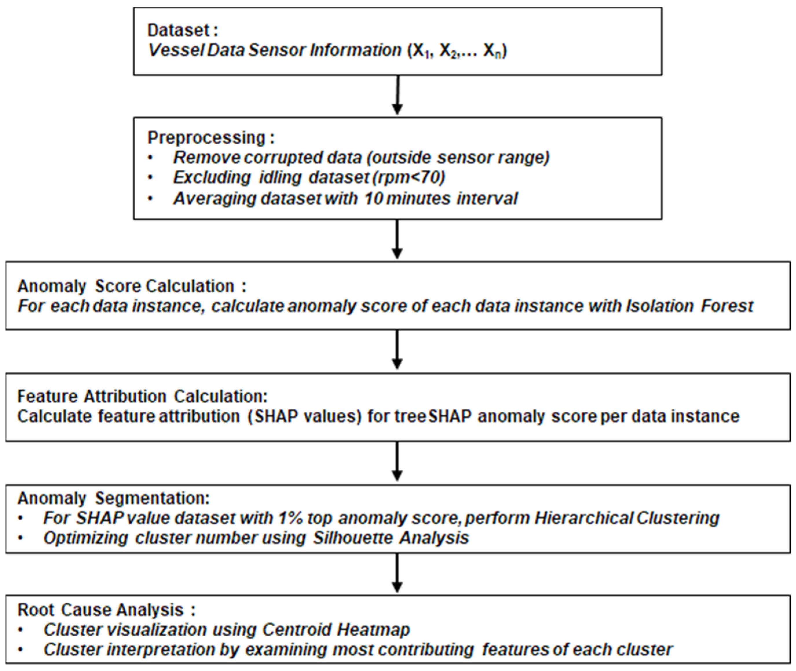
3.1. Overall Framework
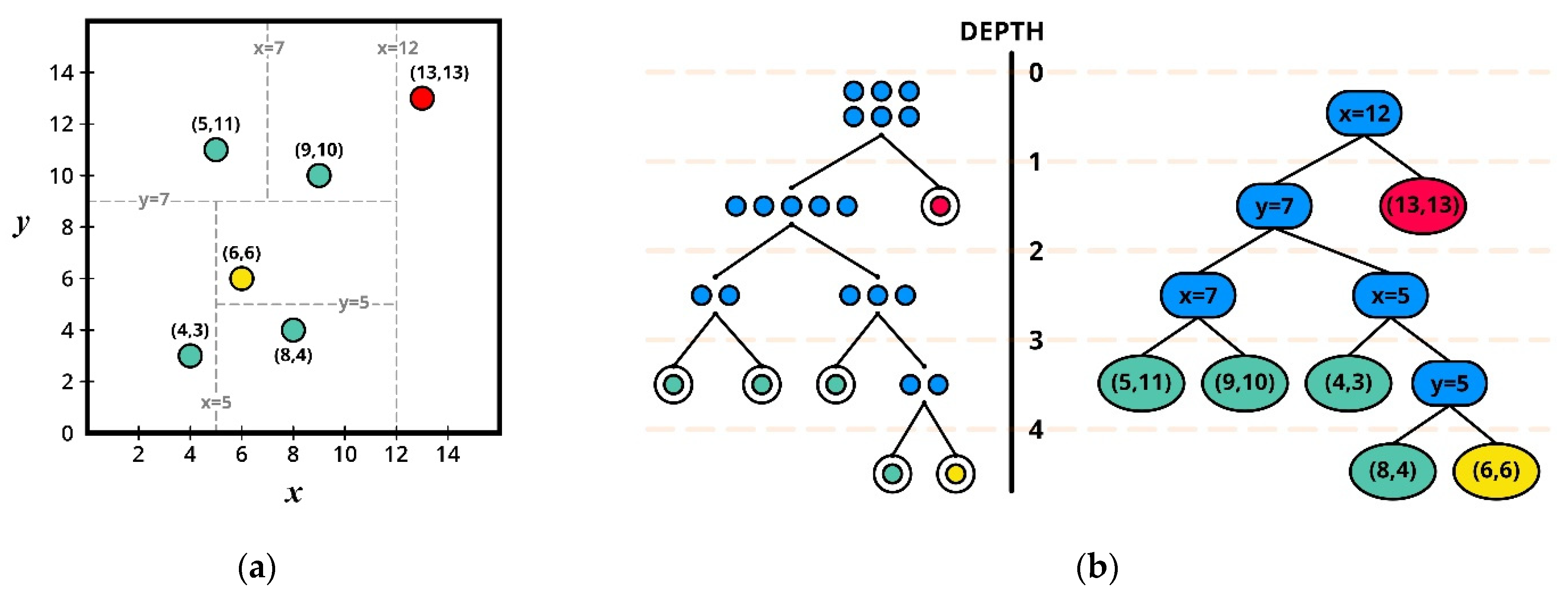
3.2. Unsupervised Anomaly Detection and Isolation Forest
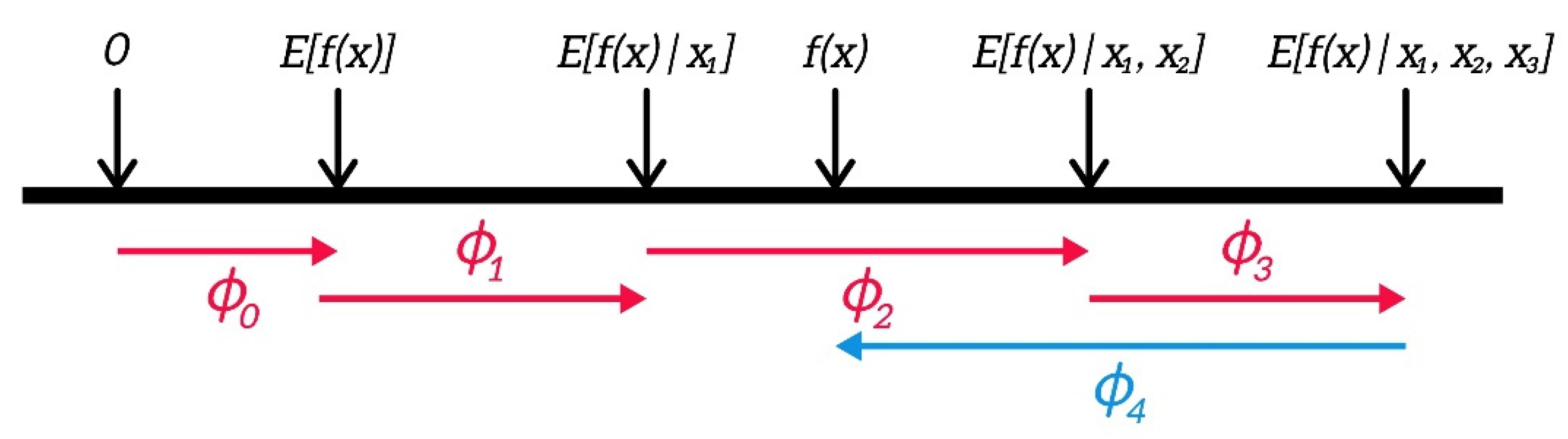
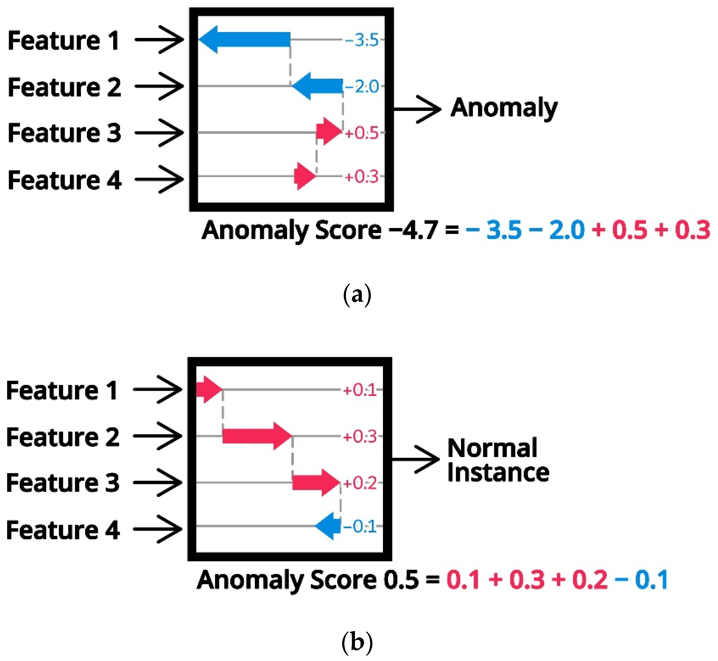
3.3. SHAP on Anomaly Detection
3.4. Hierarchical Clustering
4. Experiment Result and Discussion
4.1. Data Preprocessing
4.2. Anomaly Detection Using Isolation Forest
4.3. Feature Contribution Analysis Using SHAP
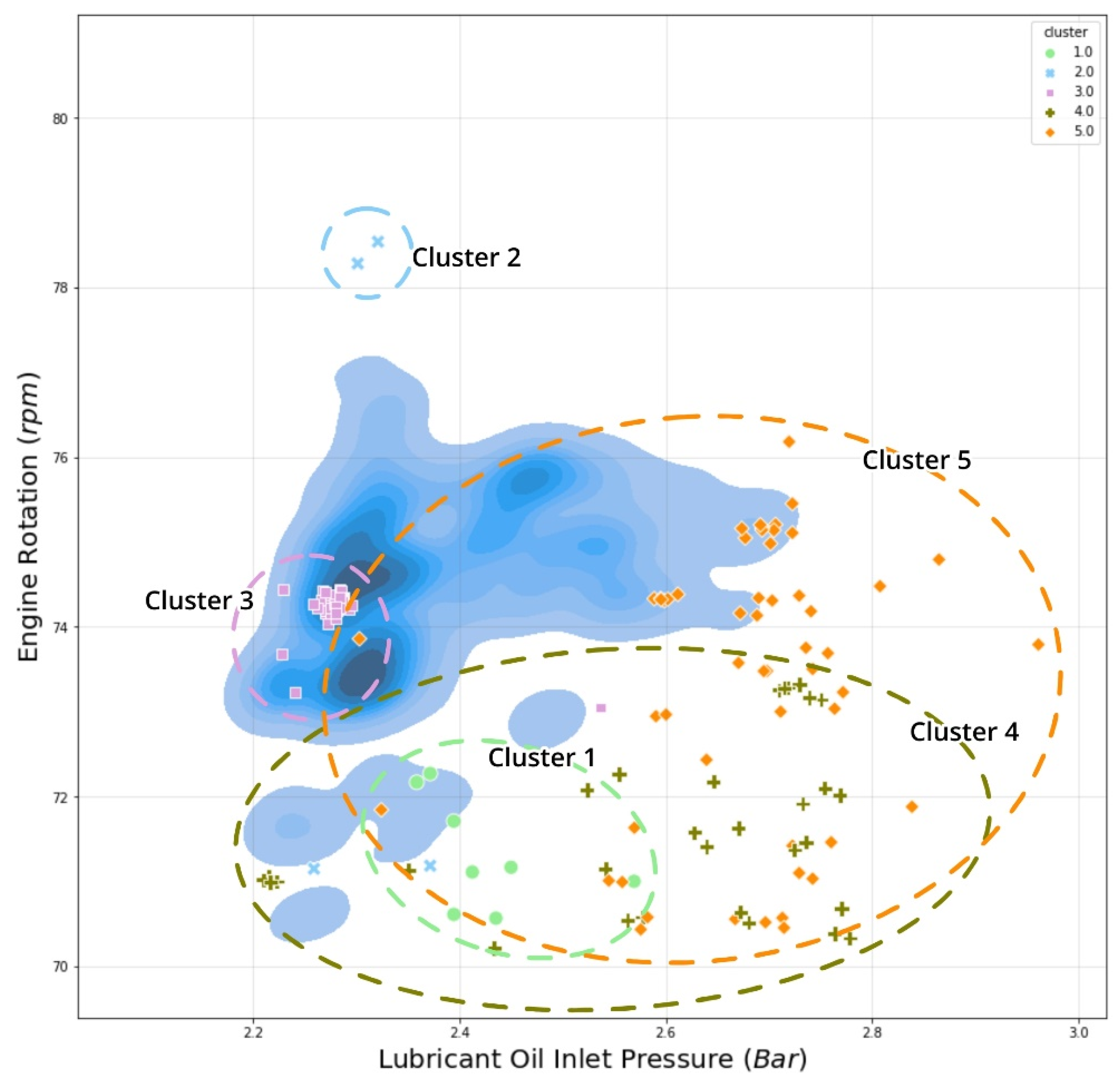
4.4. Anomalous Pattern Detection Using Hierarchical Clustering on Shapely Values
4.5. Discussion
5. Conclusions
Author Contributions
Funding
Conflicts of Interest
References
- Perera, L.P.; Mo, B. Data analysis on marine engine operating regions in relation to ship navigation. Ocean Eng. 2016, 128, 163–172. [Google Scholar] [CrossRef]
- Mirović, M.; Milicevic, M.; Obradović, I. Veliki skupovi podataka u pomorskoj industriji. Naše More 2018, 65, 56–62. [Google Scholar] [CrossRef]
- Gkerekos, C.; Lazakis, I.; Theotokatos, G. Machine learning models for predicting ship main engine Fuel Oil Consumption: A comparative study. Ocean Eng. 2019, 188, 106282. [Google Scholar] [CrossRef]
- Mak, L.; Sullivan, M.; Kuczora, A.; Millan, J. Ship performance monitoring and analysis to improve fuel efficiency. In 2014 Oceans-St. John’s; IEEE: Piscataway, NJ, USA, 2014; pp. 1–10. [Google Scholar] [CrossRef]
- Karagiannidis, P.; Themelis, N. Data-driven modelling of ship propulsion and the effect of data pre-processing on the prediction of ship fuel consumption and speed loss. Ocean Eng. 2021, 222, 108616. [Google Scholar] [CrossRef]
- Kim, D.; Lee, S.; Lee, J. Data-Driven Prediction of Vessel Propulsion Power Using Support Vector Regression with Onboard Measurement and Ocean Data. Sensors 2020, 20, 1588. [Google Scholar] [CrossRef] [PubMed] [Green Version]
- Gkerekos, C.; Lazakis, I. A novel, data-driven heuristic framework for vessel weather routing. Ocean Eng. 2020, 197, 106887. [Google Scholar] [CrossRef]
- Guanglei, L.; Hong, Z.; Dingyu, J.; Hao, W. Design of Ship Monitoring System Based on Unsupervised Learning. In International Conference on Intelligent and Interactive Systems and Applications; Springer: Berlin/Heidelberg, Germany, 2019; pp. 270–276. [Google Scholar] [CrossRef]
- Lazakis, I.; Dikis, K.; Michala, A.L.; Theotokatos, G. Advanced Ship Systems Condition Monitoring for Enhanced Inspection, Maintenance and Decision Making in Ship Operations. Transp. Res. Procedia 2016, 14, 1679–1688. [Google Scholar] [CrossRef] [Green Version]
- Beşikçi, E.B.; Arslan, O.; Turan, O.; Ölçer, A. An artificial neural network based decision support system for energy efficient ship operations. Comput. Oper. Res. 2016, 66, 393–401. [Google Scholar] [CrossRef] [Green Version]
- Filippopoulos, I.; Lajic, Z.; Mitsopoulos, G.; Senteris, A.; Pearson, M. Multi-Sensor Data Fusion for the Vessel Trim Analyzer and Optimization Platform. In Proceedings of the 2019 4th International Conference on System Reliability and Safety (ICSRS), Rome, Italy, 20–22 November 2019; IEEE: Piscataway, NJ, USA, 2019; pp. 35–40. [Google Scholar] [CrossRef]
- Jimenez, V.J.; Bouhmala, N.; Gausdal, A.H. Developing a predictive maintenance model for vessel machinery. J. Ocean Eng. Sci. 2020, 5, 358–386. [Google Scholar] [CrossRef]
- Diez-Olivan, A.; Pagan, J.A.; Sanz, R.; Sierra, B. Data-driven prognostics using a combination of constrained K-means clustering, fuzzy modeling and LOF-based score. Neurocomputing 2017, 241, 97–107. [Google Scholar] [CrossRef] [Green Version]
- Dikis, K.; Lazakis, I. Withdrawn: Dynamic predictive reliability assessment of ship systems. Int. J. Nav. Arch. Ocean Eng. 2019. [Google Scholar] [CrossRef]
- Obradović, I.; Miličević, M.; Žubrinić, K. Machine Learning Approaches to Maritime Anomaly Detection. NAŠE MORE Znanstveni Časopis za More i Pomorstvo 2014, 61, 96–101. Available online: https://hrcak.srce.hr/130339 (accessed on 31 July 2021).
- Kowalski, J.; Krawczyk, B.; Wozniak, M. Fault diagnosis of marine 4-stroke diesel engines using a one-vs-one extreme learning ensemble. Eng. Appl. Artif. Intell. 2017, 57, 134–141. [Google Scholar] [CrossRef]
- Cipollini, F.; Oneto, L.; Coraddu, A.; Murphy, A.J.; Anguita, D. Condition-based maintenance of naval propulsion systems: Data analysis with minimal feedback. Reliab. Eng. Syst. Saf. 2018, 177, 12–23. [Google Scholar] [CrossRef] [Green Version]
- Tan, Y.; Tian, H.; Jiang, R.; Lin, Y.; Zhang, J. A comparative investigation of data-driven approaches based on one-class classifiers for condition monitoring of marine machinery system. Ocean Eng. 2020, 201, 107174. [Google Scholar] [CrossRef]
- Vanem, E.; Brandsæter, A. Unsupervised anomaly detection based on clustering methods and sensor data on a marine diesel engine. J. Mar. Eng. Technol. 2019, 1–18. [Google Scholar] [CrossRef]
- Brandsæter, A.; Vanem, E.; Glad, I.K. Efficient on-line anomaly detection for ship systems in operation. Expert Syst. Appl. 2019, 121, 418–437. [Google Scholar] [CrossRef]
- Bae, Y.-M.; Kim, M.-J.; Kim, K.-J.; Jun, C.-H.; Byeon, S.-S.; Park, K.-M. A Case Study on the Establishment of Upper Control Limit to Detect Vessel’s Main Engine Failures using Multivariate Control Chart. J. Soc. Nav. Arch. Korea 2018, 55, 505–513. [Google Scholar] [CrossRef]
- Phaladiganon, P.; Kim, S.B.; Chen, V.C.P.; Baek, J.-G.; Park, S.-K. Bootstrap-BasedT2Multivariate Control Charts. Commun. Stat. Simul. Comput. 2011, 40, 645–662. [Google Scholar] [CrossRef]
- Mason, R.L.; Young, J.C. Multivariate Statistical Process Control with Industrial Applications; Society for Industrial and Applied Mathematics: University City, PA, USA, 2002. [Google Scholar]
- Kim, D.; Lee, S.; Lee, J. An Ensemble-Based Approach to Anomaly Detection in Marine Engine Sensor Streams for Efficient Condition Monitoring and Analysis. Sensors 2020, 20, 7285. [Google Scholar] [CrossRef]
- Ribeiro, M.T.; Singh, S.; Guestrin, C. “Why Should i Trust You?” Explaining the Predictions of Any Classifier. In Proceedings of the 22nd ACM SIGKDD International Conference on Knowledge Discovery and Data Mining, San Francisco, CA, USA, 13–17 August 2016; pp. 1135–1144. [Google Scholar] [CrossRef]
- Lundberg, S.; Lee, S.-I. A Unified Approach to Interpreting Model Predictions. In Proceedings of the 31st International Conference on Neural Information Processing Systems, Long Beach, CA, USA, 4–9 December 2017. [Google Scholar]
- Linardatos, P.; Papastefanopoulos, V.; Kotsiantis, S. Explainable AI: A Review of Machine Learning Interpretability Methods. Entropy 2020, 23, 18. [Google Scholar] [CrossRef]
- Wang, M.; Zheng, K.; Yang, Y.; Wang, X. An Explainable Machine Learning Framework for Intrusion Detection Systems. IEEE Access 2020, 8, 73127–73141. [Google Scholar] [CrossRef]
- Geschiere, V. Anomaly Detection for Predicting Failures in Waterpumping Stations; Vrije Universiteit: Amsterdam, The Netherland, 2020. [Google Scholar]
- Park, S.; Moon, J.; Hwang, E. Explainable Anomaly Detection for District Heating Based on Shapley Additive Explanations. In Proceedings of the 2020 International Conference on Data Mining Workshops (ICDMW), Sorrento, Italy, 17–20 November 2020; pp. 762–765. [Google Scholar] [CrossRef]
- Wong, C.W.; Chen, C.; Rossi, L.A.; Abila, M.; Munu, J.; Nakamura, R.; Eftekhari, Z. Explainable Tree-Based Predictions for Unplanned 30-Day Readmission of Patients With Cancer Using Clinical Embeddings. JCO Clin. Cancer Inform. 2021, 5, 155–167. [Google Scholar] [CrossRef]
- Lundberg, S.M.; Nair, B.; Vavilala, M.S.; Horibe, M.; Eisses, M.J.; Adams, T.; Liston, D.E.; Low, D.K.-W.; Newman, S.-F.; Kim, J.; et al. Explainable machine-learning predictions for the prevention of hypoxaemia during surgery. Nat. Biomed. Eng. 2018, 2, 749–760. [Google Scholar] [CrossRef]
- Liu, F.T.; Ting, K.M.; Zhou, Z.-H. Isolation-Based Anomaly Detection. ACM Trans. Knowl. Discov. Data 2012, 6, 1–39. [Google Scholar] [CrossRef]
- Cheliotis, M.; Lazakis, I.; Theotokatos, G. Machine learning and data-driven fault detection for ship systems operations. Ocean Eng. 2020, 216, 107968. [Google Scholar] [CrossRef]
- MAN Two Stroke—Project Guide. (n.d.). Available online: https://marine.man-es.com/two-stroke/project-guides (accessed on 16 April 2021).
- Breunig, M.M.; Kriegel, H.-P.; Ng, R.T.; Sander, J. LOF: Identifying Density-Based Local Outliers. In Proceedings of the SIGMOD ’00: Proceedings of the 2000 ACM SIGMOD International Conference on Management of Data, New York, NY, USA, 16 May 2000; pp. 93–104. [CrossRef]
- Angiulli, F.; Pizzuti, C. Fast Outlier Detection in High Dimensional Spaces. In PKDD 2002: Principles of Data Mining and Knowledge Discovery; Springer: Berlin/Heidelberg, Germany, 2002; pp. 15–27. [Google Scholar] [CrossRef] [Green Version]
- Goldstein, M.; Dengel, A. Histogram-Based Outlier Score (HBOS): A Fast Unsupervised Anomaly Detection Algorithm. In KI-2012: Poster and Demo Track; Wölfl, S., Ed.; Citeseer: Princeton, NJ, USA, 2012; pp. 59–63. [Google Scholar]
- Almardeny, Y.; Boujnah, N.; Cleary, F. A Novel Outlier Detection Method for Multivariate Data. IEEE Trans. Knowl. Data Eng. 2020. [Google Scholar] [CrossRef]
- Kriegel, H.-P.; Hubert, M.S.; Zimek, A. Angle-based outlier detection in high-dimensional data. In Proceedings of the KDD ’08: Proceedings of the 14th ACM SIGKDD International Conference on Knowledge Discovery and Data Mining, Las Vegas, NV, USA, 24–27 August 2008; pp. 444–452. [CrossRef] [Green Version]
- Li, Z.; Zhao, Y.; Botta, N.; Ionescu, C.; Hu, X. COPOD: Copula-Based Outlier Detection; IEEE: Piscataway, NJ, USA, 2020; pp. 1118–1123. [Google Scholar] [CrossRef]
- Zhao, Y.; Nasrullah, Z.; Hryniewicki, M.K.; Li, Z. LSCP: Locally Selective Combination in Parallel Outlier Ensembles. In Proceedings of the 2019 SIAM International Conference on Data Mining (SDM), Calgary, AB, Canada, 2–4 May 2019; pp. 585–593. [Google Scholar] [CrossRef] [Green Version]
- Pevný, T. Loda: Lightweight on-line detector of anomalies. Mach. Learn. 2015, 102, 275–304. [Google Scholar] [CrossRef] [Green Version]
- Aggarwal, C.C. An Introduction to Outlier Analysis. In Outlier Analysis; Springer: Berlin/Heidelberg, Germany, 2016; pp. 1–34. [Google Scholar] [CrossRef]
- Liu, F.T.; Ting, K.M.; Zhou, Z.-H. Isolation Forest; IEEE: Piscataway, NJ, USA, 2008; pp. 413–422. [Google Scholar] [CrossRef]
- Roth, A.E. The Shapley Value: Essays in Honor of Lloyd S Shapley; Cambridge University Press: Cambridge, UK, 1988. [Google Scholar]
- Lundberg, S.M.; Erion, G.G.; Lee, S.I. Consistent individualized feature attribution for tree ensembles. arXiv 2018, arXiv:1802.03888. [Google Scholar]
- Lundberg, S.M.; Erion, G.; Chen, H.; DeGrave, A.; Prutkin, J.M.; Nair, B.; Katz, R.; Himmelfarb, J.; Bansal, N.; Lee, S.-I. From local explanations to global understanding with explainable AI for trees. Nat. Mach. Intell. 2020, 2, 56–67. [Google Scholar] [CrossRef]
- Ding, F.; Wang, J.; Ge, J.; Li, W. Anomaly detection in large-scale trajectories using hybrid grid-based hierarchical clustering. Int. J. Robot. Autom. 2018, 33. [Google Scholar] [CrossRef] [Green Version]
- Rousseeuw, P.J. Silhouettes: A graphical aid to the interpretation and validation of cluster analysis. J. Comput. Appl. Math. 1987, 20, 53–65. [Google Scholar] [CrossRef] [Green Version]
- Saputra, D.M.; Saputra, D.; Oswari, L.D. Effect of Distance Metrics in Determining K-Value in K-Means Clustering Using Elbow and Silhouette Method. In Advances in Intelligent Systems Research; Atlantis Press: Palembang, Indonesia, 2020; pp. 341–346. [Google Scholar] [CrossRef]
- Project Guides Electronically Controlled Two-stroke Engine; MAN Energy Solutions: Augsburg, Germany, 2021.
- Huang, Y.; Hong, G. Investigation of the effect of heated ethanol fuel on combustion and emissions of an ethanol direct injection plus gasoline port injection (EDI + GPI) engine. Energy Convers. Manag. 2016, 123, 338–347. [Google Scholar] [CrossRef]
- Rubio, J.A.P.; Vera-García, F.; Grau, J.H.; Cámara, J.M.; Hernandez, D.A. Marine diesel engine failure simulator based on thermodynamic model. Appl. Therm. Eng. 2018, 144, 982–995. [Google Scholar] [CrossRef]


| Specification | |
|---|---|
| Length overall | 269.36 m |
| Length between perpendiculars | 259.00 m |
| Breadth | 43.00 m |
| Depth | 23.80 m |
| Draught | 17.30 m |
| Deadweight | 152.517 metric t |
| Feature Name | Description |
|---|---|
| TIME_STAMP | A time when the data is recorded |
| ME1_FO_TEMP_INLET | Temperature of fuel oil |
| ME1_RPM | Engine rotation per minute (RPM) |
| ME1_FO_INLET_PRESS | Inlet pressure of fuel oil |
| ME1_FO_INLET_TEMP | Inlet temperature of fuel oil |
| ME1_SCAV_AIR_PRESS | Pressure of scavenging air |
| ME1_JCW_INLET_TEMP | Inlet temperature of jacket cooling water |
| ME1_JCW_INLET_PRESS | Inlet pressure of jacket cooling water |
| ME1_TC1_EXH_INLET_TEMP | Inlet temperature of exhaust gas of turbocharger |
| ME1_TC1_EXH_OUTLET_TEMP | Outlet temperature of exhaust gas of turbocharger |
| ME1_TC1_LO_INLET_PRESS | Inlet pressure of lubricant oil in turbocharger |
| ME1_TC1_LO_OUTLET_TEMP | Outlet temperature of lubricant oil in turbocharger |
| ME1_LO_INLET_PRESS | Inlet pressure of lubricant oil |
| ME1_LO_INLET_TEMP | Inlet temperature of lubricant oil |
| ME1_CYL [1~5]_PCO_OUTLET_TEMP | Outlet temperature of cylinder piston cooling oil (cylinders 1 to 5) |
| ME1_CYL [1~5]_CFW_OUTLET_TEMP | Outlet temperature of cylinder block cooling water (cylinders 1 to 5) |
| ME1_CYL [1~5]_EXH_GAS_OUTLET_TEMP | Outlet temperature of exhaust gas (cylinders 1 to 5) |
| Feature Name | Anomalous Instances | Normal Instances |
|---|---|---|
| 12 September 2019 (7:10 KST) | 21 October 2019 (13:50 KST) | |
| ME1_RPM | 74.279 | 73.644 |
| ME1_FO_INLET_PRESS | 7.473 | 6.901 |
| ME1_FO_INLET_TEMP | 142.913 | 138.045 |
| ME1_SCAV_AIR_PRESS | 1.576 | 1.343 |
| ME1_JCW_INLET_TEMP | 76.800 | 71.670 |
| ME1_JCW_INLET_PRESS | 3.727 | 3.646 |
| ME1_TC1_LO_INLET_PRESS | 1.973 | 2.048 |
| ME1_TC1_LO_OUTLET_TEMP | 68.908 | 57.647 |
| ME1_LO_INLET_PRESS | 2.279 | 2.363 |
| ME1_LO_INLET_TEMP | 54.290 | 45.948 |
| ME1_CYL_PCO_OUTLET_TEMP | 59.117 | 50.787 |
| ME1_CYL_CFW_OUTLET_TEMP | 84.867 | 78.983 |
| ME1_CYL_EXH_GAS_OUTLET_TEMP | 354.501 | 341.918 |
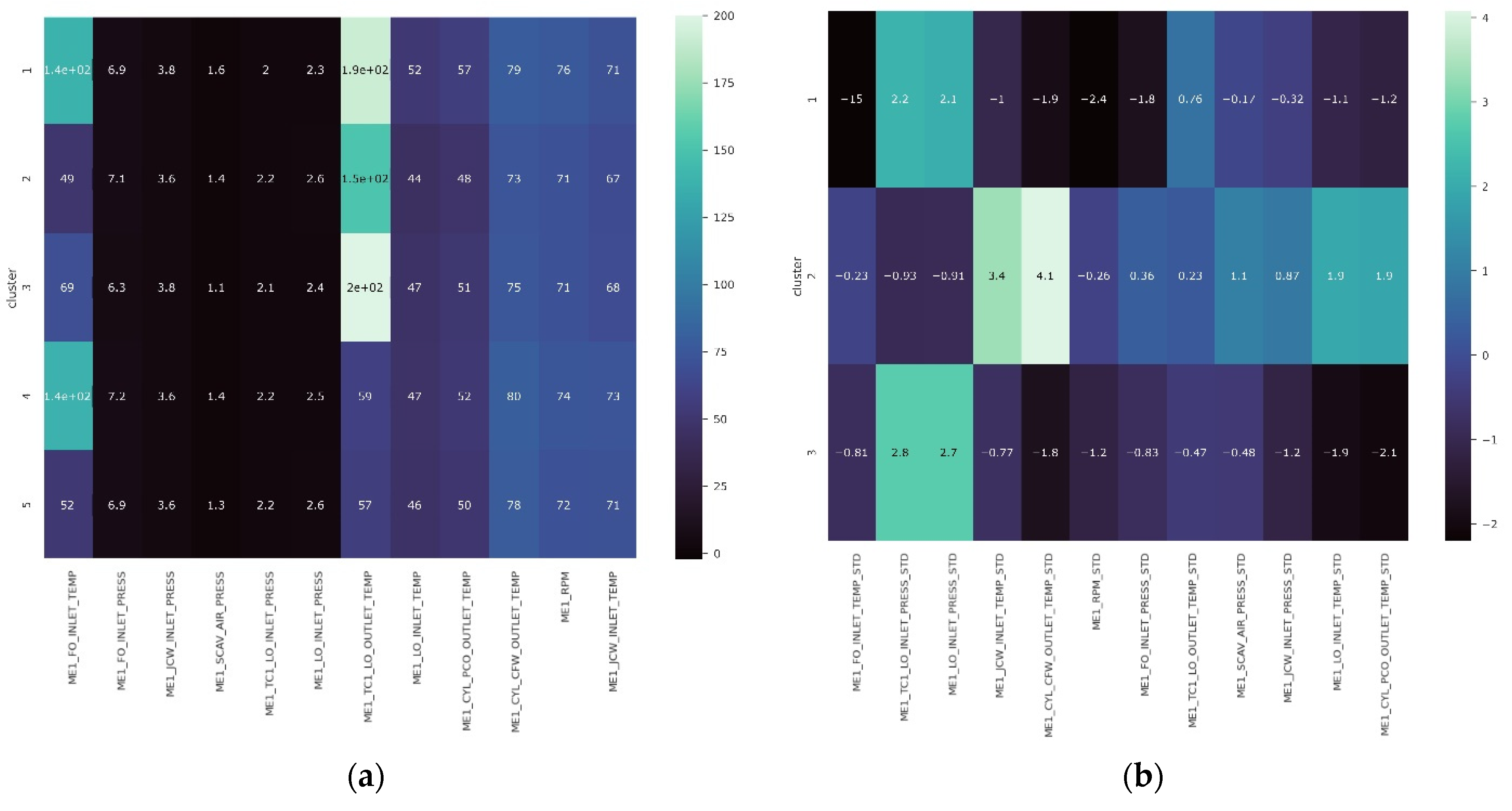
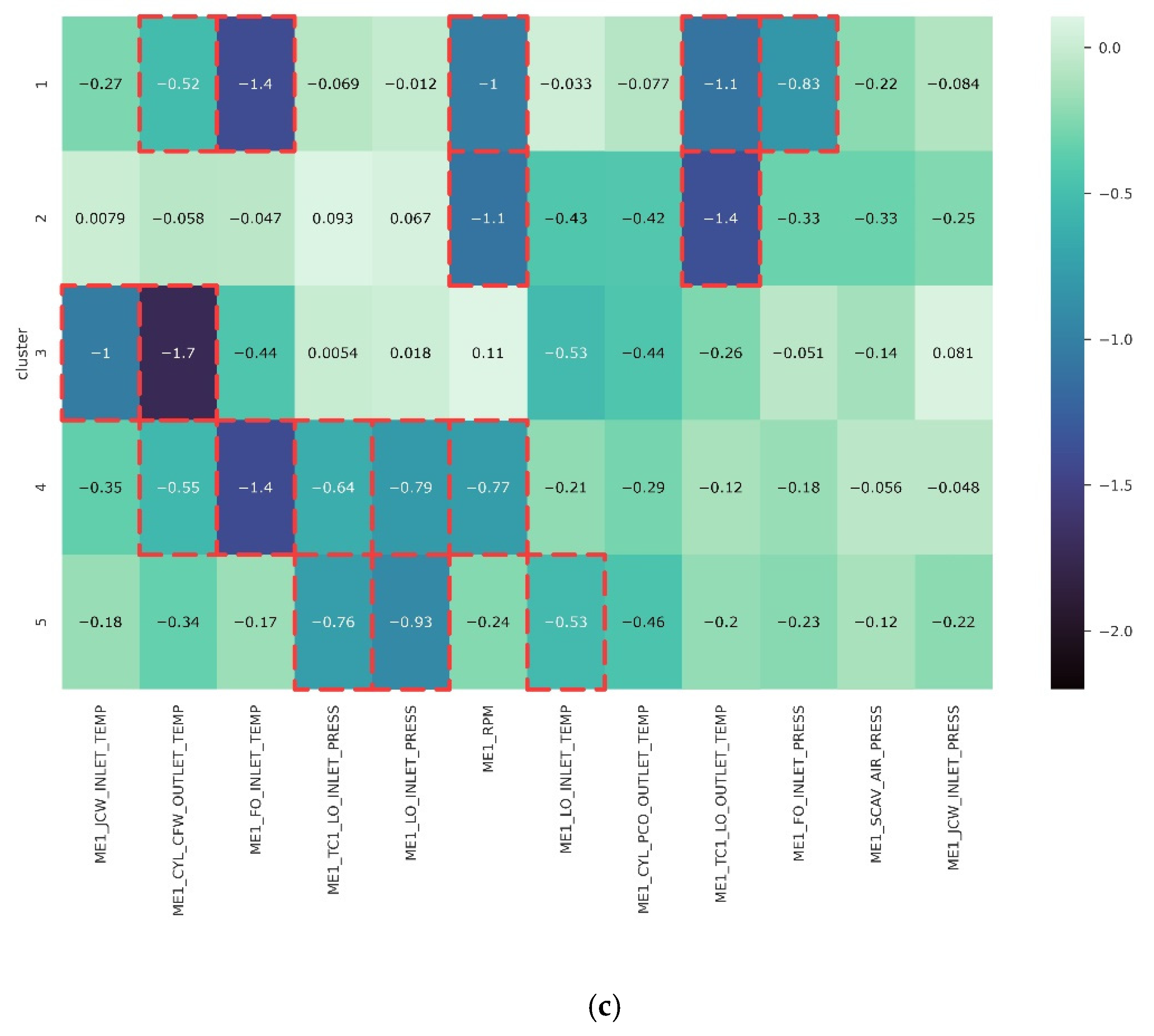
| Parameters | Actual Value Dataset (a) | Standardized Dataset (b) | SHAP Value Dataset (c) |
|---|---|---|---|
| Feature importance | ✗ | ✗ | ✓ |
| Instance scoring | ✗ | ✗ | ✓ |
| Detect anomaly on the same subquartile | ✗ | ✓ | ✓ |
| Detect anomaly on contradictory quartile region | ✗ | ✗ | ✓ |
| Heatmap result segmentation | ✓ | ✓ | ✓ |
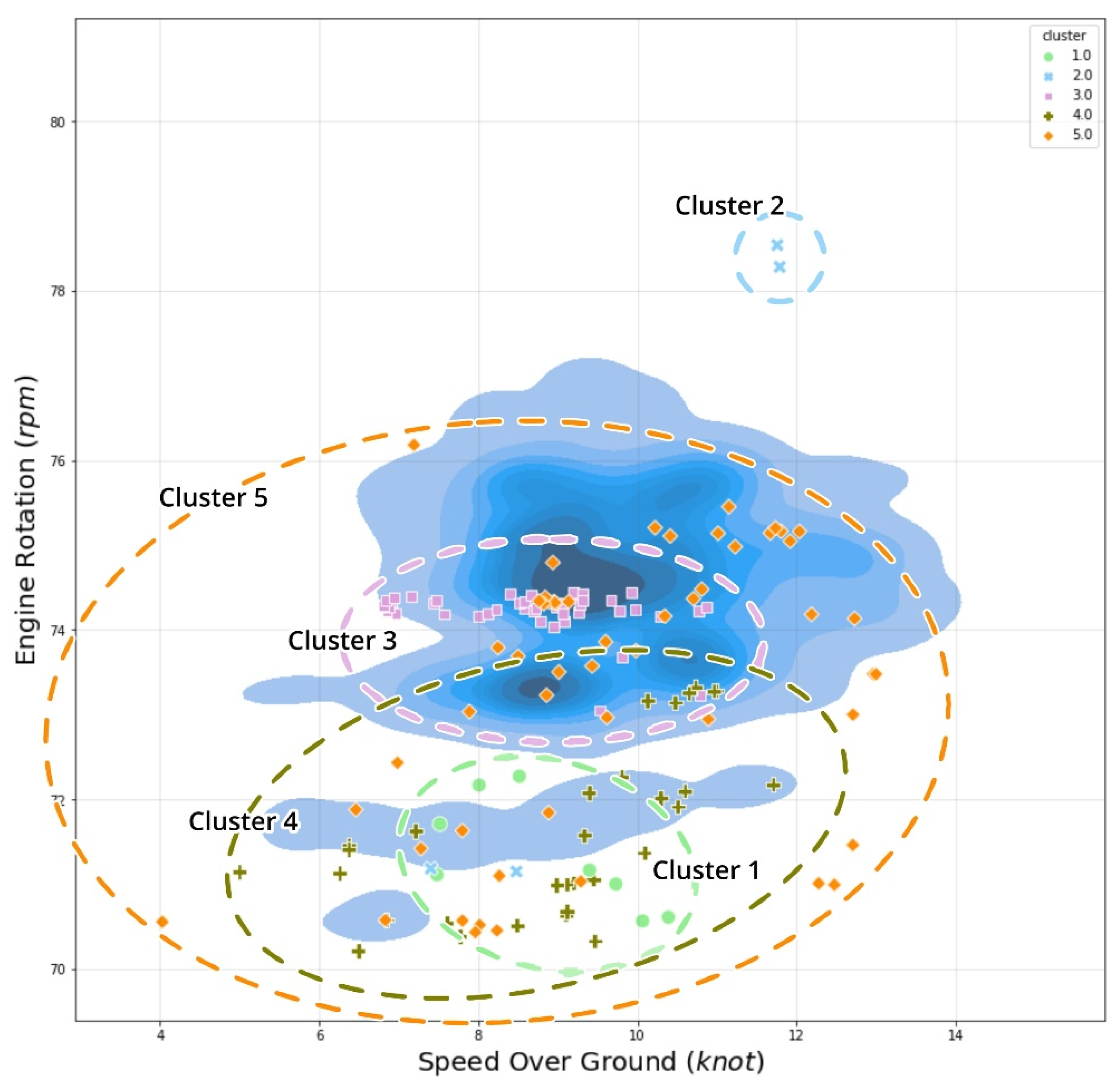
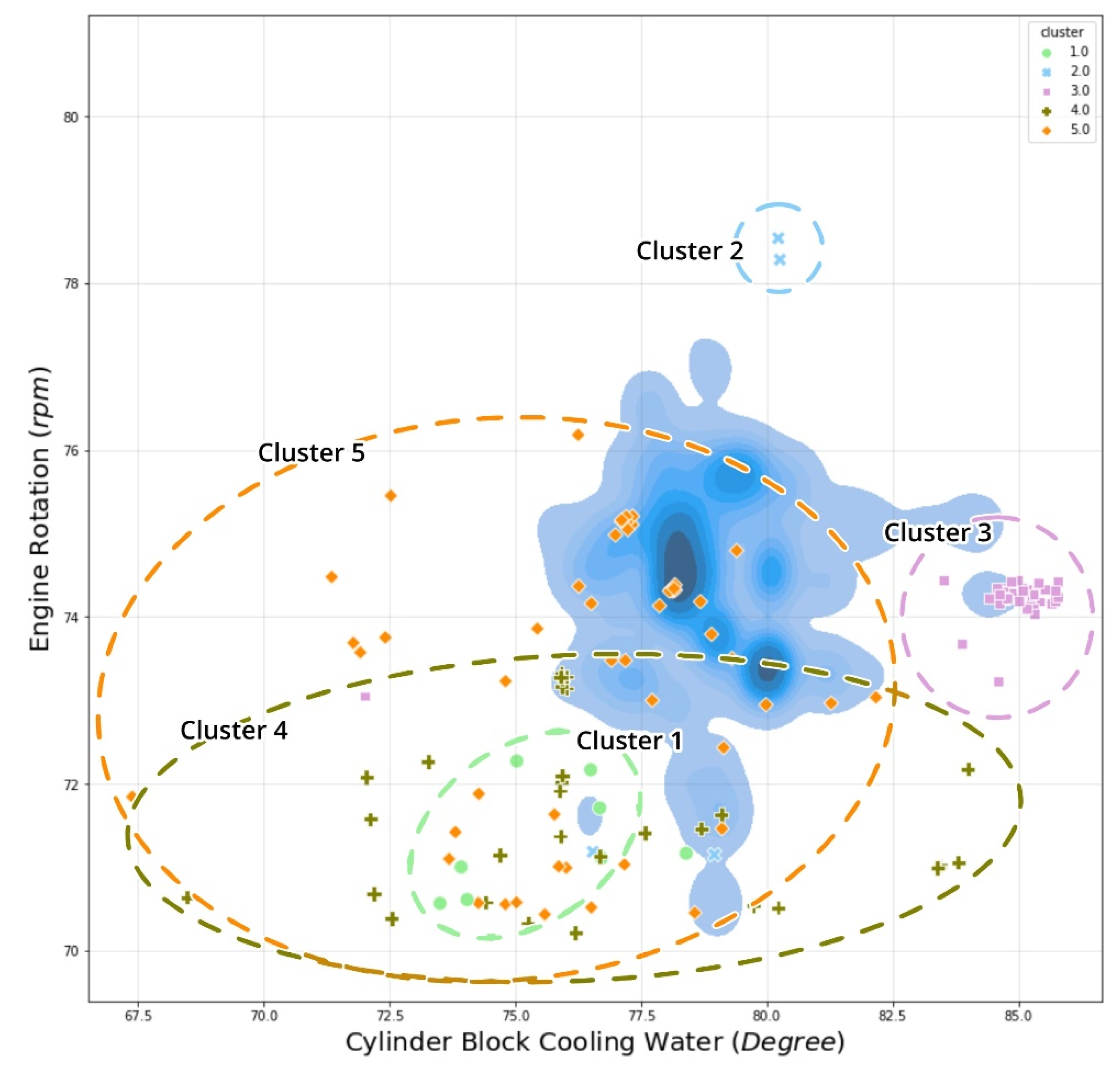
| Clusters | Anomalous Features | Description | Vessel Status |
|---|---|---|---|
| Cluster 1 | ME1_CYL_CFW_OUTLET_TEMP | Intermediate to a low temperature of cylinder block cooling water | (Deceleration; suspicious temperature rate) Docking to the port MCR 55–57% Deceleration/acceleration |
| ME1_FO_INLET_TEMP | Low inlet temperature of fuel oil | ||
| ME1_RPM | Low engine rotation per minute (RPM) | ||
| ME1_TC1_LO_OUTLET_TEMP | Extreme high outlet turbocharger temperature of lubricant oil | ||
| ME1_FO_INLET_PRESS | Extreme low inlet pressure of fuel oil | ||
| Cluster 2 | ME1_RPM | High engine rotation per minute (RPM) | (Overly high performance) High cruise speed (>10 knots) MCR > 60% |
| ME1_TC1_LO_OUTLET_TEMP | Extreme high outlet turbocharger Temperature of lubricant oil | ||
| Cluster 3 | ME1_JCW_INLET_TEMP | High inlet temperature of jacket cooling water | (High performance constantly) Cruise speed MCR 58% |
| ME1_CYL_CFW_OUTLET_TEMP | High temperature of cylinder block cooling water | ||
| ME1_LO_INLET_TEMP | High inlet temperature of lubricant oil | ||
| Cluster 4 | ME1_CYL_CFW_OUTLET_TEMP | Intermediate to a low temperature of cylinder block cooling water | (Deceleration; suspicious pressure rate) Docking to the port or Slow ahead MCR 54–58% Deceleration/acceleration |
| ME1_FO_INLET_TEMP | Extreme low inlet temperature of fuel oil | ||
| ME1_TC1_LO_INLET_PRESS | Intermediate to high outlet turbocharger pressure of lubricant oil | ||
| ME1_LO_INLET_PRESS | Intermediate to high inlet pressure of lubricant oil | ||
| ME1_RPM | Low engine rotation per minute (RPM) | ||
| Cluster 5 | ME1_TC1_LO_INLET_PRESS | High turbocharger inlet pressure of lubricant oil | (Overcooling engine) Slow ahead MCR 55–60% Possibility engine start |
| ME1_LO_INLET_PRESS | Intermediate to high inlet pressure of lubricant oil | ||
| ME1_LO_INLET_TEMP | Low to extreme low inlet temperature of lubricant oil |
Publisher’s Note: MDPI stays neutral with regard to jurisdictional claims in published maps and institutional affiliations. |
© 2021 by the authors. Licensee MDPI, Basel, Switzerland. This article is an open access article distributed under the terms and conditions of the Creative Commons Attribution (CC BY) license (https://creativecommons.org/licenses/by/4.0/).
Share and Cite
Kim, D.; Antariksa, G.; Handayani, M.P.; Lee, S.; Lee, J. Explainable Anomaly Detection Framework for Maritime Main Engine Sensor Data. Sensors 2021, 21, 5200. https://doi.org/10.3390/s21155200
Kim D, Antariksa G, Handayani MP, Lee S, Lee J. Explainable Anomaly Detection Framework for Maritime Main Engine Sensor Data. Sensors. 2021; 21(15):5200. https://doi.org/10.3390/s21155200
Chicago/Turabian StyleKim, Donghyun, Gian Antariksa, Melia Putri Handayani, Sangbong Lee, and Jihwan Lee. 2021. "Explainable Anomaly Detection Framework for Maritime Main Engine Sensor Data" Sensors 21, no. 15: 5200. https://doi.org/10.3390/s21155200
APA StyleKim, D., Antariksa, G., Handayani, M. P., Lee, S., & Lee, J. (2021). Explainable Anomaly Detection Framework for Maritime Main Engine Sensor Data. Sensors, 21(15), 5200. https://doi.org/10.3390/s21155200