Communication

Predicting Pressure Sensitivity to Luminophore Content and Paint Thickness of Pressure-Sensitive Paint Using Artificial Neural Network

1
Department of Aerospace and Mechanical Engineering, University of Notre Dame, Notre Dame, IN 46556, USA
2
Department of Mechanical Engineering, Aichi Institute of Technology, 1247 Yachigusa, Yakusa-cho, Toyota 470-0392, Aichi, Japan
*
Author to whom correspondence should be addressed.
Sensors 2021, 21(15), 5188; https://doi.org/10.3390/s21155188
Submission received: 28 June 2021 / Revised: 25 July 2021 / Accepted: 28 July 2021 / Published: 30 July 2021
(This article belongs to the Special Issue Optical Sensors for Flow Diagnostics)

Abstract

:
An artificial neural network (ANN) was constructed and trained for predicting pressure sensitivity using an experimental dataset consisting of luminophore content and paint thickness as chemical and physical inputs. A data augmentation technique was used to increase the number of data points based on the limited experimental observations. The prediction accuracy of the trained ANN was evaluated by using a metric, mean absolute percentage error. The ANN predicted pressure sensitivity to luminophore content and to paint thickness, within confidence intervals based on experimental errors. The present approach of applying ANN and the data augmentation has the potential to predict pressure-sensitive paint (PSP) characterizations that improve the performance of PSP for global surface pressure measurements.

1. Introduction

Pressure-sensitive paint (PSP) using a luminophore has been widely used as pressure sensor in fluid dynamics studies [1,2,3,4]. A key feature of PSP is the sensitivity to pressure variations [5,6,7,8,9,10,11]. The luminescence of the PSP is converted to pressure using the Stern–Volmer equation [11]. Given the relationship between the luminescence of the PSP and corresponding pressure, a PSP with higher pressure sensitivity is desirable.
The higher pressure sensitivity is obtained by adjusting the paint formulation of the PSP. The luminophore concentration of the PSP influences the pressure sensitivity [11,12,13]. Other components such as the thickness of the PSP applied to a surface also affect the pressure sensitivity [14,15,16,17]. The pressure sensitivity of the PSP is determined by an experimental calibration. Typically, one component of a PSP is varied at a time to extract the correlation between the component and pressure sensitivity. Depending on the range of required pressure sensitivity, an extensive range of the components sensitive to pressure sensitivity must be experimentally investigated. Such investigations require significant time since many experimental coupons must be created and calibrated. Ideally, all components must be investigated, including their mutual interactions, in order to map their influence on the pressure sensitivity of the PSP. Given the complex nature of the correlations between the pressure sensitivity and components, it is challenging to incorporate all of the components into a parametric study due to experimental time constraints. It is highly desirable to create a model linking the pressure sensitivity and components related to the PSP. In this work, we investigate the use of artificial neural networks (ANNs) to create the model.
ANNs are often used to approximate nonlinear functions with great success in various fields including chemical engineering [18,19,20], civil engineering [21,22], electrical engineering [23], computer engineering [24], and interdisciplinary engineering [25,26,27,28,29,30,31]. In this work, the ANN is applied to predictions of the pressure sensitivity of a PSP. The ANN architecture is constructed and trained using the PSP datasets measured. A practical challenge is that the prediction accuracy of the ANN depends on the number of data points [32]. Large datasets reduce overfitting and generalize the ANN predictive capabilities [32,33,34,35] However, due to the extensive time required for experiments, the number of data points measured is typically small, consisting of less than a hundred data points. Data augmentation techniques are often used to increase the number of data points [36].
In the present paper, we study the suitability of the use of an ANN in predicting the pressure sensitivity of the PSP to luminophore content and paint thickness. The ANN is used instead of typical approaches such as phenomenological modeling or statistical modeling approaches. The correlation among the three parameters is hard to obtain by the typical approaches because the phenomenon that determines pressure sensitivity is coupled by chemical and physical factors. As components increase, the application of typical approaches becomes increasingly difficult. The main goal of the present study is to enable the replacement of time-consuming and expensive experiments by an ANN trained to predict pressure sensitivity to given components related to PSP. To the best of our knowledge, the present study is the first attempt to apply an ANN to PSP development. The ANN is trained using an experimental dataset to obtain the correlation between pressure sensitivity with luminophore content and paint thickness. The training dataset includes the following variables: paint thickness (mm), luminophore content (mg), and pressure sensitivity (%/kPa). This paper also investigates the general applicability of the ANN trained using an augmented dataset utilizing experimental errors. The data augmentation technique is used to increase the number of data points from experimental observations.

2. Experimental and Augmented Dataset

An experimental dataset was used to train an ANN and evaluate the prediction performance of the trained ANN. The experimental dataset was collected through the characterization of PSP coupons. Luminophore content and paint thickness are mutually independent variables, and they are chemical and physical factors that impact pressure sensitivity, respectively. The luminophore content and paint thickness of PSP coupons were selected to design a PSP that increases the pressure sensitivity as much as possible. The pressure sensitivity was obtained for different luminophore contents and paint thicknesses. The experimental dataset, DO, consisting of a total of 84 measurements, was split into 90% for the training dataset; DO,76, composed of 76 data points and 10% for the test dataset; and DO,8, consisting of 8 data points. Typically, 80% and 20% of data points or 90% and 10% of data points are used for training and testing, respectively. The present study selected the latter ratio to increase the training dataset because the available experimental data is limited to less than 100 points. Table 1 shows the range and the experimental errors of the experimental dataset for PSP coupons. Details of the collection of experimental datasets are described in Appendix A.
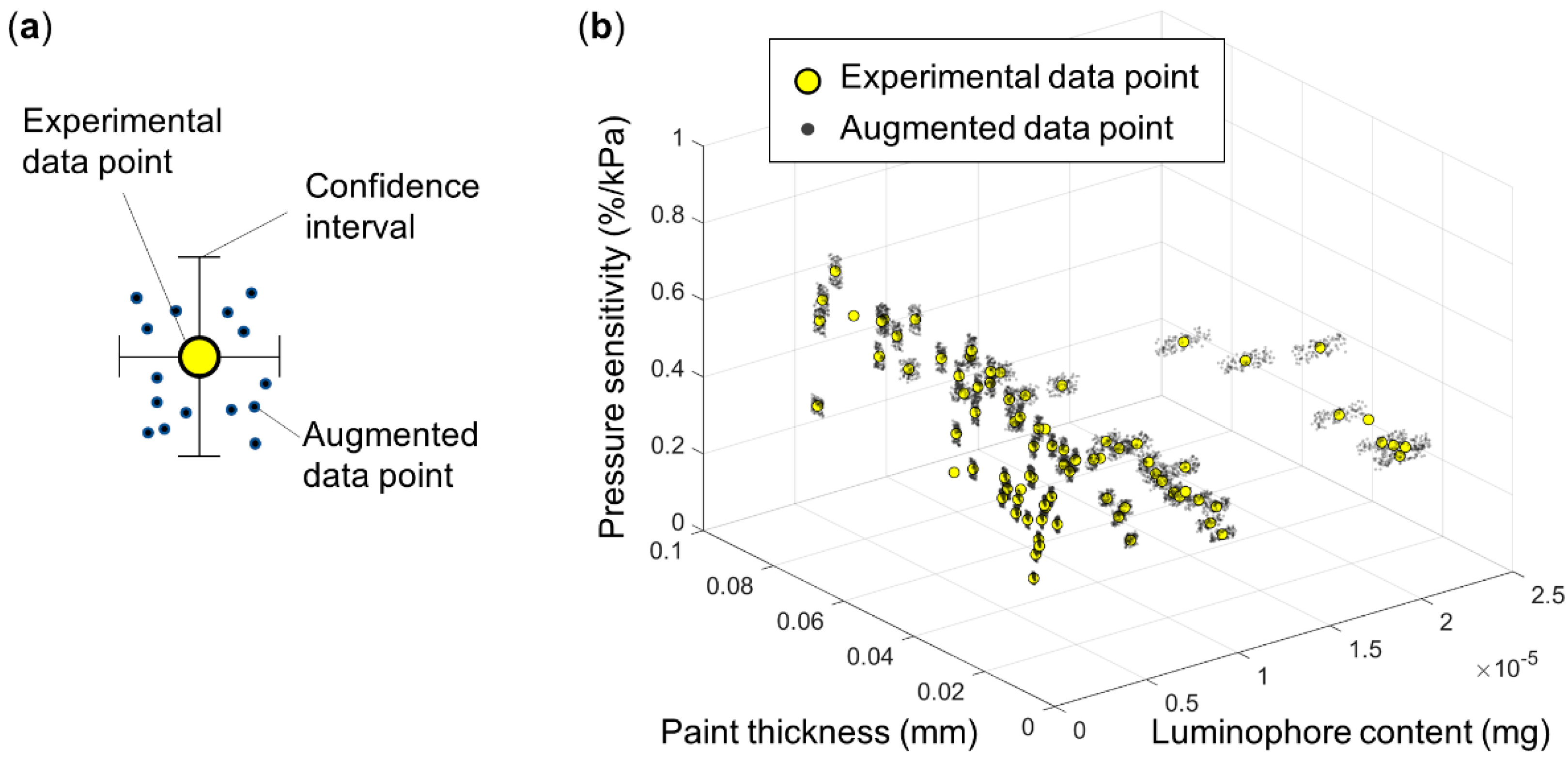
The augmented dataset, DA, was used to train the ANN. The augmented dataset was produced using the experimental dataset. Figure 1a shows the schematic concept of the data augmentation used in the present study. The data augmentation produced the data points distributed within the confidence intervals based on experimental errors at each observation point. Here, it is assumed that there is no correlation between the error and the variable (i.e., all variables are mutually independent). The randomness of the dataset produced by the data augmentation follows a Gaussian distribution centered at zero. The data augmentation produced data, DA,n, consisting of 76, 760, 7600, 76,000, and 760,000 entries starting from the training dataset, DO,76, with 76 data points. The subscript n in DA,n, indicates the total number of entries obtained through the augmentation procedure. The number of augmented data points was varied to find the one that yields the most accurate ANN model. Figure 1(b) shows an example of the augmented dataset, DA,7600, with 7600 data points created around each observation point. The data augmentation process is repeated for each experimentally observed data point corresponding to various paint thicknesses and luminophore contents.
Dataset standardization was performed to avoid numerical issues and avoid divergence of the training process during the training caused by different input scales in a dataset with differing physical units and values [37]. Standardization of the dataset was achieved by normalization using the mean and standard deviation.

3. ANN Model Development

3.1. Architecture of ANN Models

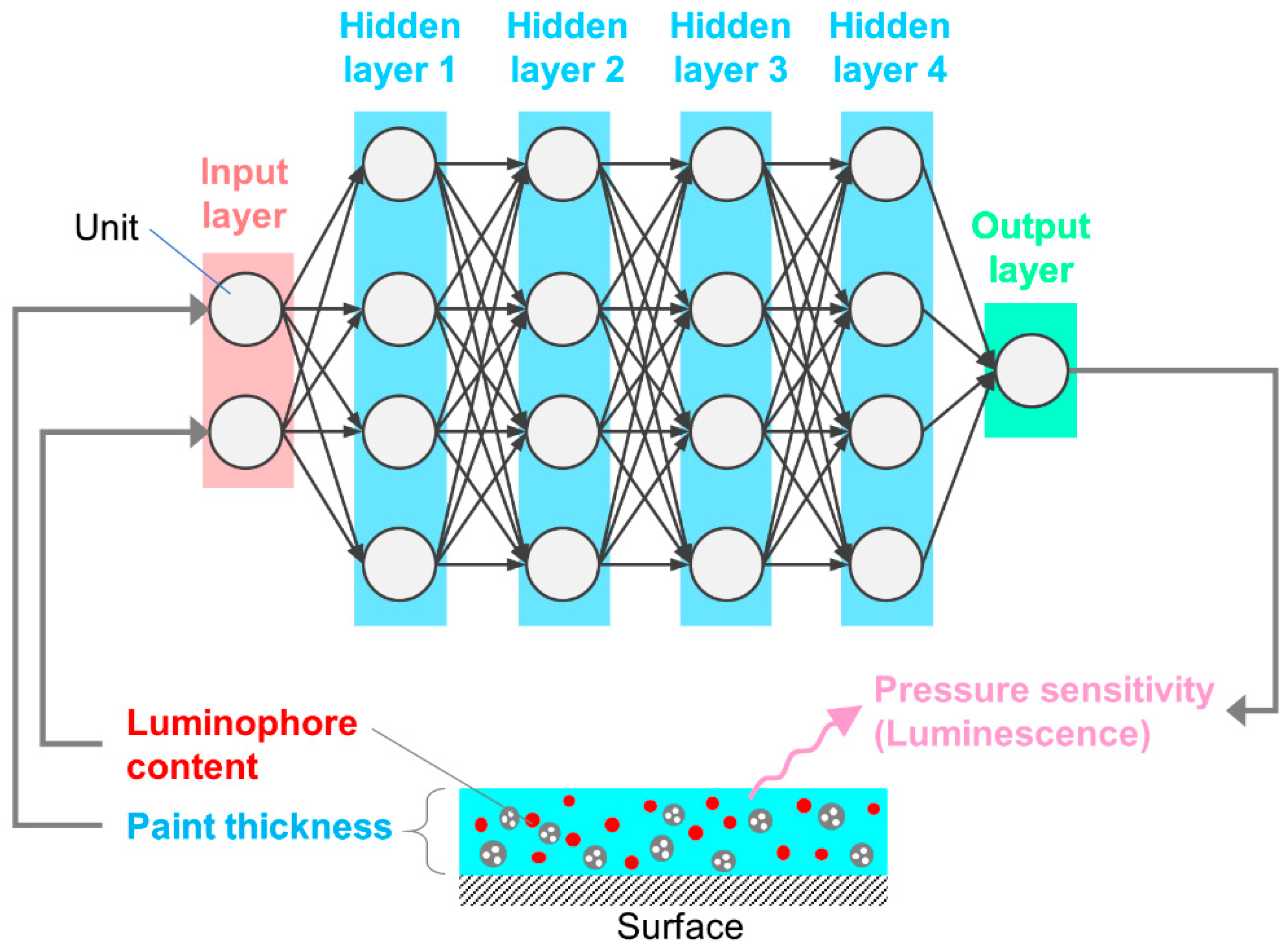
Figure 2 shows the schematic description of the architecture of the ANN model used in the present study. The architecture was realized through a fully connected, deep ANN consisting of the input layer with two units, the hidden layers with four units, and the output layer with a single unit. Here, units are also called neurons in terms of a biological brain. Luminophore content and paint thickness are considered to constitute inputs of the ANN models, while the pressure sensitivity constituted an output of the ANN models. The activation function, rectified linear unit (ReLU), was used in the hidden layers [38]. Further details regarding the architecture and studies used to define the final architecture are provided in Appendix B. The selected architecture of the ANN model is summarized in Figure 2.

3.2. Training of ANN Models

ANN models were trained using the augmented datasets, DA,n. An ANN model was also trained using the experimental training dataset, DO,76, in order to compare with the ANN models trained by augmented datasets. The ANN models were trained for 40,000 epochs. The ANN model weights were optimized using the Adam optimizer [39]. Because the random selection of the initial ANN model weights in the training influences updated weights, resulting in different predictions, each ANN model was trained 10 times to obtain the median. The learning rate was set at 10−3. Table 2 summarizes the ANN models for different training datasets.

4. Evaluation of the Prediction Performance of Trained ANN Models

The performance of the trained ANN models was assessed by the accuracy of the prediction of the ANN models when the test dataset, DO,8, was used. A metric, mean absolute percentage error (MAPE), was used in quantitatively assessing the accuracy of the predictions [40,41]. The MAPE was calculated using the following equation [40,42]:
MAPE % = 1 N i = 1 N | o i p i | o i × 100 .
Here, oi is the vector of observed values, pi is the vector of predicted values, i is the index, and N is the number of data points.

5. Results and Discussion

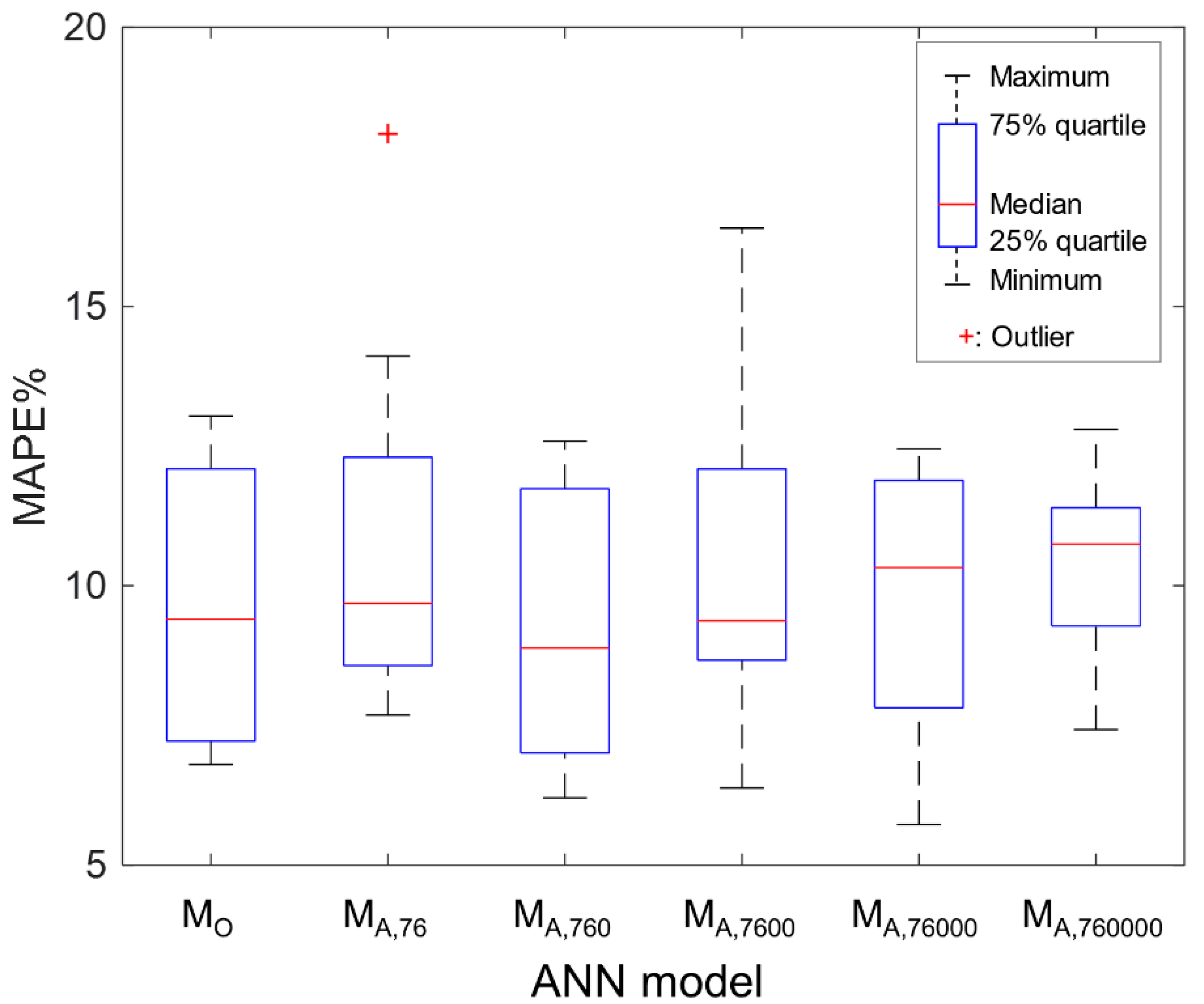
Figure 3 shows the comparison of the MAPE obtained in testing for different ANN models. All models use the same architecture (i.e., the size of layer and unit is the same for all models). However, each model was trained using a different training dataset, as shown in Table 2, and MAPE was computed in the testing phase. The procedure of obtaining the MAPE (for example, MA,760, shown in Figure 3) is as follows: (1) the architecture is trained using a training dataset of 760 points; (2) prediction is obtained using the test data of 8 points; (3) MAPE is computed; (4) step (1) to (3) is repeated 10 times. Maximum, minimum, 75% quartile, 25% quartile, and median of MAPE are presented in the boxplot. MAPE is a measure of the mean of the absolute error relative to the test datasets. MAPE scales the overall accuracy of the prediction through the entire domain. The lower the MAPE values, the higher the accuracy of the prediction. MA,760 showed the lowest median MAPE of 8.9% in ANN models using the augmented datasets. As the number of augmented data points increased, the median MAPE increased where larger augmented data points than M A,760 were used, as shown in MA,7600, MA,76000, and MA,760000. By comparing all MA,n models trained by using augmented datasets, it was found that the number of augmented data points influences the MAPE. It was also found that an investigation of the effect of the number of augmented points is required to minimize the MAPE. MO showed a median MAPE of 9.4%, which was larger than that of the MAPE of 8.9% for MA,760. By comparing MO with all MA,n models, it is found that the use of augmented datasets minimizes the MAPE more than that of MO. The augmentation achieved greater accuracy. In the present study, the augmented data set consisting of 760 points is considered sufficient to lower the MAPE in the testing.
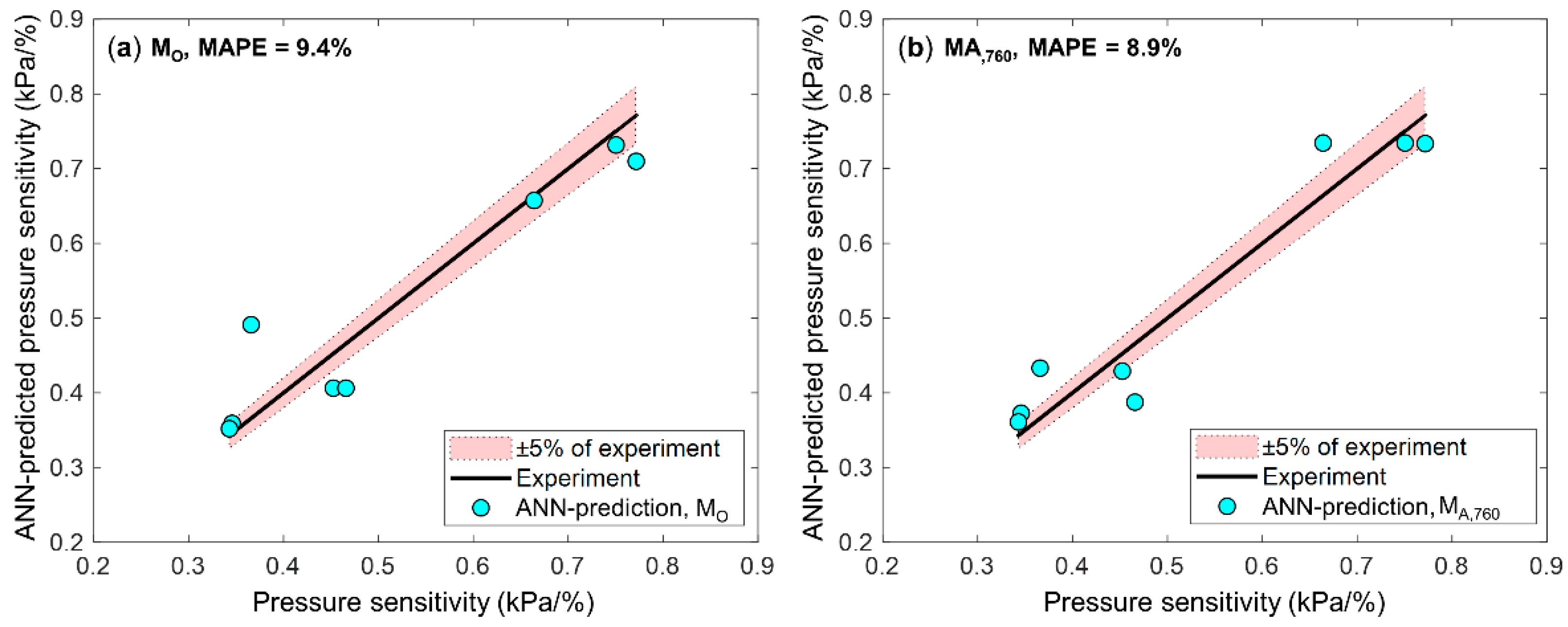
Figure 4 shows the accuracy of pressure sensitivity predicted by MO and MA,760 models when MAPE was the median of the MAPE values for those models. The confidence interval based on the experimental error of pressure sensitivity (i.e., ±5%) was selected as an interval to evaluate how precisely the ANN approximates the pressure sensitivity. By comparing the relative error of MO with MA, it was shown that four of eight test points were within 5% of the experimental measurement for both models. This indicates that both models predict the pressure sensitivity within ±5% of experimental measurement, while MA showed the more accurate and lower MAPE than MO, as shown in the comparison of the MAPE in the previous section.

6. Conclusions

Reducing time-consuming and expensive experiments is essential to enhancing PSP development. The present study investigated the application of an ANN to predict pressure sensitivity of the PSP to luminophore content and paint thickness with fewer than 102 data points. The ANN model was built and trained on the dataset produced by a data augmentation technique based on the experimental errors. It was concluded that the ANN model can obtain the correlation between pressure sensitivity with luminophore content and paint thickness in PSP development. The ANN model will reduce experimental costs. The ANN models trained by augmented datasets achieved 8.9% of MAPE in predicting pressure sensitivity. Augmented datasets have the potential to reduce MAPE with a small number of experimental data points.

Author Contributions

Conceptualization: H.S. and A.J.; methodology: D.K. and A.J.; validation: M.H. and D.K.; formal analysis: M.H. and D.K.; investigation: M.H., D.K. and Y.E.; resources: Y.E.; writing—original draft preparation: M.H. and D.K.; writing—review and editing: H.S., Y.E. and A.J.; supervision: H.S. and A.J. All authors have read and agreed to the published version of the manuscript.

Funding

This research received no external funding.

Institutional Review Board Statement

Not applicable.

Informed Consent Statement

Not applicable.

Data Availability Statement

The data presented in this study are available on request from the corresponding author, upon reasonable request.

Conflicts of Interest

The authors declare no conflict of interest.

Appendix A

This section presents the process of designing PSP where the experimental dataset was collected. Characterization of PSP was experimentally performed to design a PSP that increases pressure sensitivity as much as possible. A temperature/pressure-controlled chamber was used to place a PSP coupon under a controlled environment. Excitation and emission spectra of the PSP coupon were measured using a spectrometer. Luminescent intensity, temperature sensitivity, and pressure sensitivity (i.e., functions of PSP) were characterized. Luminophore concentration, luminophore content, paint thickness, and binder volume (i.e., components of PSP) were varied in order to identify a component that influences pressure sensitivity. To reduce experimental errors in the measurement caused by factors that vary from one measurement to another, the measurement was repeated multiple times.

Appendix B

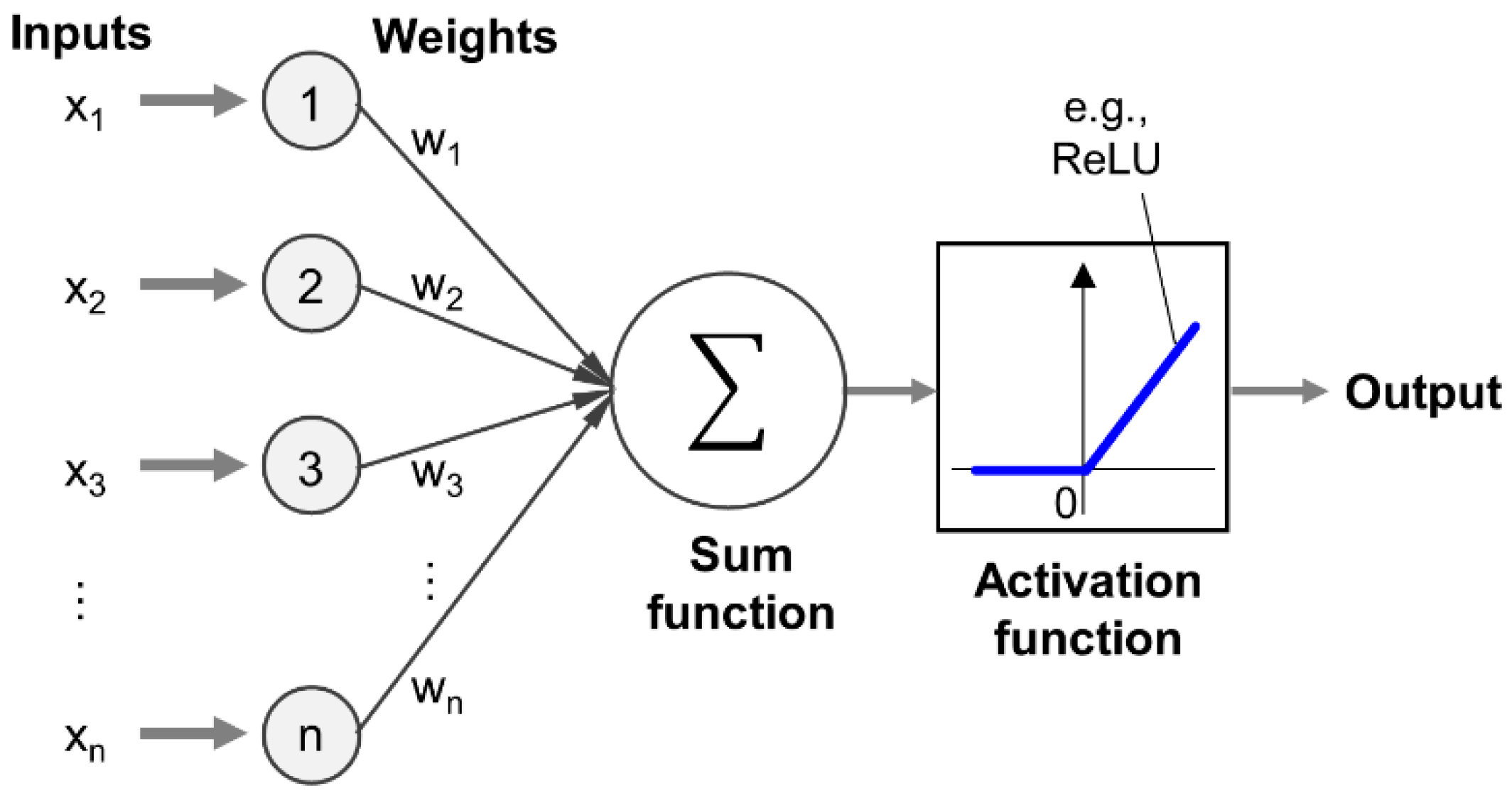
An ANN is a mathematical description of the nervous system’s structure in the human brain [43]. The simplest ANN (i.e., a simple perceptron) consists of an input layer and output layers of nodes. Those nodes are mutually fully connected. The perceptron is built in multiple layers consisting of multiple connected nodes. An output is produced through the ANN when a signal (i.e., data) is given to the input layer. The inside of the ANN contains weights to produce the desired output (i.e., prediction) corresponding to a given input. Figure A1 shows a simple ANN that consists of inputs, output, and inside the ANN, including weights, biases, a sum function, and activation function. Input is given from another system. The weight is a value that represents the influence of the previous layer’s input set or another processing element on this process element. The sum function calculates the net effects of inputs and weights on this process element (i.e., the weighted sum of nodes). The weighted sum contains a coefficient, w, as the weight, and a constant term called a bias. The activation function is used to determine the output value from the weighted sum and introduce a nonlinear effect into the output. The rectified linear unit (ReLU) is typically used as an activation function for nonlinear regression analysis [38].
Figure A1. Simple neural network. ReLU: rectified linear unit.
Sensors 21 05188 g0a1
Predictions using an ANN require training, as ANN architecture learns from the training dataset. By the back-propagation method [44], a constructed ANN architecture is trained to determine the weights and biases of the ANN that minimize the error between the ANN output (i.e., predicted values) and training dataset (i.e., observed values). A loss function is used to quantitatively evaluate the error. While various loss functions are available in ANN training, mean squared error (MSE) is commonly used to minimize the L2 norm of the error. The gradient descent method is used to find the weight and bias that minimize the error between the ANN output and training dataset [45]. The gradients of the loss function with respect to each weight and bias are calculated using the chain rule and partial derivatives. The gradients determine the updated directions of the weight and bias that reduce the loss function. The gradient descent method commonly used is Adam [39]. The weights are updated until the partial derivative of the loss function is zero during training. The amount that the weights are updated is called the learning rate. A larger learning rate yields faster convergence of the training; however, the training could be unstable. A lower learning rate stabilizes the training but requires a large number of iterations to converge. The trained ANN is used as an ANN model to make predictions based on a given input. The prediction performance of the ANN model is evaluated using metrics such as MSE, MAE, MAPE, R2, and RMSE, depending on the focus of the assessment. Further details on ANN are reviewed in references [26,46,47,48,49].
Construction of ANN architecture is required to develop an ANN model for prediction. A parametric study was preliminarily performed to determine the ANN architecture (i.e., size of units and layers) used in the present study. An ANN was constructed for different sizes of units and layers. The size of units and layers were varied to find a suitable ANN architecture that minimizes error between the prediction and training dataset, error’s bias, and error’s variance. ANN was trained using the Keras Regressor, an open-source ANN library, running with the TensorFlow, an open-source ANN library, under the Python environment, a programming language. The augmented dataset described in Section 2 was used for training. MSE was used as a loss function for training. MSE is calculated using the following equation:
MSE = 1 N i = 1 N ( o i p i ) 2 .
The variance of MSE was also assessed because a lower value of the MSE does not indicate that the precision in predictions is always better in the generalization that captures the dominant trend between inputs and outputs and fits the predictions within that trend [32].
ANN was trained using an augmented dataset of 100, 1000, and 10,000 entries. Table A1, Table A2 and Table A3 shows the MSE of the ANN for different sizes of layers and units. Table A4, Table A5 and Table A6 shows the variance of the MSE of the ANN for different sizes of layers and units. The size of hidden layers was varied from 1 to 5. The unit in the hidden layer was varied from 2, 4, 8, and 16. The criteria to determine ANN was as follows: (1) MSE is less than 0.1; (2) variance is as small as possible. The size of the hidden layer was determined to be 4, and the unit size was determined to be 4 based on the criteria.
Table A1. Mean squared error (MSE) of ANN for different layers and units in training for 100 entries of the augmented dataset.
LayerUnit = 2Unit = 4Unit = 8Unit = 16
10.4140.3040.1710.146
20.3900.1330.1070.031
30.5040.1450.0530.030
40.2660.1000.1030.013
50.1970.1780.0290.052
Table A2. MSE of ANN for different layers and units in training for 1000 entries of the augmented dataset.
LayerUnit = 2Unit = 4Unit = 8Unit = 16
10.4120.4120.1470.140
20.2900.1090.0570.038
30.5020.1830.0400.054
40.3060.0840.0520.032
50.1890.1570.0520.012
Table A3. MSE of ANN for different layers and units in training for 10,000 entries of the augmented dataset.
LayerUnit = 2Unit = 4Unit = 8Unit = 16
10.5030.1890.1880.132
20.3890.0940.0260.030
30.1770.1470.1470.011
40.1900.0710.0420.052
50.1900.0710.0430.028
Table A4. Variance of ANN for different layers and units in training for 100 entries of the augmented dataset.
LayerUnit = 2Unit = 4Unit = 8Unit = 16
10.5770.6830.8010.836
20.5900.8530.8740.947
30.4810.8340.9390.962
40.7340.8890.8760.963
50.7880.8030.9400.923
Table A5. Variance of ANN for different layers and units in training for 1000 entries of the augmented dataset.
LayerUnit = 2Unit = 4Unit = 8Unit = 16
10.5750.5750.8170.845
20.6960.8760.9320.956
30.4820.8020.9390.947
40.6820.8960.9360.958
50.7970.8280.9470.989
Table A6. Variance of ANN for different layers and units in training for 10,000 entries of the augmented dataset.
LayerUnit = 2Unit = 4Unit = 8Unit = 16
10.4840.7980.7970.841
20.5980.8860.9600.953
30.8120.8350.8380.988
40.7970.9090.9470.958
50.7980.9110.9290.975

References

  1. Sellers, M.E.; Nelson, M.A.; Roozeboom, N.H.; Burnside, N.J. Evaluation of unsteady pressure sensitive paint measurement technique for space launch vehicle buffet determination. In Proceedings of the AIAA SciTech Forum—55th AIAA Aerospace Sciences Meeting, Grapevine, TX, USA, 9–13 January 2017. [Google Scholar]
  2. Bitter, M.; Hara, T.; Hain, R.; Yorita, D.; Asai, K.; Kähler, C.J. Characterization of pressure dynamics in an axisymmetric separating/reattaching flow using fast-responding pressure-sensitive paint. Exp. Fluids 2012, 53, 1737–1749. [Google Scholar] [CrossRef] [Green Version]
  3. Running, C.L.; Sakaue, H.; Juliano, T.J. Hypersonic boundary-layer separation detection with pressure-sensitive paint for a cone at high angle of attack. Exp. Fluids 2019, 60, 23. [Google Scholar] [CrossRef]
  4. Quinn, M.K.; Kontis, K. Pressure-Sensitive Paint Measurements of Transient Shock Phenomena. Sensors 2013, 13, 4404–4427. [Google Scholar] [CrossRef] [PubMed] [Green Version]
  5. Lakowicz, J.R. Principles of Fluorescence Spectroscopy, 3rd ed.; Springer: Singapore, 2006. [Google Scholar] [CrossRef]
  6. Bell, J.H.; Schairer, E.T.; A Hand, L.; Mehta, R.D. Surface pressure measurements using luminescent coatings. Annu. Rev. Fluid Mech. 2001, 33, 155–206. [Google Scholar] [CrossRef]
  7. Kavandi, J.; Callis, J.; Gouterman, M.; Khalil, G.; Wright, D.; Green, E.; Burns, D.; McLachlan, B. Luminescent barometry in wind tunnels. Rev. Sci. Instrum. 1990, 61, 3340–3347. [Google Scholar] [CrossRef]
  8. Morris, M.; Benne, M.; Crites, R.; Donovan, J. Aerodynamic Measurements Based on Photoluminescence; American Institute of Aeronautics and Astronautics (AIAA): Reston, VA, USA, 1993. [Google Scholar]
  9. McLachlan, B.; Bell, J. Pressure-sensitive paint in aerodynamic testing. Exp. Therm. Fluid Sci. 1995, 10, 470–485. [Google Scholar] [CrossRef]
  10. Liu, T.; Campbell, B.T.; Burns, S.P.; Sullivan, J.P. Temperature- and pressure-sensitive luminescent paints in aerodynamics. Appl. Mech. Rev. 1997, 50, 227–246. [Google Scholar] [CrossRef]
  11. Liu, T.; Sullivan, J.P.; Asai, K.; Klein, C.; Egami, Y. Pressure and Temperature Sensitive Paints, 2nd ed.; Springer International Publishing: Berlin/Heidelberg, Germany, 2021; ISBN 978-3-030-68055-8. [Google Scholar]
  12. Sakaue, H.; Ishii, K. Optimization of anodized-aluminum pressure-sensitive paint by controlling luminophore concentration. Sensors 2010, 10, 6836–6847. [Google Scholar] [CrossRef]
  13. Grenoble, S.; Gouterman, M.; Khalil, G.; Callis, J.; Dalton, L. Pressure-sensitive paint (PSP): Concentration quenching of platinum and magnesium porphyrin dyes in polymeric films. J. Lumin. 2005, 113, 33–44. [Google Scholar] [CrossRef]
  14. Hayashi, T.; Sakaue, H. Dynamic and steady characteristics of polymer-ceramic pressure-sensitive paint with variation in layer thickness. Sensors 2017, 17, 1125. [Google Scholar] [CrossRef] [Green Version]
  15. Gregory, J.; Asai, K.; Kameda, M.; Liu, T.; Sullivan, J.P. A review of pressure-sensitive paint for high-speed and unsteady aerodynamics. Proc. Inst. Mech. Eng. Part G J. Aerosp. Eng. 2008, 222, 249–290. [Google Scholar] [CrossRef]
  16. Sakaue, H.; Ishii, K. A dipping duration study for optimization of anodized-aluminum pressure-sensitive paint. Sensors 2010, 10, 9799–9807. [Google Scholar] [CrossRef] [Green Version]
  17. Quinn, M.K.; Yang, L.; Kontis, K. Pressure-sensitive paint: Effect of substrate. Sensors 2011, 11, 11649–11663. [Google Scholar] [CrossRef] [Green Version]
  18. Yeh, I.-C. Modeling of strength of high-performance concrete using artificial neural networks. Cem. Concr. Res. 1998, 28, 1797–1808. [Google Scholar] [CrossRef]
  19. Schmidt, J.; Marques, M.R.G.; Botti, S.; Marques, M.A.L. Recent advances and applications of machine learning in solid-state materials science. NPJ Comput. Mater. 2019, 5, 1–36. [Google Scholar] [CrossRef]
  20. Tasoujian, S.; Salavati, S.; Franchek, M.A.; Grigoriadis, K.M. Robust delay-dependent LPV synthesis for blood pressure control with real-time Bayesian parameter estimation. IET Control. Theory Appl. 2020, 14, 1334–1345. [Google Scholar] [CrossRef]
  21. Yamamoto, K.; Togami, T.; Yamaguchi, N.; Ninomiya, S. Machine learning-based calibration of low-cost air temperature sensors using environmental data. Sensors 2017, 17, 1290. [Google Scholar] [CrossRef] [PubMed] [Green Version]
  22. Wang, Y.; Dou, Y.; Yang, W.; Guo, J.; Chang, X.; Ding, M.; Tang, X. A new machine learning algorithm for numerical prediction of near-Earth environment sensors along the inland of East Antarctica. Sensors 2021, 21, 755. [Google Scholar] [CrossRef] [PubMed]
  23. Moaveni, B.; Fathabadi, F.R.; Molavi, A. Supervisory predictive control for wheel slip prevention and tracking of desired speed profile in electric trains. ISA Trans. 2020, 101, 102–115. [Google Scholar] [CrossRef] [PubMed]
  24. Karimi, M.; Jahanshahi, A.; Mazloumi, A.; Sabzi, H.Z. Border gateway protocol anomaly detection using neural network. Proc. IEEE Int. Conf. Big Data 2019, 6092–6094. [Google Scholar] [CrossRef]
  25. Kim, D.; Kim, B. Application of neural network and FEM for metal forming processes. Int. J. Mach. Tools Manuf. 2000, 40, 911–925. [Google Scholar] [CrossRef]
  26. Liakos, K.G.; Busato, P.; Moshou, D.; Pearson, S.; Bochtis, D. Machine learning in agriculture: A review. Sensors 2018, 18, 2674. [Google Scholar] [CrossRef] [PubMed] [Green Version]
  27. Ward, L.; O’Keeffe, S.C.; Stevick, J.; Jelbert, G.R.; Aykol, M.; Wolverton, C. A machine learning approach for engineering bulk metallic glass alloys. Acta Mater. 2018, 159, 102–111. [Google Scholar] [CrossRef]
  28. Feng, S.; Zhou, H.; Dong, H. Using deep neural network with small dataset to predict material defects. Mater. Des. 2019, 162, 300–310. [Google Scholar] [CrossRef]
  29. Roshani, M.; Phan, G.T.; Ali, P.J.M.; Roshani, G.H.; Hanus, R.; Duong, T.; Corniani, E.; Nazemi, E.; Kalmoun, E.M. Evaluation of flow pattern recognition and void fraction measurement in two phase flow independent of oil pipeline’s scale layer thickness. Alex. Eng. J. 2021, 60, 1955–1966. [Google Scholar] [CrossRef]
  30. Voghoei, S.; Tonekaboni, N.H.; Yazdansepas, D.; Soleymani, S.; Farahani, A.; Arabnia, H.R. Personalized feedback emails. In Proceedings of the ACM SE ‘20: 2020 ACM Southeast Conference, Tampa, FL, USA, 2–4 April 2020; pp. 18–25. [Google Scholar] [CrossRef]
  31. Arabi, M.; Beheshtitabar, E.; Ghadirifaraz, B.; Forjanizadeh, B. Optimum locations for intercity bus terminals with the AHP approach—Case study of the city of Esfahan. Int. J. Environ. Ecol. Eng. 2015, 9, 545–551. [Google Scholar] [CrossRef]
  32. Mehta, P.; Bukov, M.; Wang, C.H.; Day, A.G.R.; Richardson, C.; Fisher, C.K.; Schwab, D.J. A high-bias, low-variance in-troduction to machine learning for physicists. Phys. Rep. 2019, 810, 1–124. [Google Scholar] [CrossRef] [PubMed]
  33. Cawley, G.C.; Talbot, N.L.C. On over-fitting in model selection and subsequent selection bias in performance evaluation. J. Mach. Learn. Res. 2010, 11, 2079–2107. [Google Scholar]
  34. Halevy, A.; Norvig, P.; Pereira, F. The unreasonable effectiveness of data. IEEE Intell. Syst. 2009, 24, 8–12. [Google Scholar] [CrossRef]
  35. Chen, X.; Xu, Y.; Kee Wong, D.W.; Wong, T.Y.; Liu, J. Glaucoma detection based on deep convolutional neural network. In Proceedings of the Annual International Conference of the IEEE Engineering in Medicine and Biology Society, EMBS, Milan, Italy, 25–29 August 2015; Volume 2015, pp. 715–718. [Google Scholar]
  36. Van Dyk, D.; Meng, X.-L. The art of data augmentation. J. Comput. Graph. Stat. 2001, 10, 1–50. [Google Scholar] [CrossRef]
  37. Zhao, W.; Bhushan, A.; Santamaria, A.; Simon, M.G.; Davis, C.E. Machine learning: A crucial tool for sensor design. Algorithms 2008, 1, 130–152. [Google Scholar] [CrossRef] [Green Version]
  38. Glorot, X.; Bordes, A.; Bengio, Y. Deep sparse rectifier neural networks. In Proceedings of the Fourteenth International Conference on Artificial Intelligence and Statistics, Fort Lauderdale, FL, USA, 11–13 April 2011. [Google Scholar]
  39. Kingma, D.P.; Ba, J. Adam: A method for stochastic optimization. In Proceedings of the 3rd International Conference on Learning Representations, ICLR, San Diego, CA, USA, 5–8 May 2015. [Google Scholar]
  40. De Myttenaere, A.; Golden, B.; le Grand, B.; Rossi, F. Mean absolute percentage error for regression models. Neurocomputing 2016, 192, 38–48. [Google Scholar] [CrossRef] [Green Version]
  41. Gupta, H.; Kling, H.; Yilmaz, K.K.; Martinez, G.F. Decomposition of the mean squared error and NSE performance criteria: Implications for improving hydrological modelling. J. Hydrol. 2009, 377, 80–91. [Google Scholar] [CrossRef] [Green Version]
  42. Blondel, V.D.; Guillaume, J.-L.; Lambiotte, R.; Lefebvre, E. Fast unfolding of communities in large networks. J. Stat. Mech. Theory Exp. 2008, 2008, P10008. [Google Scholar] [CrossRef] [Green Version]
  43. Amit, D.J. Modeling Brain Function; Cambridge University Press: Cambridge, UK, 1989. [Google Scholar]
  44. Rumelhart, D.E.; Hinton, G.E.; Williams, R.J. Learning representations by back-propagating errors. Nature 1986, 323, 533–536. [Google Scholar] [CrossRef]
  45. Bottou, L. Large-scale machine learning with stochastic gradient descent. In Proceedings of the COMPSTAT 2010—19th International Conference on Computational Statistics, Paris, France, 22–27 August 2010; pp. 177–186. [Google Scholar] [CrossRef] [Green Version]
  46. Yildiz, B.; Bilbao, J.; Sproul, A. A review and analysis of regression and machine learning models on commercial building electricity load forecasting. Renew. Sustain. Energy Rev. 2017, 73, 1104–1122. [Google Scholar] [CrossRef]
  47. Dreiseitl, S.; Ohno-Machado, L. Logistic regression and artificial neural network classification models: A methodology review. J. Biomed. Inform. 2002, 35, 352–359. [Google Scholar] [CrossRef] [Green Version]
  48. Dasgupta, A.; Sun, Y.V.; König, I.; Bailey-Wilson, J.; Malley, J.D. Brief review of regression-based and machine learning methods in genetic epidemiology: The Genetic Analysis Workshop 17 experience. Genet. Epidemiol. 2011, 35, S5–S11. [Google Scholar] [CrossRef] [Green Version]
  49. Christodoulou, E.; Ma, J.; Collins, G.S.; Steyerberg, E.W.; Verbakel, J.Y.; van Calster, B. A systematic review shows no performance benefit of machine learning over logistic regression for clinical prediction models. J. Clin. Epidemiol. 2019, 110, 12–22. [Google Scholar] [CrossRef] [PubMed]
Figure 1. (a) Schematic concept of data augmentation by newly produced data points (augmented data points) from experimental data points using confidence intervals based on the experimental errors. (b) An example of data augmentation: 100 augmented data points, DA,7600, were created around each experimental data point, and a total of 76 × 100 was produced as output for pressure sensitivity for different paint thicknesses and luminophore contents as inputs.
Sensors 21 05188 g001
Figure 2. Architecture and corresponding dataset of the artificial neural network (ANN) model for predicting pressure sensitivity to luminophore content and paint thickness.
Sensors 21 05188 g002
Figure 3. Comparison of mean absolute percentage error (MAPE) for different ANN models. Training and testing were repeated 10 times for each ANN model. The figure indicates that MA,760 has the lowest MAPE.
Sensors 21 05188 g003
Figure 4. Prediction accuracy of MO and MA,760 models for the test dataset. The shaded area enclosed with a dashed line indicates the confidence interval of ±5% of the experimental measurement. (a) The model MO, trained by DO,76. Four of eight test points were within 5% of the experimental measurement and MAPE was 9.4%. (b) The model MA,760, trained by augmented dataset, DA,760. Four of eight test points were within 5% of the experimental measurement and MAPE was 8.9%. The figure indicates that both models predict the pressure sensitivity within ±5% of the experimental measurement.
Sensors 21 05188 g004
Table 1. Range and experimental errors of experimental dataset for pressure-sensitive paint (PSP) coupons.
ComponentMinimumMaximumRelative Error
Paint Thickness (µm)4.53267.635±9% of paint thickness
Luminophore Content (mg)3.0 × 10−82.0 × 10−5±7% of luminophore content
Pressure Sensitivity (%/kPa)0.28730.8094±5% of pressure sensitivity
Table 2. ANN models. DO,n represents an experimental dataset and DA,n represents an augmented dataset. n is the number of data points.
ANN ModelTraining DatasetTest Dataset
MA,76DA,76DO,8
MA,760DA,760DO,8
MA,7600DA,7600DO,8
MA,76000DA,76000DO,8
MA,760000DA,760000DO,8
MODO,76DO,8
Publisher’s Note: MDPI stays neutral with regard to jurisdictional claims in published maps and institutional affiliations.