
Towards an Optimal Footprint Based Area Coverage Strategy for a False-Ceiling Inspection Robot

 ,
,  , , and
Abstract
:1. Introduction
2. Objectives
- A zig-zag area coverage strategy is proposed for false-ceiling inspection, where the area coverage is defined in terms of the robot footprint, which is dependent on the position and orientation of the camera (camera installation parameters).
- Formulate cost functions based on area missed and path-length covered during the inspection by the robot.
- Estimate the functional footprint by finding the optimal values for camera installation parameters by minimizing the costs using multi-objective optimization.
- Validate the results of the Raptor robot by conducting experiment trials on a false ceiling test-bed.
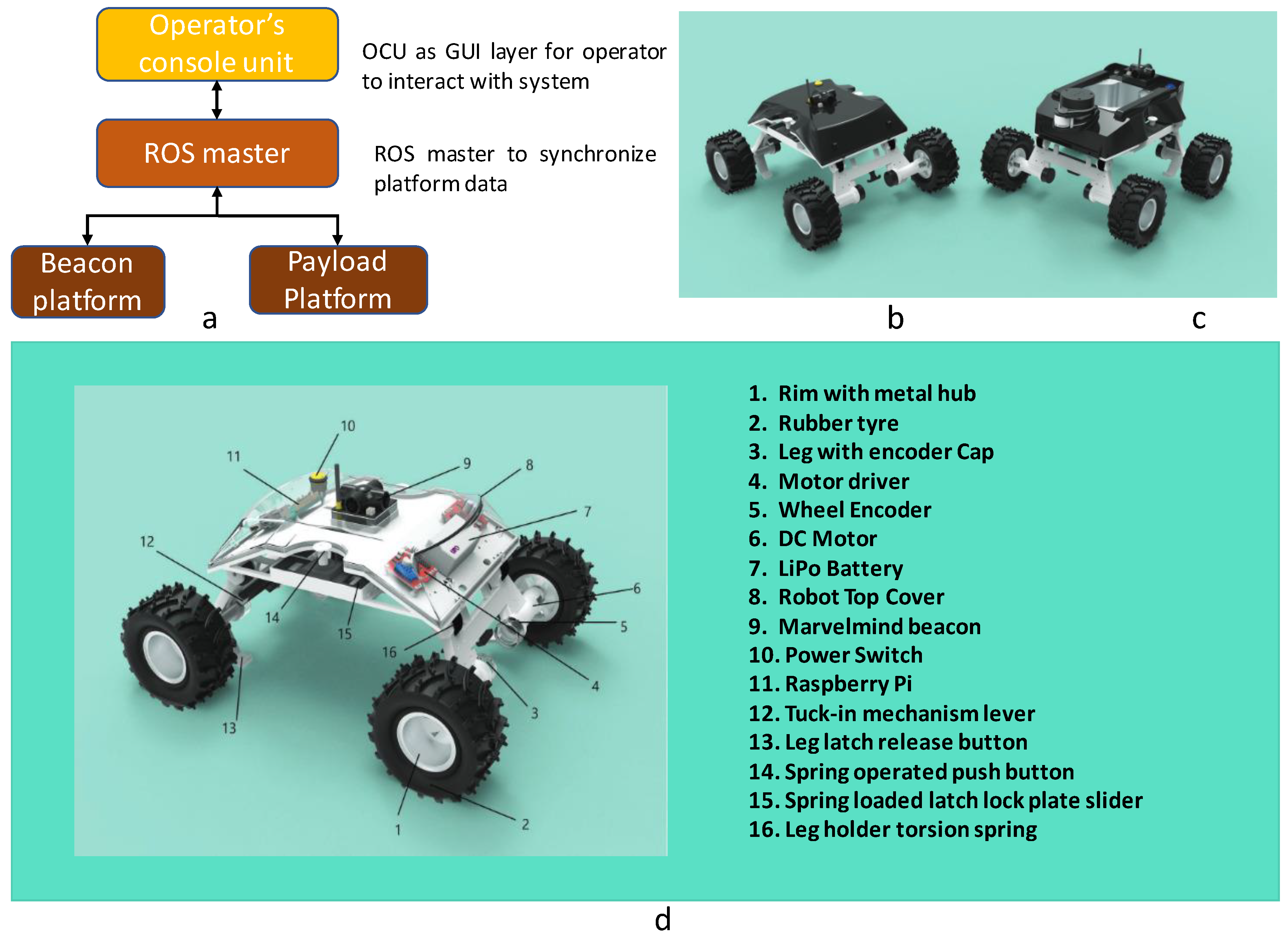
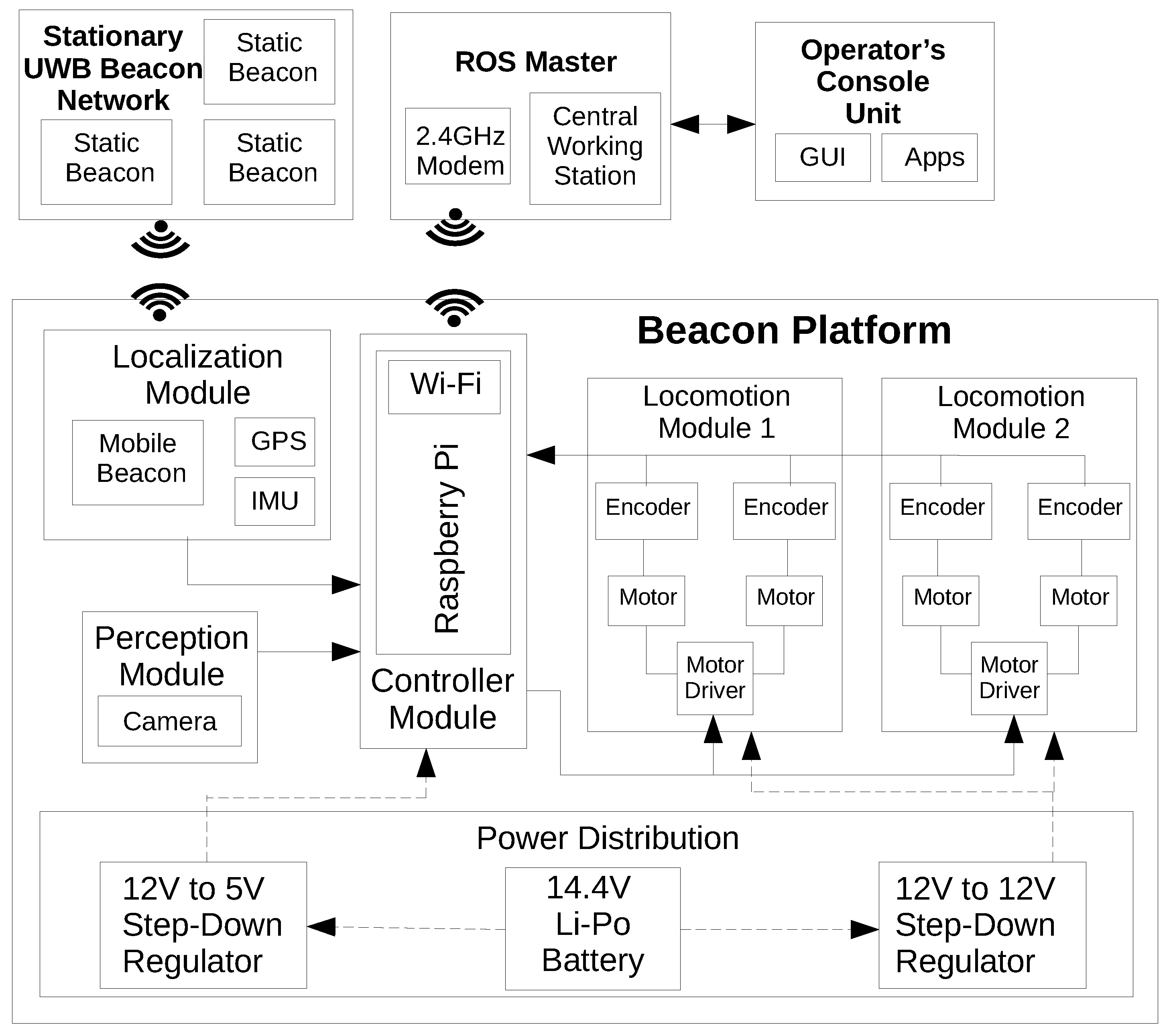
3. System Architecture
Control and Autonomy
4. Path-Planning Strategy
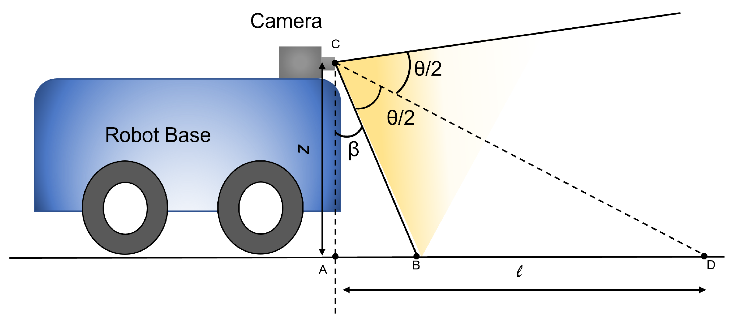
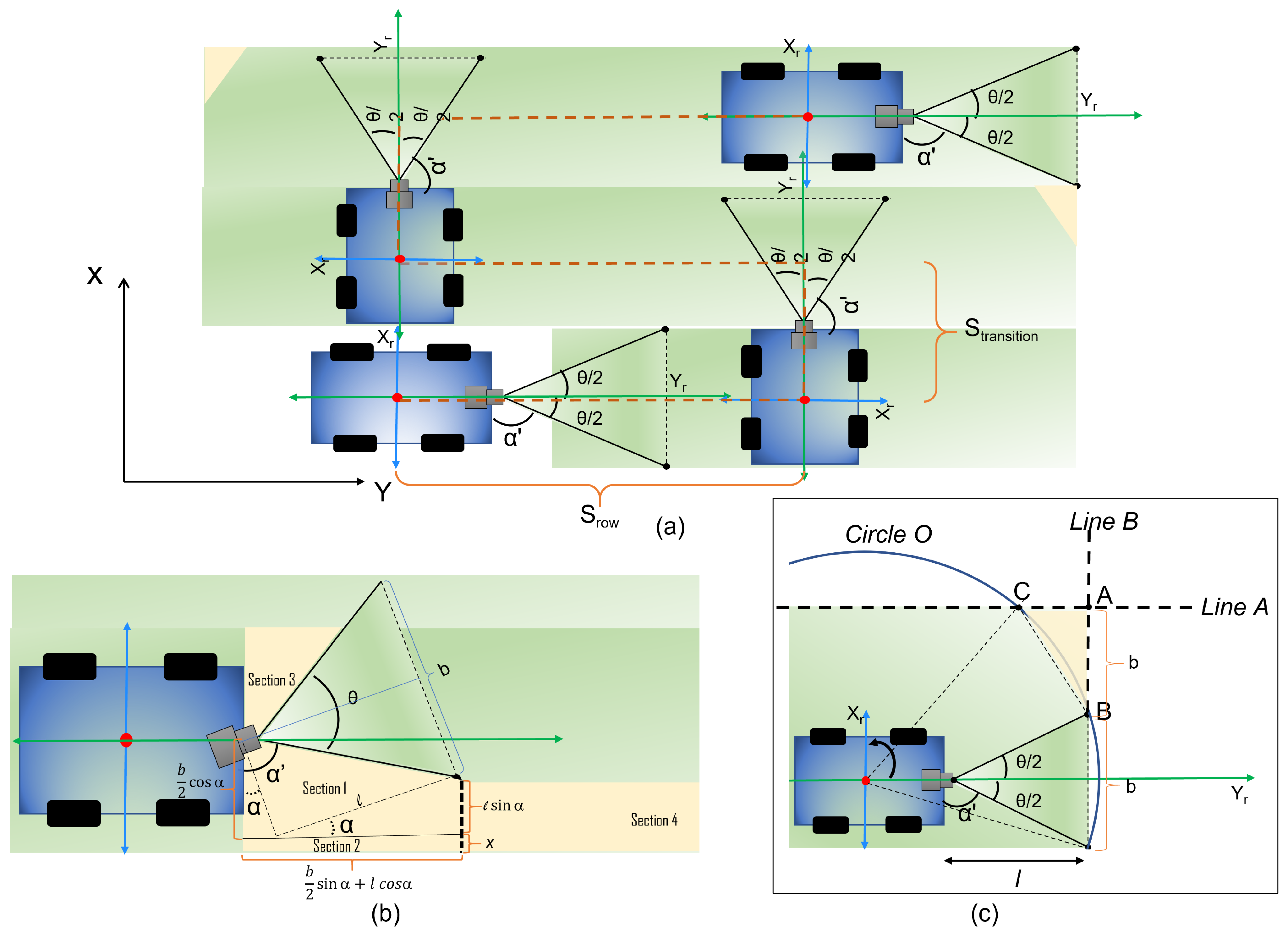
4.1. Robot Footprint Definition
- Position of camera mounting in both the x and y-axis.
- The horizontal mounting angle (yaw angle).
- The vertical mounting angle (pitch angle).
4.2. Zig-Zag Based Area Coverage
5. Optimal Coverage Strategy
5.1. Total Zig-Zag Path Length Computation
5.2. Total Area Missed
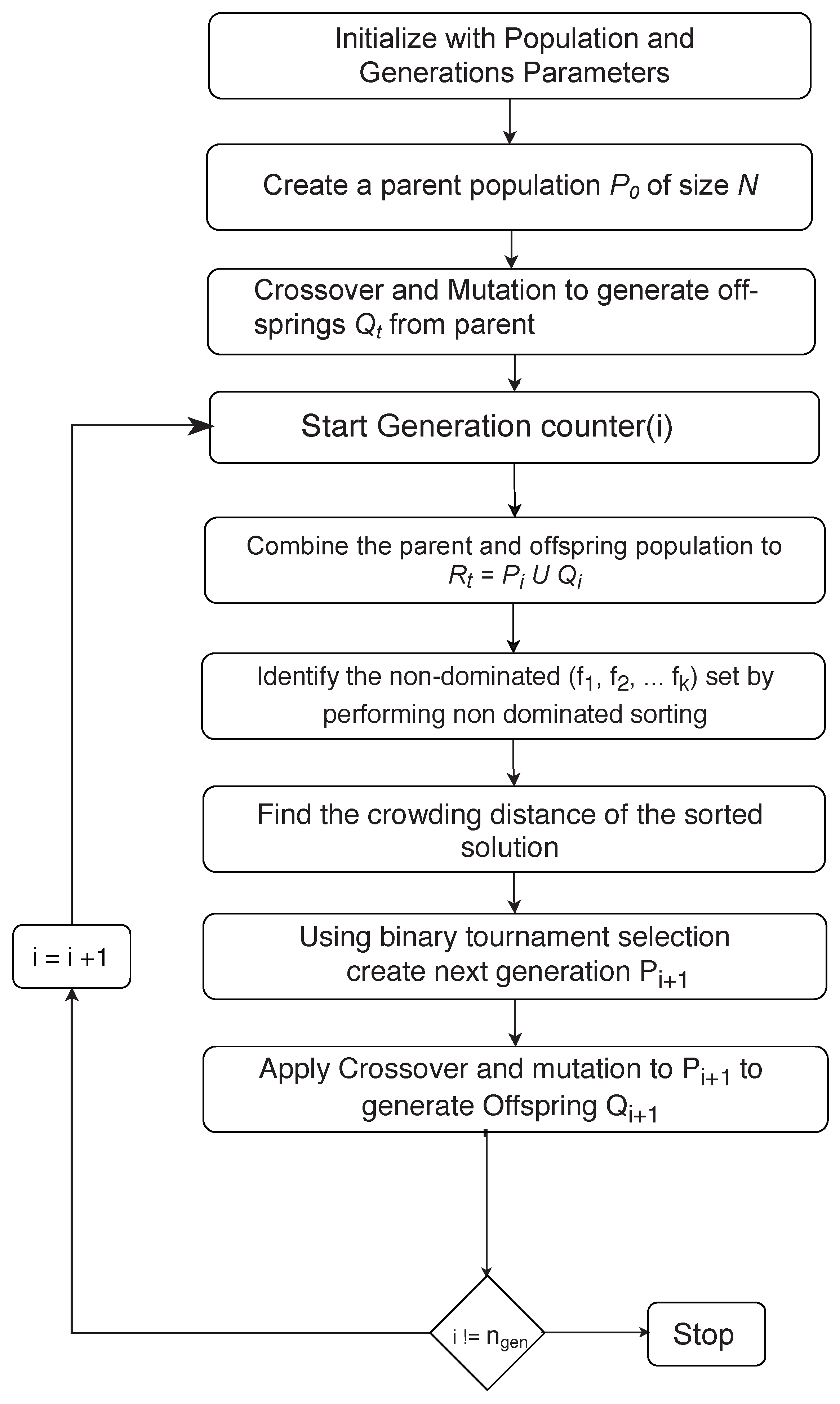
5.2.1. NSGA-2
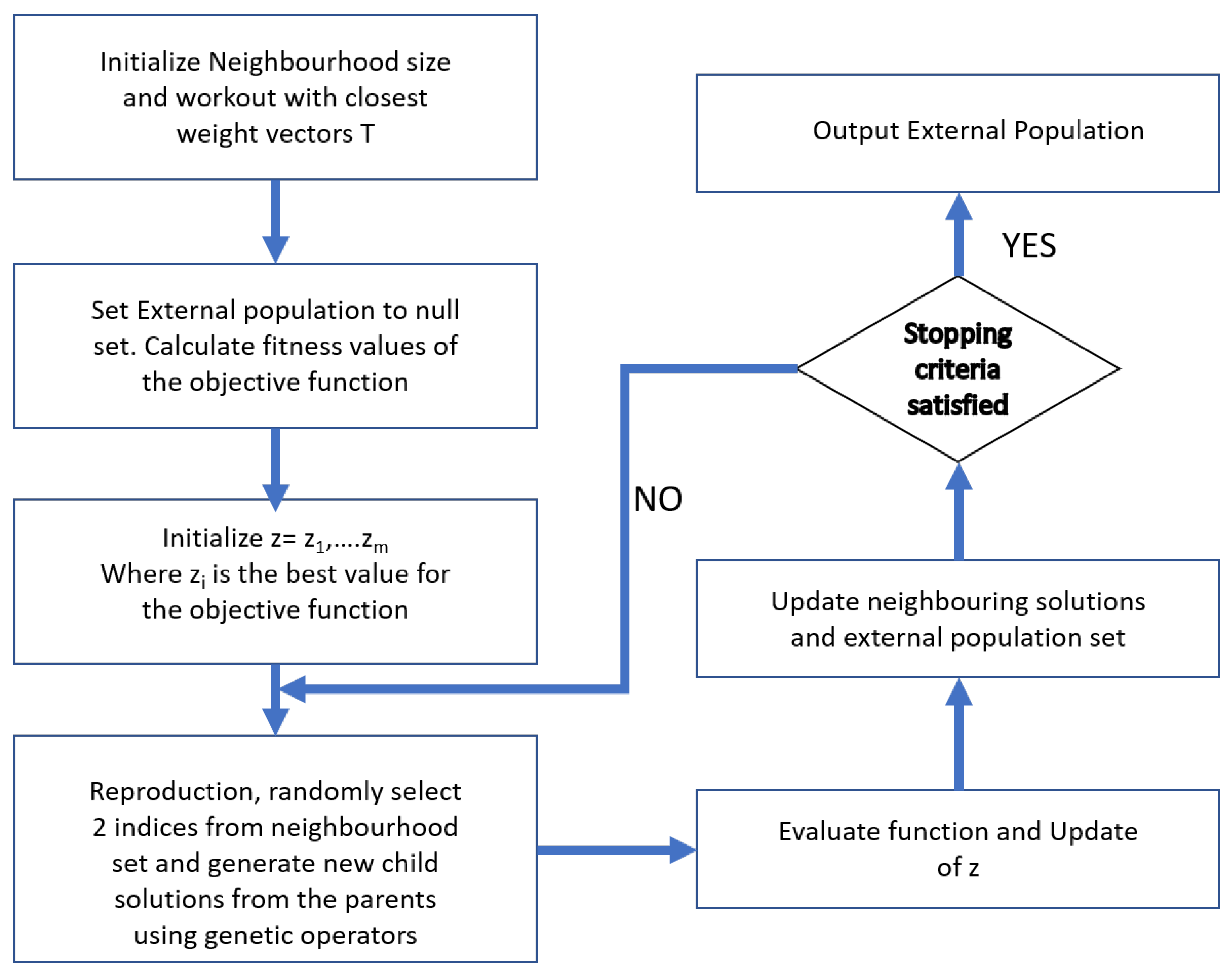
5.2.2. MOEA/D
6. Results and Discussion
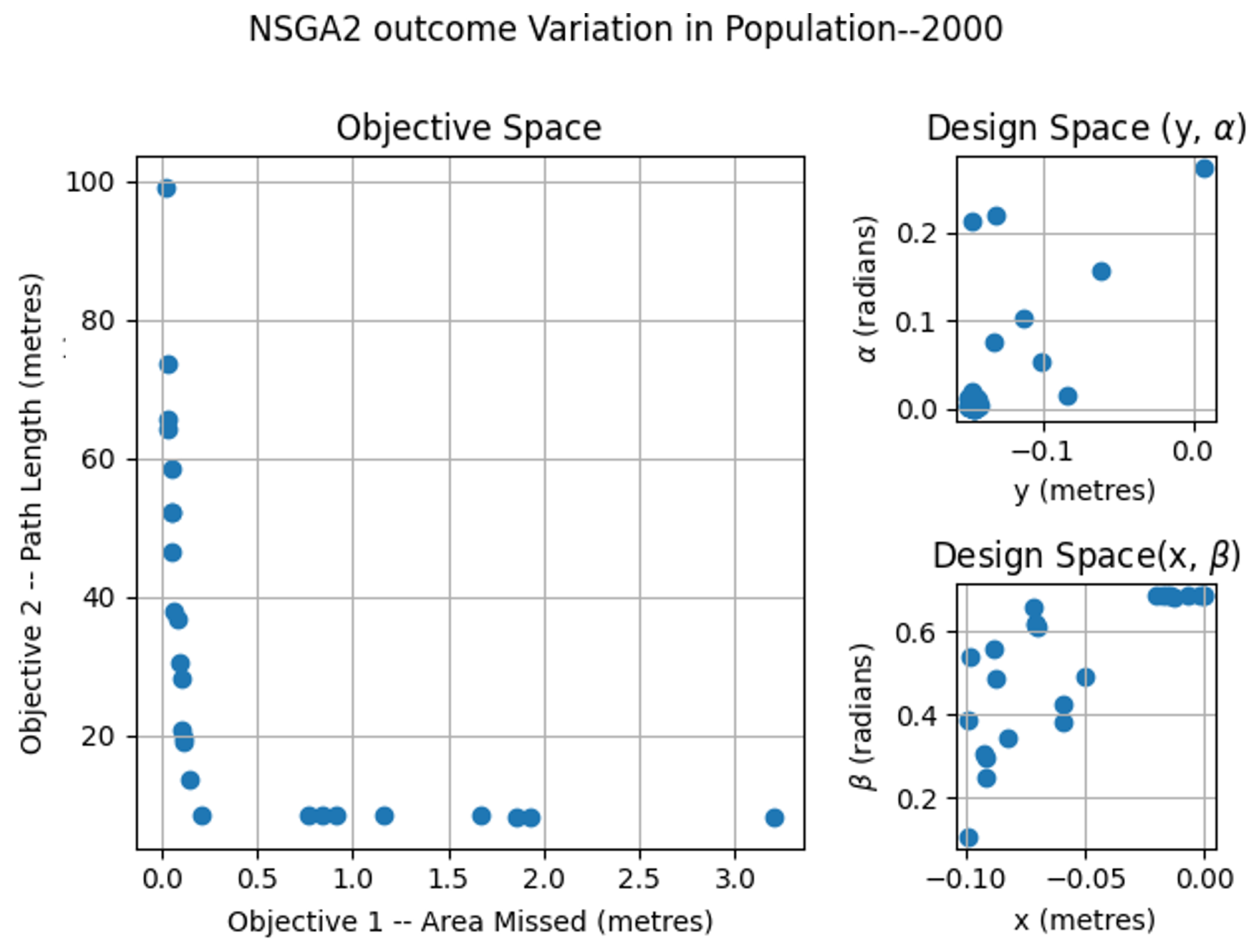
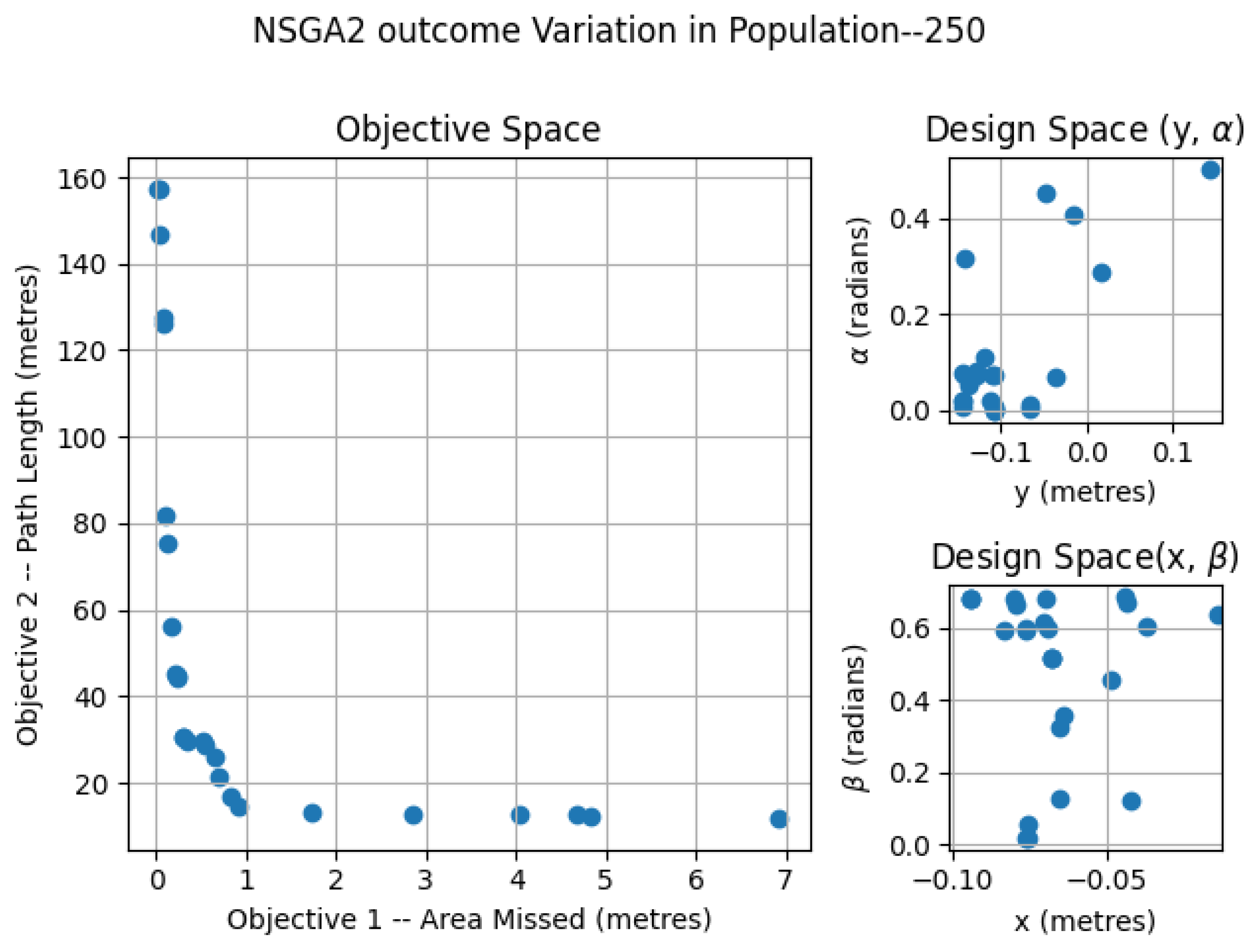
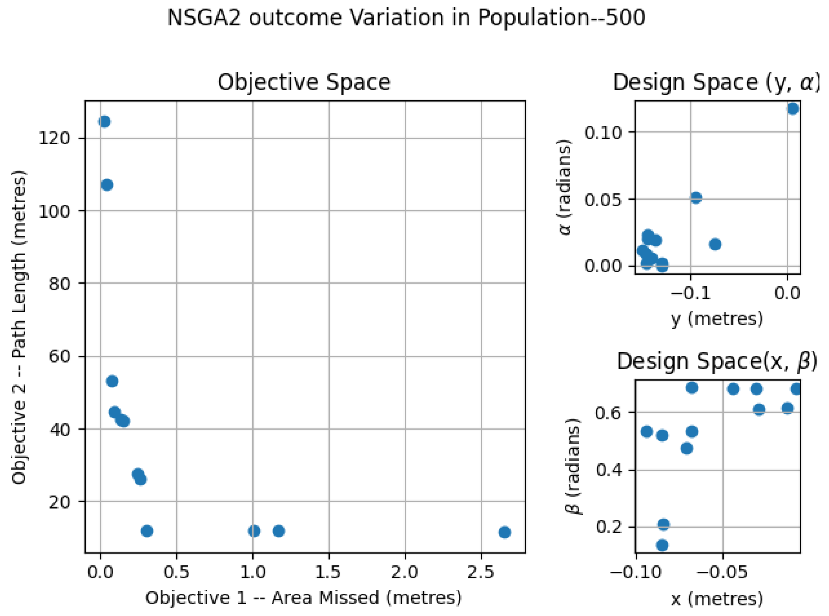
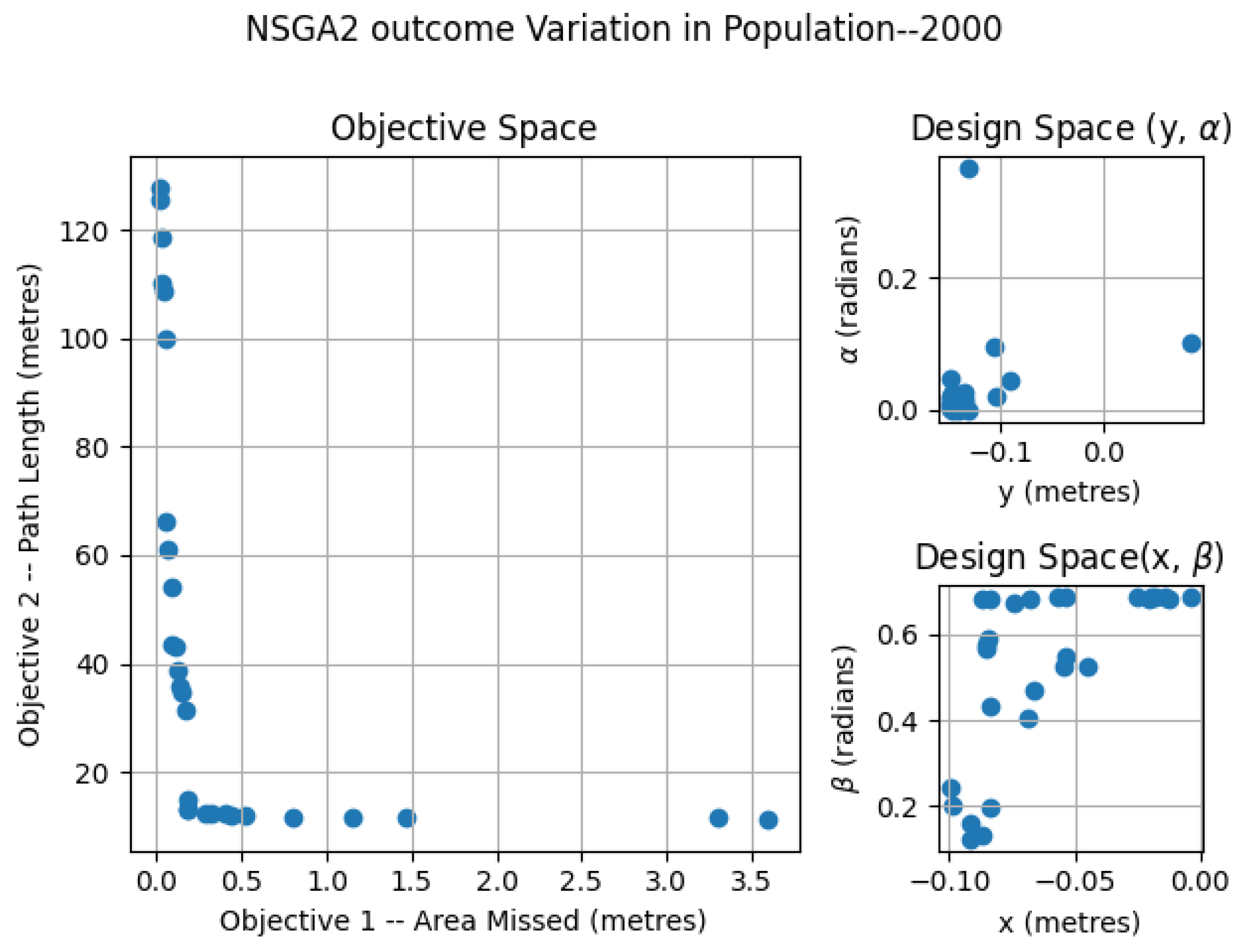
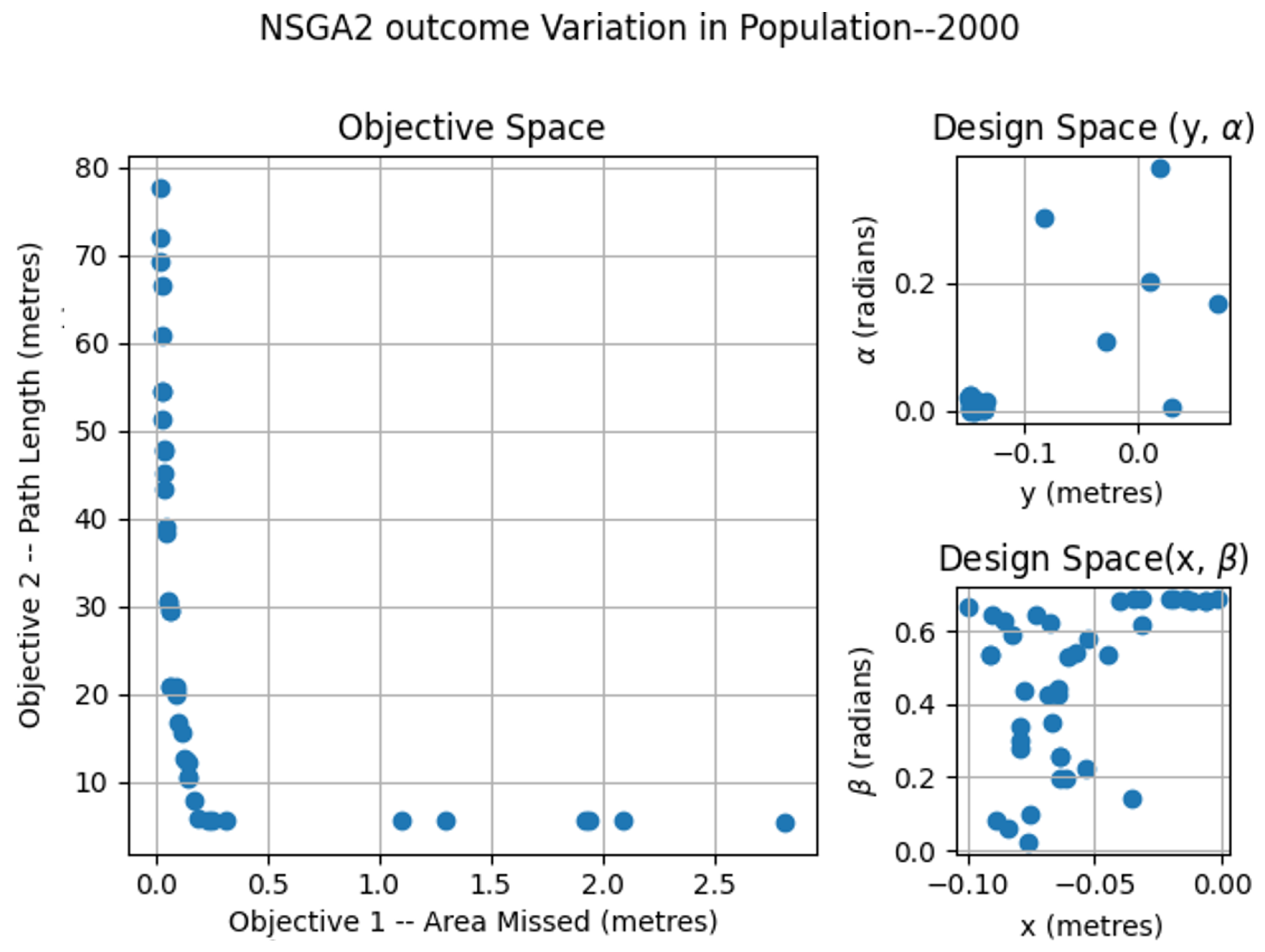
6.1. NSGA2—Variation of Population
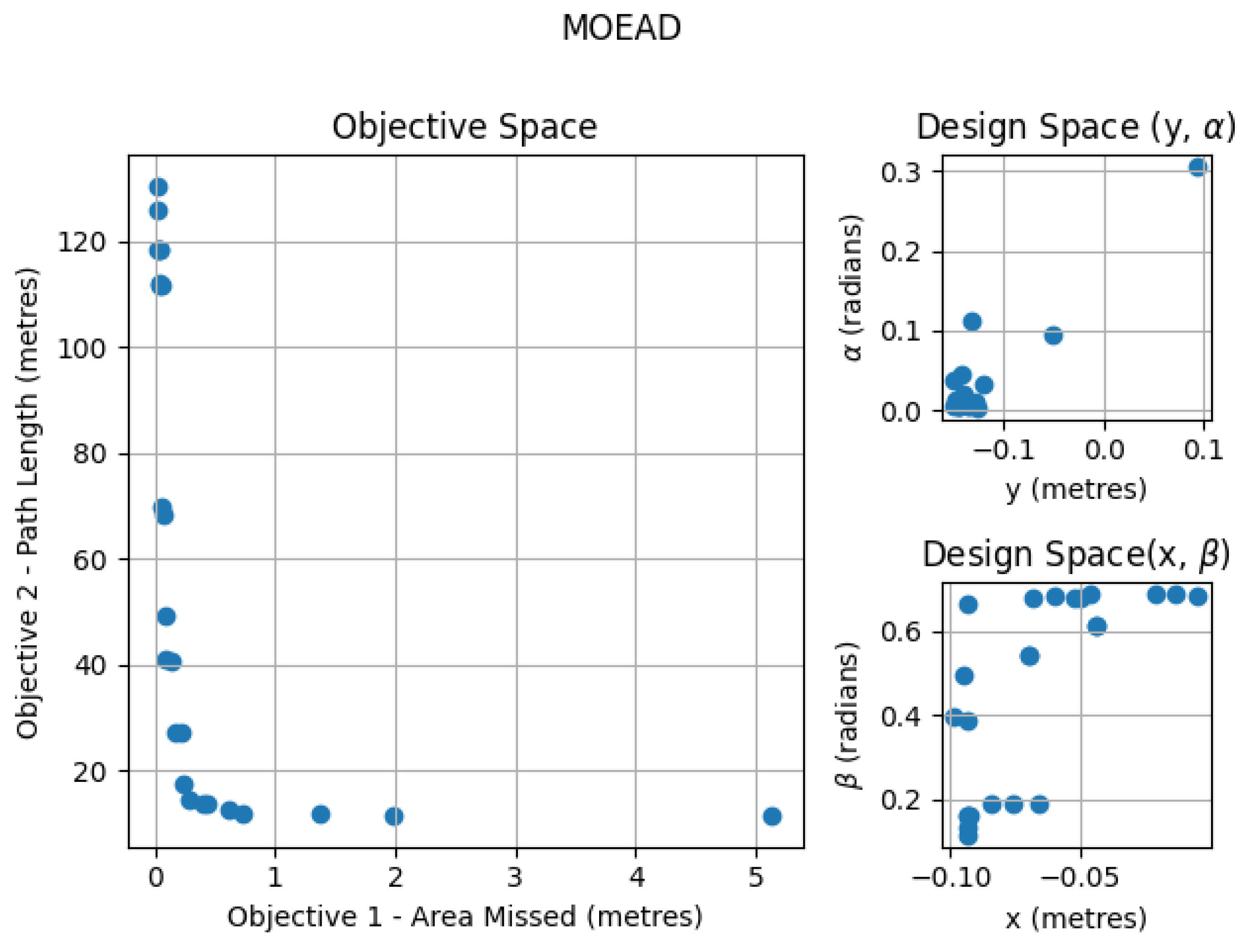
6.2. MOEA/D
6.3. NSGA-2 Variation of Area
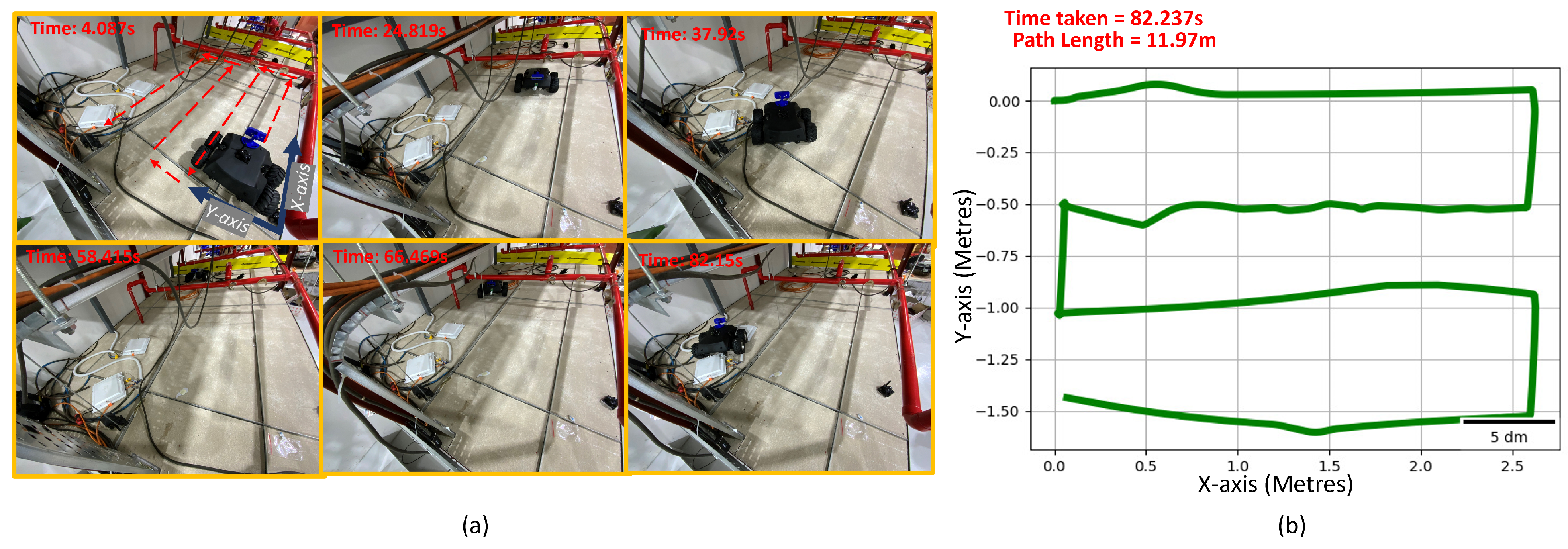
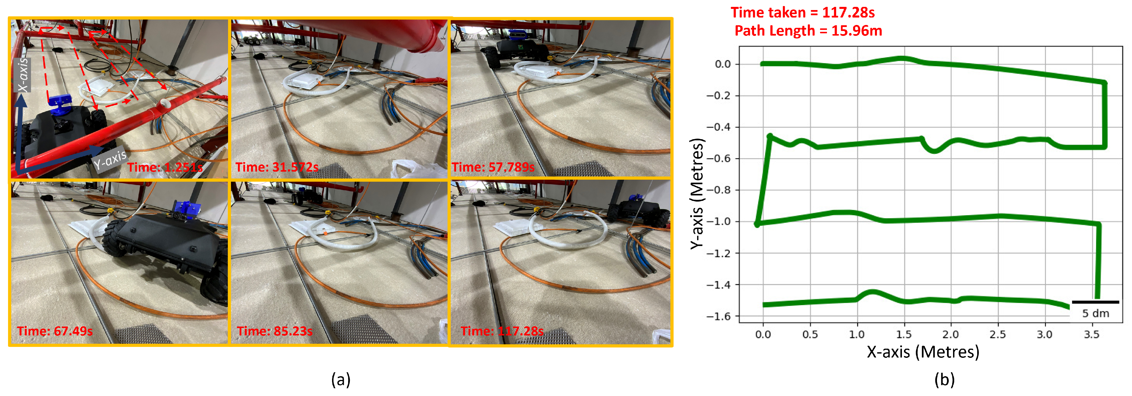
6.4. Experiments
7. Conclusions and Future Works
Author Contributions
Funding
Institutional Review Board Statement
Informed Consent Statement
Data Availability Statement
Conflicts of Interest
References
- Pest Control Market by Pest Type. Available online: https://www.marketsandmarkets.com/Market-Reports/pest-control-market-144665518.html (accessed on 2 June 2021).
- QUINCE Market Insights. Available online: https://www.globenewswire.com/news-release/2021/05/24/2234537/0/en/Global-Pest-Control-Market-is-Estimated-to-Grow-at-a-CAGR-of-5-25-from-2021-to-2030.html (accessed on 2 June 2021).
- Rabiee, M.H.; Mahmoudi, A.; Siahsarvie, R.; Kryštufek, B.; Mostafavi, E. Rodent-borne diseases and their public health importance in Iran. PLoS Negl. Trop. Dis. 2018, 12, e0006256. [Google Scholar] [CrossRef] [Green Version]
- Nimo-Paintsil, S.C.; Fichet-Calvet, E.; Borremans, B.; Letizia, A.G.; Mohareb, E.; Bonney, J.H.; Obiri-Danso, K.; Ampofo, W.K.; Schoepp, R.J.; Kronmann, K.C. Rodent-borne infections in rural Ghanaian farming communities. PLoS ONE 2019, 14, e0215224. [Google Scholar] [CrossRef] [PubMed]
- Meerburg, B.G.; Singleton, G.R.; Kijlstra, A. Rodent-borne diseases and their risks for public health. Crit. Rev. Microbiol. 2009, 35, 221–270. [Google Scholar] [CrossRef] [PubMed]
- Costa, F.; Ribeiro, G.S.; Felzemburgh, R.D.; Santos, N.; Reis, R.B.; Santos, A.C.; Fraga, D.B.M.; Araujo, W.N.; Santana, C.; Childs, J.E.; et al. Influence of household rat infestation on Leptospira transmission in the urban slum environment. PLoS Negl. Trop. Dis. 2014, 8, e3338. [Google Scholar] [CrossRef] [PubMed] [Green Version]
- Tapsoba, C. Rodents Damage Cable, Causing Internet Failure. Available online: http://www.northwesttalon.org/2017/03/03/rodents-damage-cable-causing-internet-failure/ (accessed on 21 June 2016).
- Almeida, A.; Corrigan, R.; Sarno, R. The economic impact of commensal rodents on small businesses in Manhattan’s Chinatown: Trends and possible causes. Suburb. Sustain. 2013, 1, 2. [Google Scholar] [CrossRef]
- Jassat, W.; Naicker, N.; Naidoo, S.; Mathee, A. Rodent control in urban communities in Johannesburg, South Africa: From research to action. Int. J. Environ. Health Res. 2013, 23, 474–483. [Google Scholar] [CrossRef]
- Kariduraganavar, R.M.; Yadav, S.S. Design and Implementation of IoT Based Rodent Monitoring and Avoidance System in Agricultural Storage Bins. In Emerging Trends in Photonics, Signal Processing and Communication Engineering; Springer: Berlin/Heidelberg, Germany, 2020; pp. 233–241. [Google Scholar]
- Ross, R.; Parsons, L.; Thai, B.S.; Hall, R.; Kaushik, M. An IOT smart rodent bait station system utilizing computer vision. Sensors 2020, 20, 4670. [Google Scholar] [CrossRef]
- Parsons, L.; Ross, R. A computer-vision approach to bait level estimation in rodent bait stations. Comput. Electron. Agric. 2020, 172, 105340. [Google Scholar] [CrossRef]
- Sowmika, T.; Malathi, G. IOT Based Smart Rodent Detection and Fire Alert System in Farmland. Int. Res. J. Multidiscip. Technovation 2020, 1–6. [Google Scholar] [CrossRef]
- Cambra, C.; Sendra, S.; Garcia, L.; Lloret, J. Low cost wireless sensor network for rodents detection. In Proceedings of the 2017 10th IFIP Wireless and Mobile Networking Conference (WMNC), Valencia, Spain, 25–27 September 2017; pp. 1–7. [Google Scholar]
- Walsh, J.R.; Lynch, P.J. Remote Sensing Rodent Bait Station Tray. U.S. Patent 10,897,887, 26 January 2021. [Google Scholar]
- Barnett, S. Exploring, sampling, neophobia, and feeding. In Rodent Pest Management; CRC Press: Boca Raton, FL, USA, 2018; pp. 295–320. [Google Scholar]
- Feng, A.Y.; Himsworth, C.G. The secret life of the city rat: A review of the ecology of urban Norway and black rats (Rattus norvegicus and Rattus rattus). Urban Ecosyst. 2014, 17, 149–162. [Google Scholar] [CrossRef]
- Ma, Q.; Tian, G.; Zeng, Y.; Li, R.; Song, H.; Wang, Z.; Gao, B.; Zeng, K. Pipeline In-Line Inspection Method, Instrumentation and Data Management. Sensors 2021, 21, 3862. [Google Scholar] [CrossRef] [PubMed]
- Bahnsen, C.H.; Johansen, A.S.; Philipsen, M.P.; Henriksen, J.W.; Nasrollahi, K.; Moeslund, T.B. 3D Sensors for Sewer Inspection: A Quantitative Review and Analysis. Sensors 2021, 21, 2553. [Google Scholar] [CrossRef] [PubMed]
- Vidal, V.F.; Honório, L.M.; Dias, F.M.; Pinto, M.F.; Carvalho, A.L.; Marcato, A.L.M. Sensors Fusion and Multidimensional Point Cloud Analysis for Electrical Power System Inspection. Sensors 2020, 20, 4042. [Google Scholar] [CrossRef]
- Yin, S.; Ren, Y.; Zhu, J.; Yang, S.; Ye, S. A Vision-Based Self-Calibration Method for Robotic Visual Inspection Systems. Sensors 2013, 13, 16565–16582. [Google Scholar] [CrossRef] [PubMed] [Green Version]
- Venkateswaran, S.; Chablat, D.; Hamon, P. An optimal design of a flexible piping inspection robot. J. Mech. Robot. 2021, 13, 035002. [Google Scholar] [CrossRef]
- Imran, M.H.; Zim, M.Z.H.; Ahmmed, M. PIRATE: Design and Implementation of Pipe Inspection Robot. In Proceedings of International Joint Conference on Advances in Computational Intelligence; Springer: Berlin/Heidelberg, Germany, 2021; pp. 77–88. [Google Scholar]
- Zhonglin, Z.; Bin, F.; Liquan, L.; Encheng, Y. Design and Function Realization of Nuclear Power Inspection Robot System. Robotica 2021, 39, 165–180. [Google Scholar] [CrossRef]
- Parween, R.; Muthugala, M.; Heredia, M.V.; Elangovan, K.; Elara, M.R. Collision Avoidance and Stability Study of a Self-Reconfigurable Drainage Robot. Sensors 2021, 21, 3744. [Google Scholar] [CrossRef]
- Tu, X.; Xu, C.; Liu, S.; Lin, S.; Chen, L.; Xie, G.; Li, R. LiDAR Point Cloud Recognition and Visualization with Deep Learning for Overhead Contact Inspection. Sensors 2020, 20, 6387. [Google Scholar] [CrossRef]
- Ajeil, F.H.; Ibraheem, I.K.; Azar, A.T.; Humaidi, A.J. Grid-based mobile robot path planning using aging-based ant colony optimization algorithm in static and dynamic environments. Sensors 2020, 20, 1880. [Google Scholar] [CrossRef] [PubMed] [Green Version]
- Delmerico, J.; Mueggler, E.; Nitsch, J.; Scaramuzza, D. Active autonomous aerial exploration for ground robot path planning. IEEE Robot. Autom. Lett. 2017, 2, 664–671. [Google Scholar] [CrossRef] [Green Version]
- Araki, B.; Strang, J.; Pohorecky, S.; Qiu, C.; Naegeli, T.; Rus, D. Multi-robot path planning for a swarm of robots that can both fly and drive. In Proceedings of the 2017 IEEE International Conference on Robotics and Automation (ICRA), Singapore, 29 May–3 June 2017; pp. 5575–5582. [Google Scholar]
- Krajník, T.; Majer, F.; Halodová, L.; Vintr, T. Navigation without localisation: Reliable teach and repeat based on the convergence theorem. In Proceedings of the 2018 IEEE/RSJ International Conference on Intelligent Robots and Systems (IROS), Madrid, Spain, 1–5 October 2018; pp. 1657–1664. [Google Scholar]
- Markom, M.; Adom, A.; Shukor, S.A.; Rahim, N.A.; Tan, E.M.M.; Irawan, A. Scan matching and KNN classification for mobile robot localisation algorithm. In Proceedings of the 2017 IEEE 3rd International Symposium in Robotics and Manufacturing Automation (ROMA), Kuala Lumpur, Malaysia, 19–21 September 2017; pp. 1–6. [Google Scholar]
- Watiasih, R.; Rivai, M.; Wibowo, R.A.; Penangsang, O. Path planning mobile robot using waypoint for gas level mapping. In Proceedings of the 2017 International Seminar on Intelligent Technology and Its Applications (ISITIA), Surabaya, Indonesia, 28–29 August 2017; pp. 244–249. [Google Scholar]
- Miao, X.; Lee, J.; Kang, B.Y. Scalable coverage path planning for cleaning robots using rectangular map decomposition on large environments. IEEE Access 2018, 6, 38200–38215. [Google Scholar] [CrossRef]
- Sasaki, T.; Enriquez, G.; Miwa, T.; Hashimoto, S. Adaptive path planning for cleaning robots considering dust distribution. J. Robot. Mechatron. 2018, 30, 5–14. [Google Scholar] [CrossRef]
- Majeed, A.; Lee, S. A new coverage flight path planning algorithm based on footprint sweep fitting for unmanned aerial vehicle navigation in urban environments. Appl. Sci. 2019, 9, 1470. [Google Scholar] [CrossRef] [Green Version]
- Yu, K.; Guo, C.; Yi, J. Complete and Near-Optimal Path Planning for Simultaneous Sensor-Based Inspection and Footprint Coverage in Robotic Crack Filling. In Proceedings of the 2019 International Conference on Robotics and Automation (ICRA), Montreal, QC, Canada, 20–24 May 2019; pp. 8812–8818. [Google Scholar]
- Pathmakumar, T.; Rayguru, M.M.; Ghanta, S.; Kalimuthu, M.; Elara, M.R. An Optimal Footprint Based Coverage Planning for Hydro Blasting Robots. Sensors 2021, 21, 1194. [Google Scholar] [CrossRef] [PubMed]
- Choset, H. Coverage of known spaces: The boustrophedon cellular decomposition. Auton. Robot. 2000, 9, 247–253. [Google Scholar] [CrossRef]
- Choi, Y.H.; Lee, T.K.; Baek, S.H.; Oh, S.Y. Online complete coverage path planning for mobile robots based on linked spiral paths using constrained inverse distance transform. In Proceedings of the 2009 IEEE/RSJ International Conference on Intelligent Robots and Systems, St. Louis, MO, USA, 10–15 October 2009; pp. 5788–5793. [Google Scholar]
- Cabreira, T.M.; Di Franco, C.; Ferreira, P.R.; Buttazzo, G.C. Energy-aware spiral coverage path planning for uav photogrammetric applications. IEEE Robot. Autom. Lett. 2018, 3, 3662–3668. [Google Scholar] [CrossRef]
- Deb, K.; Pratap, A.; Agarwal, S.; Meyarivan, T. A fast and elitist multiobjective genetic algorithm: NSGA-II. IEEE Trans. Evol. Comput. 2002, 6, 182–197. [Google Scholar] [CrossRef] [Green Version]
- Cai, X.; Wang, P.; Du, L.; Cui, Z.; Zhang, W.; Chen, J. Multi-objective three-dimensional DV-hop localization algorithm with NSGA-II. IEEE Sens. J. 2019, 19, 10003–10015. [Google Scholar] [CrossRef]
- Aminmahalati, A.; Fazlali, A.; Safikhani, H. Multi-objective optimization of CO boiler combustion chamber in the RFCC unit using NSGA II algorithm. Energy 2021, 221, 119859. [Google Scholar] [CrossRef]
- Ghaderian, M.; Veysi, F. Multi-objective optimization of energy efficiency and thermal comfort in an existing office building using NSGA-II with fitness approximation: A case study. J. Build. Eng. 2021, 41, 102440. [Google Scholar] [CrossRef]
- Corne, D.W.; Jerram, N.R.; Knowles, J.D.; Oates, M.J. PESA-II: Region-based selection in evolutionary multiobjective optimization. In Proceedings of the 3rd Annual Conference on Genetic and Evolutionary Computation, San Francisco, CA, USA, 7–11 July 2001. [Google Scholar]
- Ridha, H.M.; Gomes, C.; Hizam, H.; Ahmadipour, M.; Muhsen, D.H.; Ethaib, S. Optimum design of a standalone solar photovoltaic system based on novel integration of iterative-PESA-II and AHP-VIKOR methods. Processes 2020, 8, 367. [Google Scholar] [CrossRef] [Green Version]
- Zhang, Q.; Li, H. MOEA/D: A multiobjective evolutionary algorithm based on decomposition. IEEE Trans. Evol. Comput. 2007, 11, 712–731. [Google Scholar] [CrossRef]
- Wang, G.; Li, X.; Gao, L.; Li, P. Energy-efficient distributed heterogeneous welding flow shop scheduling problem using a modified MOEA/D. Swarm Evol. Comput. 2021, 62, 100858. [Google Scholar] [CrossRef]


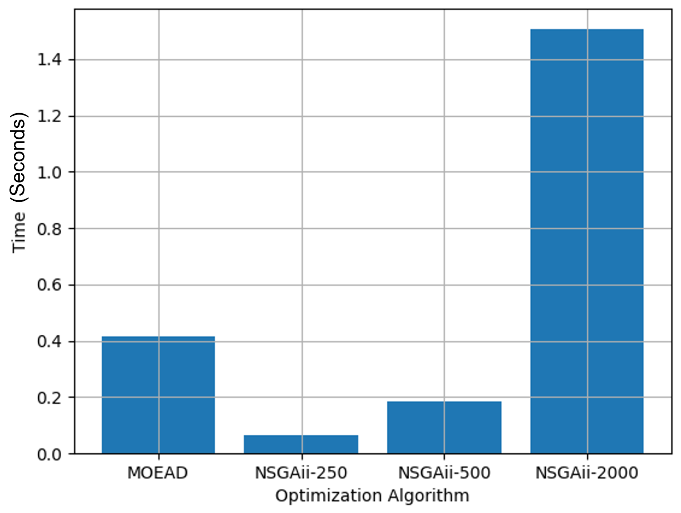
| Simulation Results for Varying Population Size | |||
|---|---|---|---|
| Optimization Algorithm | Time Taken (Seconds) | Area Missed (Metres) | Path Length (Metres) |
| NSGAii (population size—250) | 0.0666 | 0.87 | 16.9 |
| NSGAii (population size—500) | 0.182 | 0.332 | 15.2 |
| NSGAii (population size—2000) | 1.424 | 0.16 | 14.6 |
| MOEA/D (neighboring size—15) | 0.414 | 0.37 | 15.7 |
| Simulation Results for Varying Area Using NSGA2-2000 | ||||
|---|---|---|---|---|
| Test-Bed Size (Metres) | (Metres) | (Metres) | Area Missed (Metres) | Path Length (Metres) |
| 2 × 2 | 1.401 | 0.4951 | 0.19 | 7.089 |
| 3 × 2 | 2.401 | 0.4951 | 0.21 | 11.08 |
| 4 × 2 | 3.401 | 0.4951 | 0.16 | 15.08 |
| Experimental Results for Varying Area Using Solutions from NSGA2-2000 | ||
|---|---|---|
| Test-Bed Size (Metres) | Time Taken (Seconds) | Path Length (Metres) |
| 2 × 2 | 68.37 | 7.452 |
| 3 × 2 | 82.237 | 11.97 |
| 4 × 2 | 117.28 | 15.96 |
Publisher’s Note: MDPI stays neutral with regard to jurisdictional claims in published maps and institutional affiliations. |
© 2021 by the authors. Licensee MDPI, Basel, Switzerland. This article is an open access article distributed under the terms and conditions of the Creative Commons Attribution (CC BY) license (https://creativecommons.org/licenses/by/4.0/).
Share and Cite
Pathmakumar, T.; Sivanantham, V.; Anantha Padmanabha, S.G.; Elara, M.R.; Tun, T.T. Towards an Optimal Footprint Based Area Coverage Strategy for a False-Ceiling Inspection Robot. Sensors 2021, 21, 5168. https://doi.org/10.3390/s21155168
Pathmakumar T, Sivanantham V, Anantha Padmanabha SG, Elara MR, Tun TT. Towards an Optimal Footprint Based Area Coverage Strategy for a False-Ceiling Inspection Robot. Sensors. 2021; 21(15):5168. https://doi.org/10.3390/s21155168
Chicago/Turabian StylePathmakumar, Thejus, Vinu Sivanantham, Saurav Ghante Anantha Padmanabha, Mohan Rajesh Elara, and Thein Than Tun. 2021. "Towards an Optimal Footprint Based Area Coverage Strategy for a False-Ceiling Inspection Robot" Sensors 21, no. 15: 5168. https://doi.org/10.3390/s21155168
APA StylePathmakumar, T., Sivanantham, V., Anantha Padmanabha, S. G., Elara, M. R., & Tun, T. T. (2021). Towards an Optimal Footprint Based Area Coverage Strategy for a False-Ceiling Inspection Robot. Sensors, 21(15), 5168. https://doi.org/10.3390/s21155168