
Low-Cost Eye Tracking Calibration: A Knowledge-Based Study †

 , , , , and
Abstract
:1. Introduction
- A theoretical analysis of the importance of calibration in low-resolution, as well as the necessary features to obtain accurate gaze-estimations in low-resolution.
- Validation of the role of the calibration in a real environment according to the theoretical framework, extending the work proposed in [24] and analyzing the importance of calibration over other methods that enhance gaze-estimation algorithms.
2. Working Framework
2.1. Databases
2.1.1. Theoretical Framework
- Headpose, with position and rotation components.
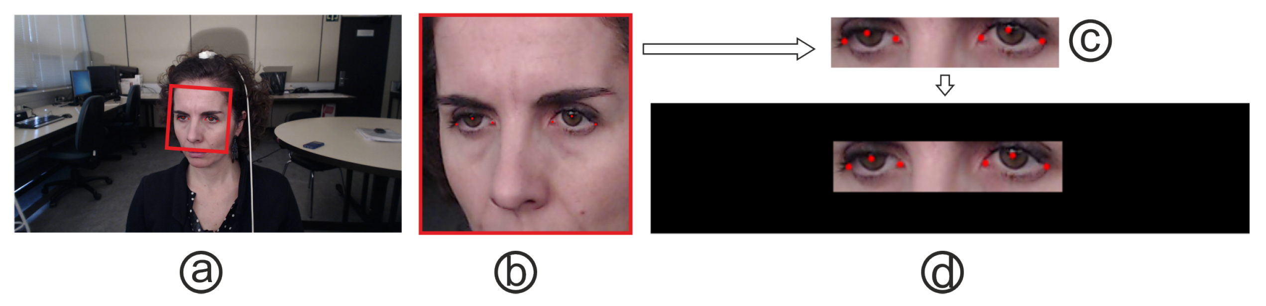
- Tags referred to the location of Points of Interest (PoIs). An example is shown in Figure 2a.
- Landmarks referring to the segmentation of Regions of Interest (RoIs). The RoIs representing the different eye areas are presented in Figure 2b. Both the selected PoIs and RoIs could be extracted from real images, by segmentation tasks (RoIs) or regression (PoIs).
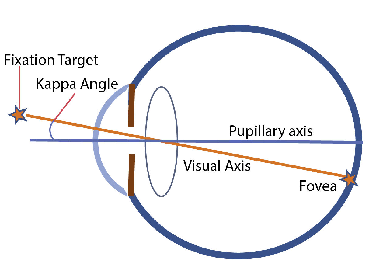
- Kappa angles, with vertical and horizontal components for both eyes. Together with the PCA coefficients (affecting the head shape) and textures (affecting skin and eyes appearance), these are the labels that capture the individuality of each user, i.e., their unique characteristics. Among these 4 components (PCA, kappa angles and skin/eye textures), we understand that it will be mainly the kappa angles and PCA coefficients that will affect the gaze-estimation for each specific user the most. In other words, these would be the features learned during the calibration stage as they represent an individual’s unique characteristics.
- U2Eyes-Base-20. This is a subdatabase with 20 users, each with its own PCA and skin texture, and sharing eye texture in groups of 4. Each of the users has its own kappa angle values, drawn randomly from the distributions characterized by the means and standard deviations from Table 1. Each user presents 125 head positions, and in each head position looks at 32 + 15 grid points. The gaze angle range is ∼°, and the range of the user distances from the grid goes from 35 to 55 cm. This is the range of distances between the eyes and the grid. For more information about the grid points and head pose ranges, see the paper [23].
- U2Eyes-Kappa-20. It is also a subdatabase with 20 users, twins in terms of PCA conditions, skin texture and eyes with the U2Eyes-Base-20 subdatabase, but in this case all users share the same kappa angle values, these being the mean values in Table 1. Head positions and grid points coincide with the ones in the U2Eyes-Base-20 users too.
- U2Eyes-Base-300. Similar to the U2Eyes-Base-20 case, this is a database of 300 users, each of them being a unique user (unique combination of PCA, skin and eye textures). Furthermore, the users present their own kappa angles. In this case, the number of head positions is limited to 27 in the same range of distances, although the gaze angle range is the same as in the previous case, using a grid of 15 points.
- U2Eyes-Kappa-300. As the U2Eyes-Kappa-20 is identical to U2Eyes-Base-20 except for the kappa values of the users, U2Eyes-Kappa-300 is identical to U2Eyes-Base-300 except that all users share the kappa values also used in U2Eyes-Kappa-20.
2.1.2. Real Environment
2.2. Data Processing
2.2.1. Theoretical Framework
- Altering the input to the network to use 4 fewer parameters;
- Applying a uniform random value, in the range −1 to 1, to the values of these features for all users;
2.2.2. Real Environment
2.3. Networks Architecture
2.3.1. Theoretical Framework
- An input layer of 366 inputs, equivalent to the number of features employed;
- Six layers with 512 neurons per layer, ELU activations, using the He uniform variance scaling initializer [33], and kernel regularization l2 with value 0.01 per layer;
- A final layer of 2 neurons, with linear activation, which returns the x and y components of the estimated gaze;
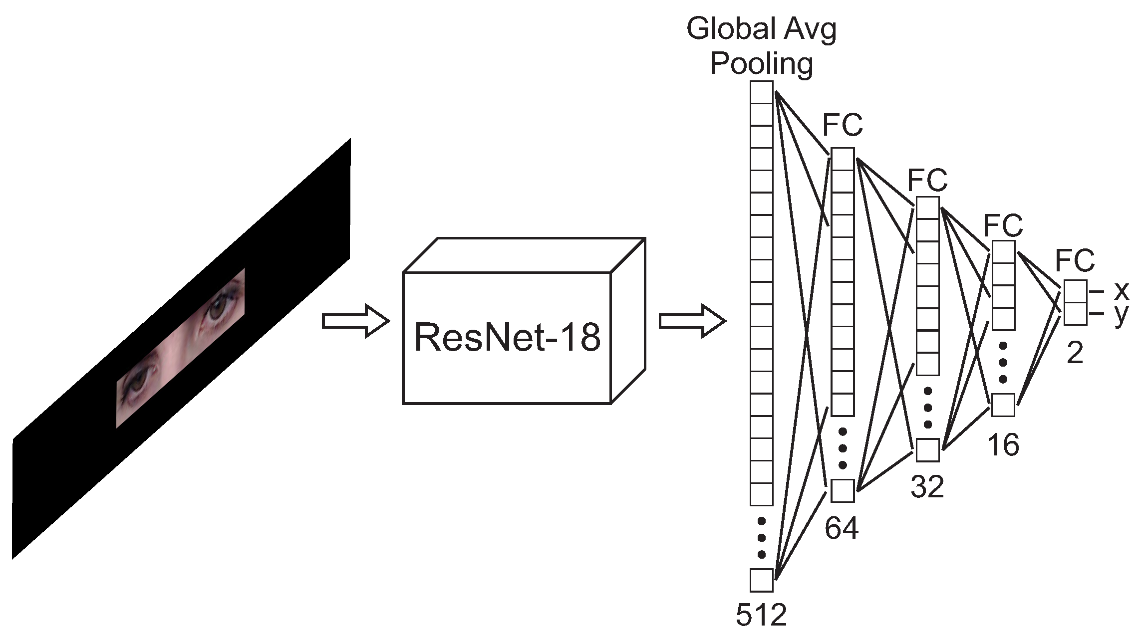
2.3.2. Real Environment
2.4. Implementation Details
2.4.1. Common Characteristics
2.4.2. Theoretical Framework
2.4.3. Real Environment
3. Experiments
3.1. Theoretical Framework
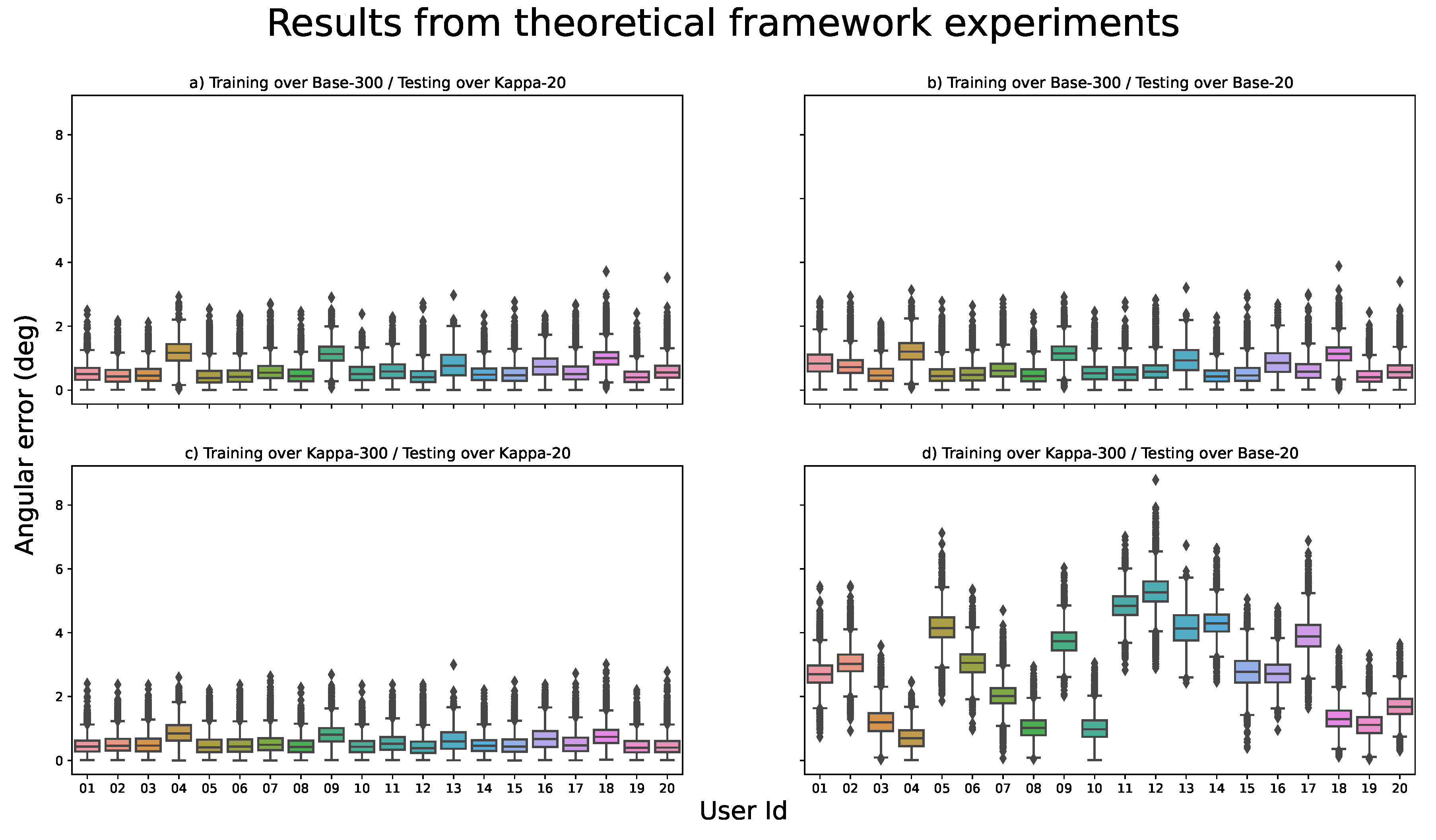
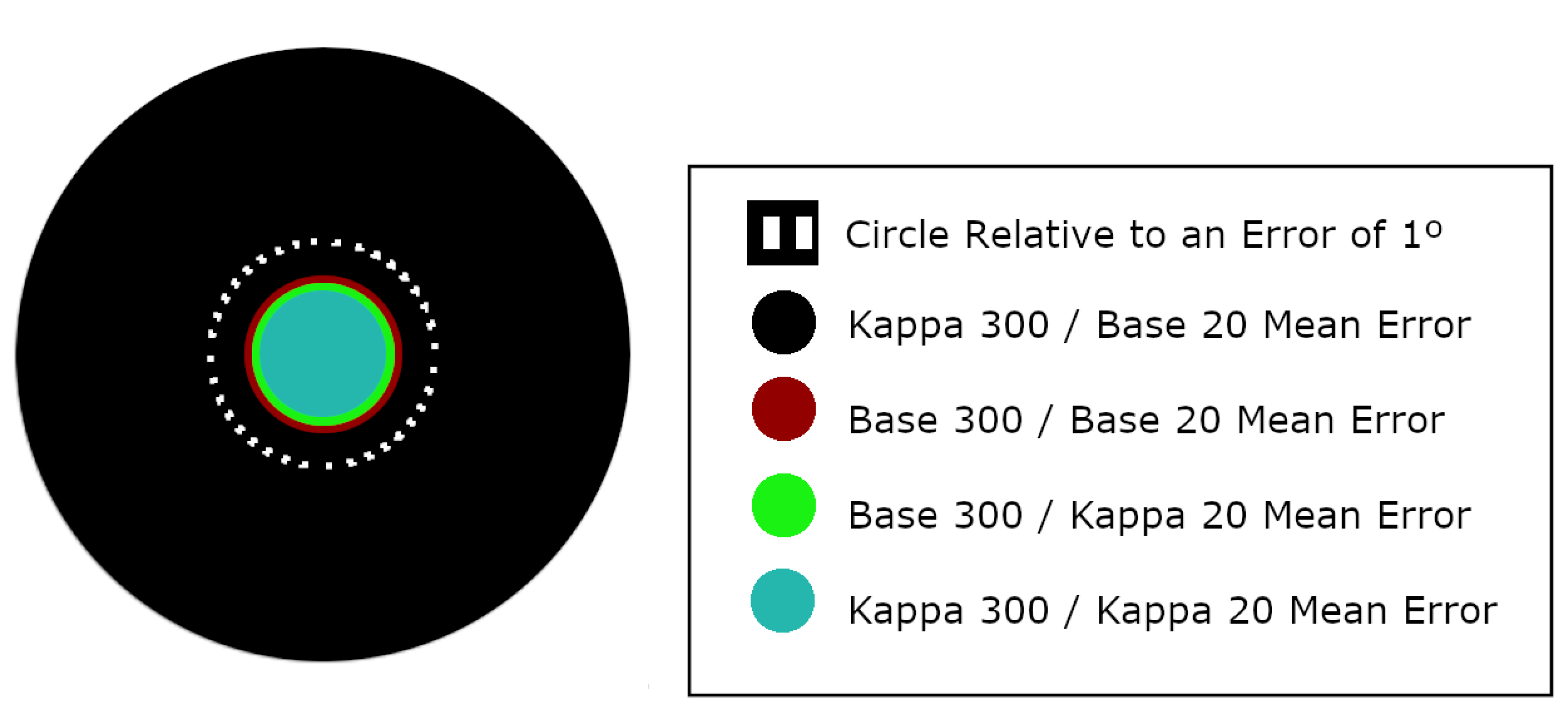
- The network trained on the U2Eyes-Base-300 database should return similar results when tested on either database, since it should learn to interpret the kappa angle values to solve the gaze-estimation.
- The network trained on the U2Eyes-Kappa-300 database should return correct results when tested on the U2Eyes-Kappa-20 database, since both use the same kappa values and the network has learned to solve the gaze-estimation problem for these values, and significantly worse results for the U2Eyes-Base-20 database, since it does not understand the influence that other kappa values have on gaze-estimation.
3.2. Real Environment
3.3. Limitations of the Experiments
- The theoretical framework experiments, as it uses a synthetic framework, have perfectly annotated and controlled features. However, in a real environment, these characteristics present noise due to the labeling process, wherever it is automatic or manual. This added noise will have an effect on the final gaze estimation. To overcome this limitation, it would be necessary to perform an analysis to characterize the noise, so it could be added to the synthetic features.
- In the real environment, we work with a specific dataset where the head motion and boundary conditions (illumination, distance to the grid, static background, etc.) are controlled, as opposed to a “in-the-wild” scenario.
4. Results
4.1. Theoretical Framework
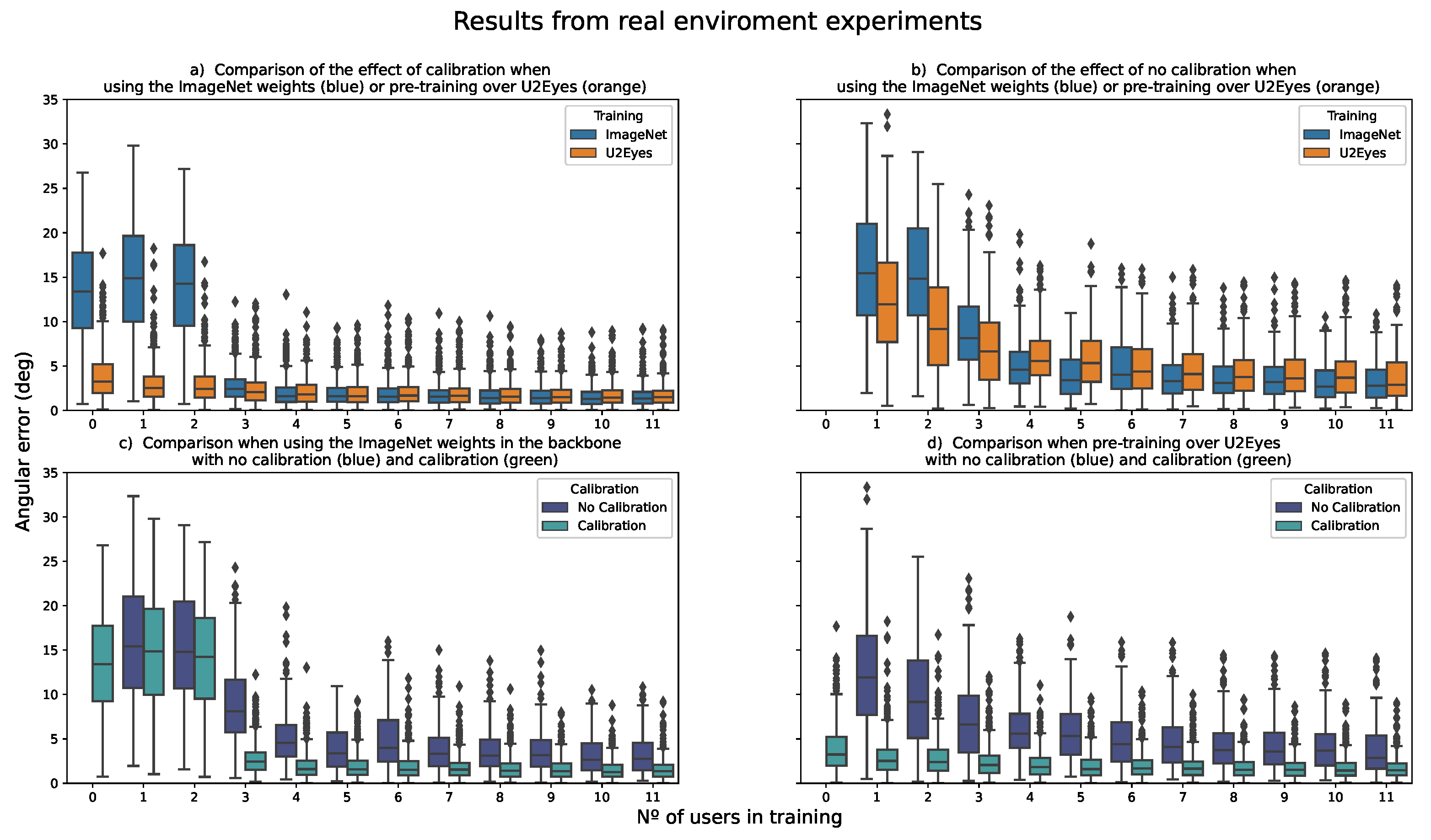
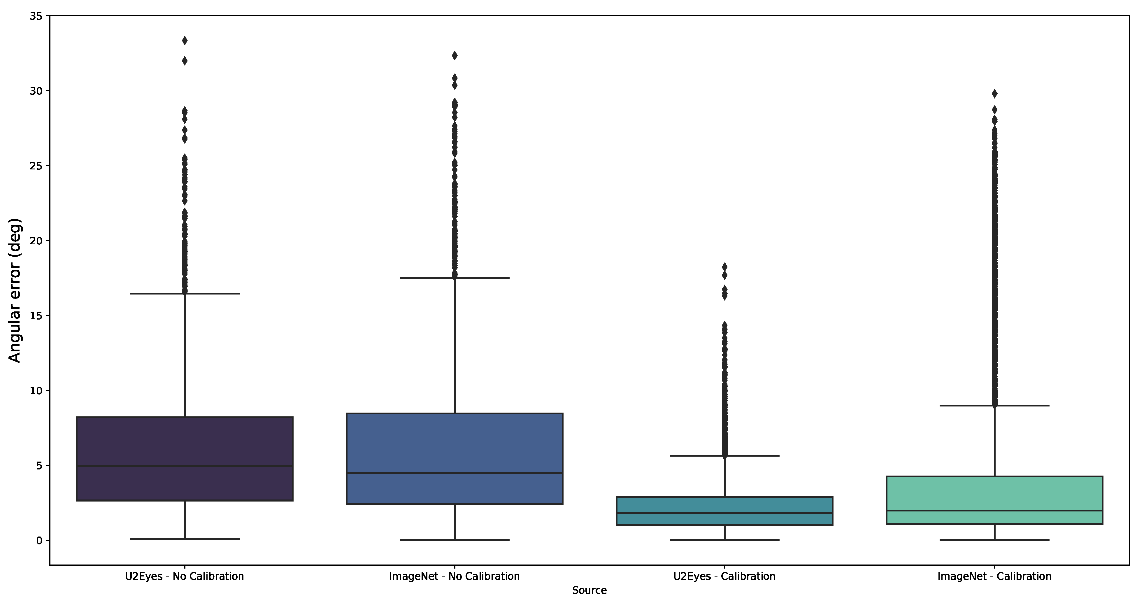
4.2. Real Environment
5. Discussion
5.1. Theoretical Framework
The network trained on the U2Eyes-Base-300 database should return similar results when tested on either database, since it should learn to interpret the kappa angle values to solve the gaze-estimation
The network trained on the U2Eyes-Kappa-300 database should return correct results when tested on the U2Eyes-Kappa-20 database, since both use the same kappa values and the network has learned to solve the gaze-estimation problem for these values, and significantly worse results for the U2Eyes-Base-20 database, since it does not understand the influence that other kappa values have on gaze-estimation
5.2. Real Environment
6. Conclusions
- To try to establish a theoretical framework that shows the influence and impact of calibration in the cases of gaze-estimation for low-resolution, understanding the calibration for fitting the gaze-estimation model to individual and intrinsic conditions of the user. In our case, determined by the kappa parameters of the synthetic environment U2Eyes;
- To check the impact of this calibration on a real database.
Author Contributions
Funding
Institutional Review Board Statement
Informed Consent Statement
Data Availability Statement
Conflicts of Interest
References
- Dosovitskiy, A.; Beyer, L.; Kolesnikov, A.; Weissenborn, D.; Zhai, X.; Unterthiner, T.; Dehghani, M.; Minderer, M.; Heigold, G.; Gelly, S.; et al. An Image is Worth 16 × 16 Words: Transformers for Image Recognition at Scale. In Proceedings of the International Conference on Learning Representations, Vienna, Austria, 3–7 May 2021. [Google Scholar]
- Karras, T.; Laine, S.; Aittala, M.; Hellsten, J.; Lehtinen, J.; Aila, T. Analyzing and Improving the Image Quality of StyleGAN. In Proceedings of the IEEE/CVF Conference on Computer Vision and Pattern Recognition (CVPR), Seattle, WA, USA, 14–19 June 2020. [Google Scholar]
- Bulat, A.; Kossaifi, J.; Tzimiropoulos, G.; Pantic, M. Toward fast and accurate human pose estimation via soft-gated skip connections. In Proceedings of the 2020 15th IEEE International Conference on Automatic Face & Gesture Recognition, Buenos Aires, Argentina, 16–20 November 2020. [Google Scholar]
- Fisher, A.; Rudin, C.; Dominici, F. All Models are Wrong, but Many are Useful: Learning a Variable’s Importance by Studying an Entire Class of Prediction Models Simultaneously. J. Mach. Learn. Res. 2019, 20, 1–81. [Google Scholar]
- Simonyan, K.; Vedaldi, A.; Zisserman, A. Deep Inside Convolutional Networks: Visualising Image Classification Models and Saliency Maps. arXiv 2013, arXiv:1312.6034. [Google Scholar]
- Josifovski, J.; Kerzel, M.; Pregizer, C.; Posniak, L.; Wermter, S. Object Detection and Pose Estimation Based on Convolutional Neural Networks Trained with Synthetic Data. In Proceedings of the 2018 IEEE/RSJ International Conference on Intelligent Robots and Systems (IROS), Madrid, Spain, 1–5 October 2018; pp. 6269–6276. [Google Scholar] [CrossRef]
- Wu, X.; Liang, L.; Shi, Y.; Fomel, S. FaultSeg3D: Using synthetic data sets to train an end-to-end convolutional neural network for 3D seismic fault segmentation. Geophysics 2019, 84, IM35–IM45. [Google Scholar] [CrossRef]
- Le, T.A.; Baydin, A.G.; Zinkov, R.; Wood, F. Using synthetic data to train neural networks is model-based reasoning. In Proceedings of the 2017 International Joint Conference on Neural Networks (IJCNN), Anchorage, AK, USA, 14–19 May 2017; pp. 3514–3521. [Google Scholar] [CrossRef] [Green Version]
- Garde, G.; Larumbe-Bergera, A.; Bossavit, B.; Cabeza, R.; Porta, S.; Villanueva, A. Gaze Estimation Problem Tackled through Synthetic Images. In Proceedings of the ACM Symposium on Eye Tracking Research and Applications, Association for Computing Machinery, Stuttgart, Germany, 2–5 June 2020. [Google Scholar] [CrossRef]
- He, J.; Pham, K.; Valliappan, N.; Xu, P.; Roberts, C.; Lagun, D.; Navalpakkam, V. On-Device Few-Shot Personalization for Real-Time Gaze Estimation. In Proceedings of the 2019 IEEE International Conference on Computer Vision (ICCV) Workshops, Seoul, Korea, 27 October–2 November 2019. [Google Scholar]
- Guo, T.; Liu, Y.; Zhang, H.; Liu, X.; Kwak, Y.; In Yoo, B.; Han, J.J.; Choi, C. A Generalized and Robust Method Towards Practical Gaze Estimation on Smart Phone. In Proceedings of the 2019 International Conference on Computer Vision (ICCV) Workshops, Seoul, Korea, 27 October–2 November 2019. [Google Scholar]
- Yu, Y.; Odobez, J.M. Unsupervised Representation Learning for Gaze Estimation. In Proceedings of the IEEE/CVF Conference on Computer Vision and Pattern Recognition (CVPR), Seattle, WA, USA, 14–19 June 2020. [Google Scholar]
- Villanueva, A.; Cabeza, R.; Porta, S. Eye Tracking System Model with Easy Calibration. In Proceedings of the 2004 Symposium on Eye Tracking Research & Applications, Association for Computing Machinery, San Antonio, TX, USA, 22–24 March 2004; p. 55. [Google Scholar] [CrossRef]
- Pfeuffer, K.; Vidal, M.; Turner, J.; Bulling, A.; Gellersen, H. Pursuit Calibration: Making Gaze Calibration Less Tedious and More Flexible. In Proceedings of the 26th Annual ACM Symposium on User Interface Software and Technology, Association for Computing Machinery, St Andrews, UK, 8–11 October 2013; pp. 261–270. [Google Scholar] [CrossRef]
- Drewes, H.; Pfeuffer, K.; Alt, F. Time- and Space-Efficient Eye Tracker Calibration. In Proceedings of the 11th ACM Symposium on Eye Tracking Research & Applications, Association for Computing Machinery, Denver, CO, USA, 25–28 June 2019. [Google Scholar] [CrossRef] [Green Version]
- Gomez, A.R.; Gellersen, H. Smooth-i: Smart Re-Calibration Using Smooth Pursuit Eye Movements. In Proceedings of the 2018 ACM Symposium on Eye Tracking Research & Applications, Association for Computing Machinery, Warsaw, Poland, 14–17 June 2018. [Google Scholar] [CrossRef] [Green Version]
- Morimoto, C.H.; Mimica, M.R. Eye gaze tracking techniques for interactive applications. Comput. Vis. Image Underst. 2005, 98, 4–24, Special Issue on Eye Detection and Tracking. [Google Scholar] [CrossRef]
- Park, S.; Mello, S.D.; Molchanov, P.; Iqbal, U.; Hilliges, O.; Kautz, J. Few-Shot Adaptive Gaze Estimation. In Proceedings of the IEEE/CVF International Conference on Computer Vision (ICCV), Seoul, Korea, 27 October–2 November 2019. [Google Scholar]
- Linden, E.; Sjostrand, J.; Proutiere, A. Learning to Personalize in Appearance-Based Gaze Tracking. In Proceedings of the the IEEE International Conference on Computer Vision (ICCV) Workshops, Seoul, Korea, 27 October–2 November 2019. [Google Scholar]
- Chen, Z.; Shi, B. Offset Calibration for Appearance-Based Gaze Estimation via Gaze Decomposition. In Proceedings of the IEEE/CVF Winter Conference on Applications of Computer Vision (WACV), Snowmass Village, CO, USA, 1–5 March 2020. [Google Scholar]
- Gudi, A.; Li, X.; van Gemert, J. Efficiency in Real-Time Webcam Gaze Tracking. In Proceedings of the European Conference on Computer Vision, ECCV, Glasgow, UK, 23–28 August 2020. [Google Scholar]
- Liu, G.; Yu, Y.; Funes Mora, K.A.; Odobez, J.M. A Differential Approach for Gaze Estimation. IEEE Trans. Pattern Anal. Mach. Intell. 2019, 43, 1092–1099. [Google Scholar] [CrossRef] [PubMed] [Green Version]
- Porta, S.; Bossavit, B.; Cabeza, R.; Larumbe-Bergera, A.; Garde, G.; Villanueva, A. U2Eyes: A Binocular Dataset for Eye Tracking and Gaze Estimation. In Proceedings of the 2019 IEEE International Conference on Computer Vision (ICCV), Seoul, Korea, 27 October–3 November 2019. [Google Scholar]
- Garde, G.; Larumbe-Bergera, A.; Porta, S.; Cabeza, R.; Villanueva, A. Synthetic Gaze Data Augmentation for Improved User Calibration. In Proceedings of the 2021 International Conference on Pattern Recognition 2020 (ICPR), Milano, Italy, 10–15 January 2021; pp. 377–389. [Google Scholar] [CrossRef]
- Wood, E.; Baltrušaitis, T.; Morency, L.P.; Robinson, P.; Bulling, A. Learning an appearance-based gaze estimator from one million synthesised images. In Proceedings of the Ninth Biennial ACM Symposium on Eye Tracking Research & Applications, Charleston, SC, USA, 14–18 March 2016; pp. 131–138. [Google Scholar]
- Abass, A.; Vinciguerra, R.; Lopes, B.T.; Bao, F.; Vinciguerra, P.; Jr, R.A.; Elsheikh, A. Positions of Ocular Geometrical and Visual Axes in Brazilian, Chinese and Italian Populations. Curr. Eye Res. 2018, 43, 1404–1414. [Google Scholar] [CrossRef] [PubMed] [Green Version]
- Velasco-Barona, C.; Corredor-Ortega, C.; Mendez-Leon, A.; Casillas-Chavarín, N.L.; Valdepeña-López Velarde, D.; Cervantes-Coste, G.; Malacara-Hernández, D.; Gonzalez-Salinas, R. Influence of Angle κ and Higher-Order Aberrations on Visual Quality Employing Two Diffractive Trifocal IOLs. J. Ophthalmol. 2019, 2019, 7018937. [Google Scholar] [CrossRef] [PubMed]
- Cameron, J.R.; Megaw, R.D.; Tatham, A.J.; McGrory, S.; MacGillivray, T.J.; Doubal, F.N.; Wardlaw, J.M.; Trucco, E.; Chandran, S.; Dhillon, B. Lateral thinking—Interocular symmetry and asymmetry in neurovascular patterning, in health and disease. Prog. Retin. Eye Res. 2017, 59, 131–157. [Google Scholar] [CrossRef] [PubMed] [Green Version]
- Krafka, K.; Khosla, A.; Kellnhofer, P.; Kannan, H.; Bhandarkar, S.; Matusik, W.; Torralba, A. Eye tracking for everyone. In Proceedings of the IEEE Conference on Computer Vision and Pattern Recognition, Vegas, NV, USA, 27–30 June 2016; pp. 2176–2184. [Google Scholar]
- Zhang, X.; Sugano, Y.; Fritz, M.; Bulling, A. Appearance-based gaze estimation in the wild. In Proceedings of the 2015 IEEE Conference on Computer Vision and Pattern Recognition (CVPR), Boston, MA, USA, 7–12 June 2015; pp. 4511–4520. [Google Scholar] [CrossRef] [Green Version]
- Zhang, X.; Park, S.; Beeler, T.; Bradley, D.; Tang, S.; Hilliges, O. ETH-XGaze: A Large Scale Dataset for Gaze Estimation under Extreme Head Pose and Gaze Variation. In Proceedings of the European Conference on Computer Vision 2020, ECCV, Glasgow, UK, 23–28 August 2020. [Google Scholar]
- Martinikorena, I.; Cabeza, R.; Villanueva, A.; Porta, S. Introducing I2Head database. In Proceedings of the 7th International Workshop on Pervasive Eye Tracking and Mobile Eye-based Interaction, PETMEI@ETRA 2018, Warsaw, Poland, 15–16 June 2018. [Google Scholar]
- He, K.; Zhang, X.; Ren, S.; Sun, J. Delving Deep into Rectifiers: Surpassing Human-Level Performance on ImageNet Classification. In Proceedings of the IEEE International Conference on Computer Vision (ICCV), Santiago, Chile, 13–16 December 2015. [Google Scholar]
- Deng, J.; Dong, W.; Socher, R.; Li, L.J.; Li, K.; Fei-Fei, L. ImageNet: A Large-Scale Hierarchical Image Database. In Proceedings of the 2009 IEEE Conference on Computer Vision and Pattern Recognition, CVPR09, Miami, FL, USA, 20–25 June 2009. [Google Scholar]
- Smith, L.N. Cyclical Learning Rates for Training Neural Networks. In Proceedings of the 2017 IEEE Winter Conference on Applications of Computer Vision (WACV), Santa Rosa, CA, USA, 27–29 March 2017. [Google Scholar]
- Zhang, X.; Sugano, Y.; Fritz, M.; Bulling, A. It’s Written All Over Your Face: Full-Face Appearance-Based Gaze Estimation. In Proceedings of the IEEE Conference on Computer Vision and Pattern Recognition Workshops, Honolulu, HI, USA, 21–26 July 2017; pp. 2299–2308. [Google Scholar]
- Zhu, W.; Deng, H. Monocular Free-Head 3D Gaze Tracking with Deep Learning and Geometry Constraints. In Proceedings of the IEEE International Conference on Computer Vision (ICCV), Venice, Italy, 22–29 October 2017. [Google Scholar]


| Kappa Angle | Horizontal Right | Vertical Right | Horizontal Left | Vertical Left |
|---|---|---|---|---|
| Mean | 5.4237 | 2.512 | 2.1375 | 4.4458 |
| Std | 2.4978 | 2.6782 | 1.9672 | 2.7185 |
| Model | Train # Users/Images | Calibration # Users/Images | Total Train # Images | Test # Users/Images |
|---|---|---|---|---|
| ImageNet | K/K × 130 | 1/34 | K × 130 + 34 | 1/130 |
| U2Eyes | K/K × 130 | 1/34 | K × 130 + 34 | 1/130 |
| Model | Train # Users/Images | Total Train # Images | Test # Users/Images |
|---|---|---|---|
| ImageNet | K/K × 130 | K × 130 | 1/130 |
| U2Eyes | K/K × 130 | K × 130 | 1/130 |
| Training Database | U2Eyes-Base-300 | U2Eyes-Kappa-300 | ||
|---|---|---|---|---|
| Testing Database | U2Eyes-Kappa-20 | U2Eyes-Base-20 | U2Eyes-Kappa-20 | U2Eyes-Base-20 |
| N° Samples | 117,500 | 117,500 | 117,500 | 117,500 |
| Mean | 0.639 | 0.709 | 0.566 | 2.749 |
| Std | 0.393 | 0.419 | 0.342 | 1.462 |
| Min | 0.001 | 0.001 | 0.001 | 0.008 |
| 25% | 0.342 | 0.390 | 0.311 | 1.399 |
| 50% | 0.556 | 0.628 | 0.501 | 2.753 |
| 75% | 0.866 | 0.963 | 0.753 | 3.927 |
| Max | 3.716 | 3.885 | 3.014 | 8.788 |
| Mean | Median | |||||||
|---|---|---|---|---|---|---|---|---|
| Model | ImageNet | ImageNet | U2Eyes | U2Eyes | ImageNet | ImageNet | U2Eyes | U2Eyes |
| Calibration | Yes | No | Yes | No | Yes | No | Yes | No |
| Users in training | ||||||||
| 0 | 13,615 | None | 3891 | None | 13,401 | None | 3243 | None |
| 1 | 14,812 | 16,133 | 2967 | 12,656 | 14,880 | 15,446 | 2522 | 11,935 |
| 2 | 14,069 | 15,456 | 2861 | 9982 | 14,255 | 14,807 | 2404 | 9169 |
| 3 | 2710 | 9160 | 2376 | 7387 | 2426 | 8126 | 2061 | 6626 |
| 4 | 1918 | 5278 | 2106 | 6158 | 1598 | 4561 | 1814 | 5572 |
| 5 | 1934 | 3998 | 191 | 5893 | 1586 | 3389 | 1599 | 5326 |
| 6 | 1883 | 4940 | 1963 | 4945 | 1541 | 4001 | 1672 | 4394 |
| 7 | 1770 | 3853 | 1887 | 4726 | 1544 | 3310 | 1648 | 4090 |
| 8 | 1660 | 3773 | 1784 | 4367 | 1397 | 3098 | 1535 | 3736 |
| 9 | 1621 | 3797 | 1748 | 4120 | 1384 | 3182 | 1510 | 3582 |
| 10 | 1541 | 3261 | 1723 | 4260 | 1267 | 2656 | 1446 | 3681 |
| 11 | 1559 | 3302 | 1714 | 3791 | 1344 | 2770 | 1486 | 2866 |
Publisher’s Note: MDPI stays neutral with regard to jurisdictional claims in published maps and institutional affiliations. |
© 2021 by the authors. Licensee MDPI, Basel, Switzerland. This article is an open access article distributed under the terms and conditions of the Creative Commons Attribution (CC BY) license (https://creativecommons.org/licenses/by/4.0/).
Share and Cite
Garde, G.; Larumbe-Bergera, A.; Bossavit, B.; Porta, S.; Cabeza, R.; Villanueva, A. Low-Cost Eye Tracking Calibration: A Knowledge-Based Study. Sensors 2021, 21, 5109. https://doi.org/10.3390/s21155109
Garde G, Larumbe-Bergera A, Bossavit B, Porta S, Cabeza R, Villanueva A. Low-Cost Eye Tracking Calibration: A Knowledge-Based Study. Sensors. 2021; 21(15):5109. https://doi.org/10.3390/s21155109
Chicago/Turabian StyleGarde, Gonzalo, Andoni Larumbe-Bergera, Benoît Bossavit, Sonia Porta, Rafael Cabeza, and Arantxa Villanueva. 2021. "Low-Cost Eye Tracking Calibration: A Knowledge-Based Study" Sensors 21, no. 15: 5109. https://doi.org/10.3390/s21155109
APA StyleGarde, G., Larumbe-Bergera, A., Bossavit, B., Porta, S., Cabeza, R., & Villanueva, A. (2021). Low-Cost Eye Tracking Calibration: A Knowledge-Based Study. Sensors, 21(15), 5109. https://doi.org/10.3390/s21155109