
Deep and Wide Transfer Learning with Kernel Matching for Pooling Data from Electroencephalography and Psychological Questionnaires

 ,
,
Abstract
:1. Introduction
2. Materials and Methods
2.1. 2D Feature Representation of EEG Data
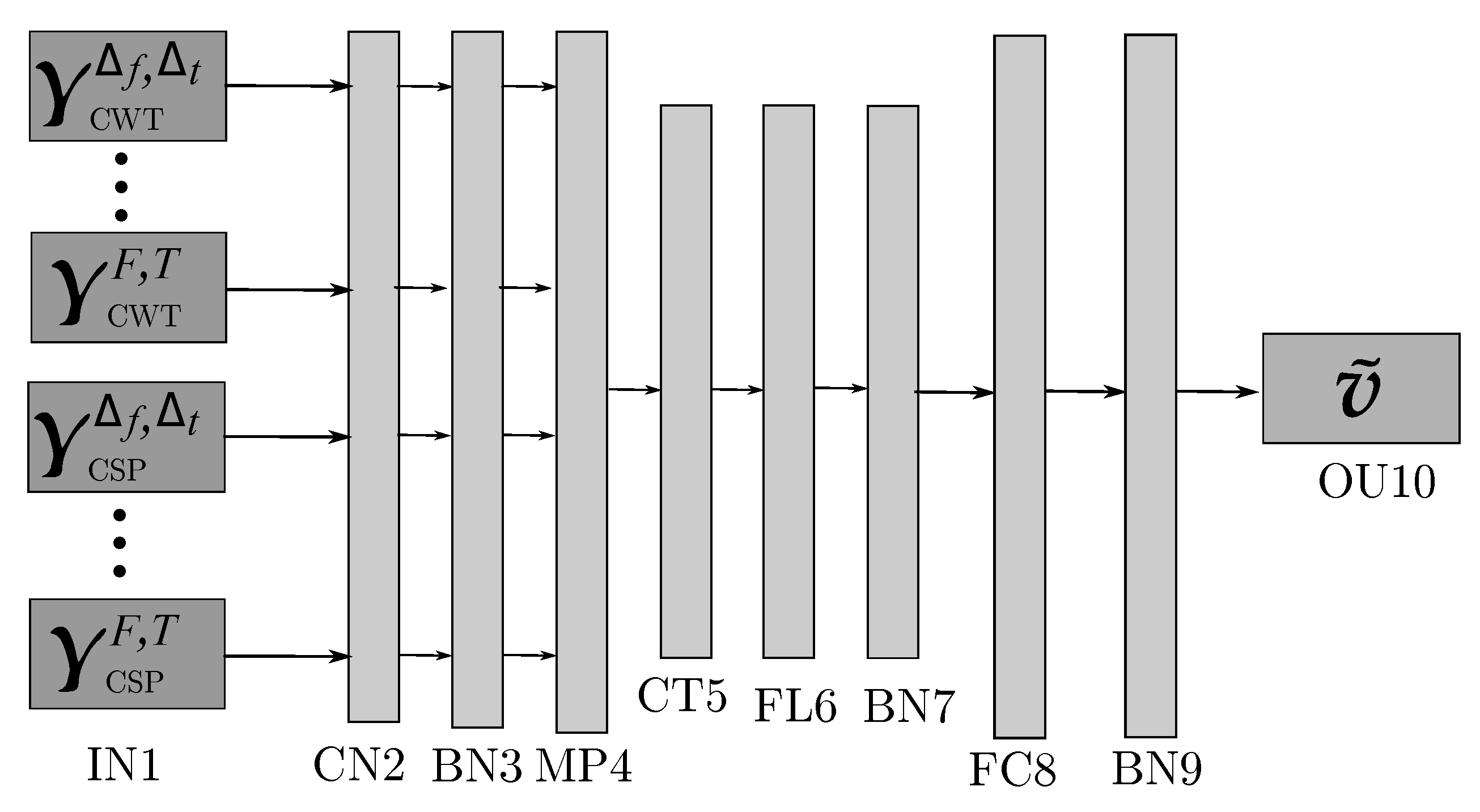
2.2. Multi-Layer Perceptron Classifier Using 2D Feature Representation
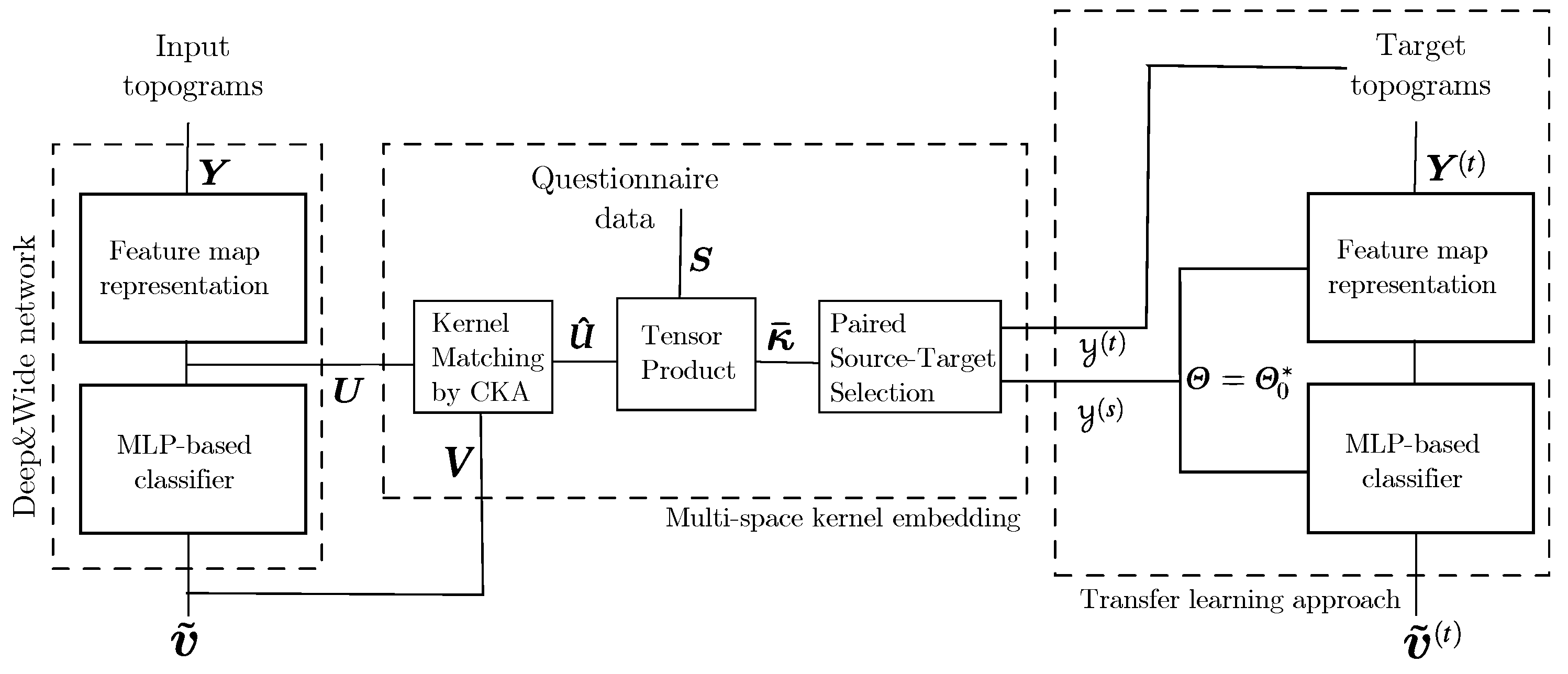
2.3. Transfer Learning with Added Questionnaire Data
3. Experimental Set-Up
3.1. Database Description and Preprocessing
3.2. MLP Classifier Performance Fed by 2D Features
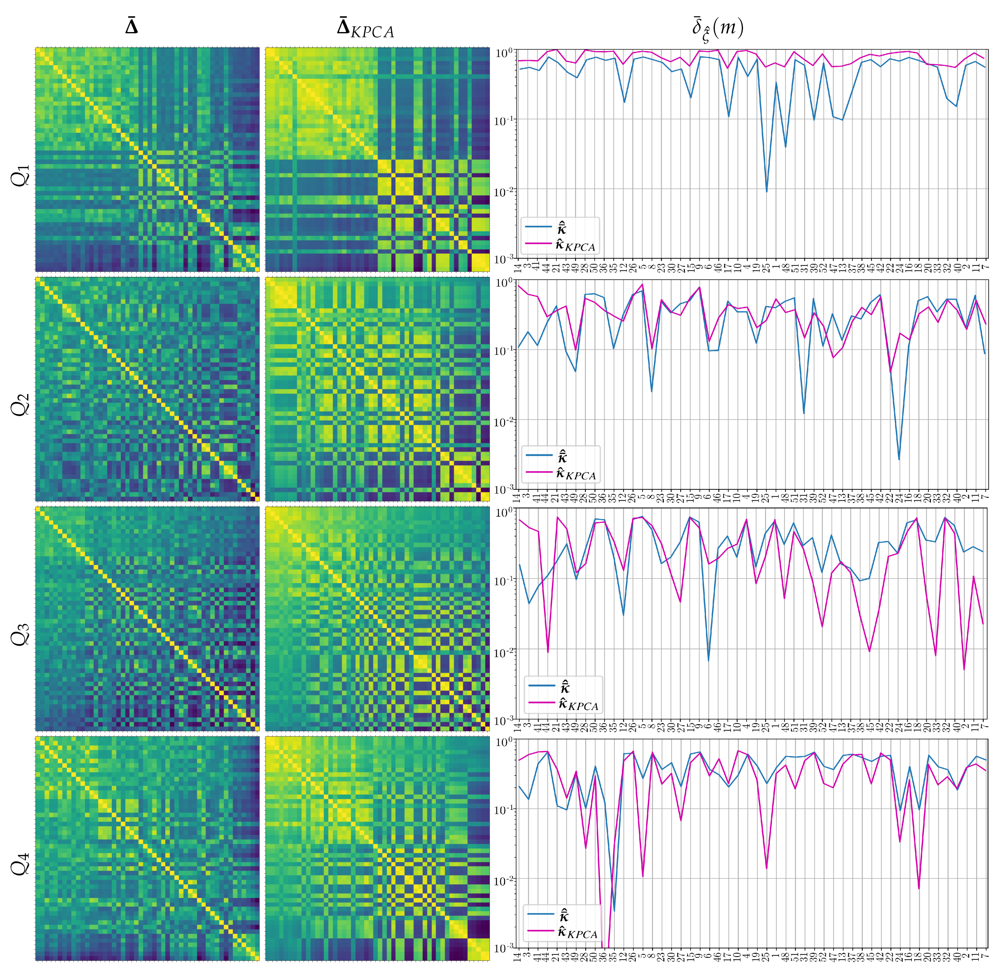
3.3. Performed Stepwise Multi-Space Kernel Matching
| Algorithm 1 Validation procedure of the proposed approach for transfer learning with stepwise, multi-space kernel matching. Dimensionality reduction is an optional procedure performed for comparison purposes. |
Input data: EEG measurement , predicted label probabilities , questionary data
|
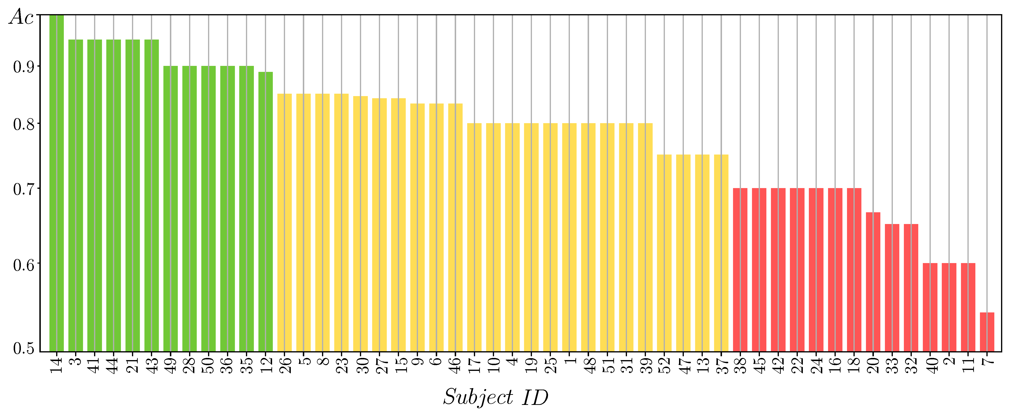
3.4. Estimation of Pre-Trained Weights for Cross-Subject Transfer Learning
- (a)
- Single source-single-target, when we select the subject of Group I, achieving the highest value of the domain distance measurement in Equation (9) computed as follows:Once the source-target pairs are selected, the pre-trained weights are computed from each designed source subject to initialize the Deep and Wide neural network, rather than introducing a zero-valued starting iterate, and thus enabling a better convergence of the training algorithm. Note that the fulfilling condition in Equation (9) depends on , meaning distinct selected sources for each questionnaire data.
- (b)
- Multiple sources-single-target when the selected subjects of Group I achieve the four highest domain distance values. In this case, the Deep and Wide initialization procedure applies the pre-trained weights estimated from the concatenation of the source topograms.
4. Discussion and Concluding Remarks
Author Contributions
Funding
Informed Consent Statement
Data Availability Statement
Conflicts of Interest
References
- Ladda, A.; Lebon, F.; Lotze, M. Using motor imagery practice for improving motor performance—A review. Brain Cogn. 2021, 150, 105705. [Google Scholar] [CrossRef] [PubMed]
- James, C.; Zuber, S.; Dupuis Lozeron, E.; Abdili, L.; Gervaise, D.; Kliegel, M. How Musicality, Cognition and Sensorimotor Skills Relate in Musically Untrained Children. Swiss J. Psychol. 2020, 79, 101–112. [Google Scholar] [CrossRef]
- Basso, J.; Satyal, M.; Rugh, R. Dance on the Brain: Enhancing Intra- and Inter-Brain Synchrony. Front. Hum. Neurosci. 2021, 14, 586. [Google Scholar] [CrossRef]
- Suggate, S.; Martzog, P. Screen-time influences children’s mental imagery performance. Dev. Sci. 2020, 23, e12978. [Google Scholar] [CrossRef] [PubMed]
- Bahmani, M.; Babak, M.; Land, W.; Howard, J.; Diekfuss, J.; Abdollahipour, R. Children’s motor imagery modality dominance modulates the role of attentional focus in motor skill learning. Hum. Movem. Sci. 2020, 75, 102742. [Google Scholar] [CrossRef]
- Souto, D.; Cruz, T.; Fontes, P.; Batista, R.; Haase, V. Motor Imagery Development in Children: Changes in Speed and Accuracy With Increasing Age. Front. Pediatr. 2020, 8, 100. [Google Scholar] [CrossRef] [Green Version]
- Simpson, T.; Ellison, P.; Carnegie, E.; Marchant, D. A systematic review of motivational and attentional variables on children’s fundamental movement skill development: The OPTIMAL theory. Int. Rev. Sport Exer. Psychol. 2020, 1–47. [Google Scholar] [CrossRef]
- Singh, A.; Hussain, A.; Lal, S.; Guesgen, H. A Comprehensive Review on Critical Issues and Possible Solutions of Motor Imagery Based Electroencephalography brain–computer Interface. Sensors 2021, 21, 2173. [Google Scholar] [CrossRef] [PubMed]
- Al-Saegh, A.; Dawwd, S.; Abdul-Jabbar, J. Deep learning for motor imagery EEG-based classification: A review. Biomed. Signal Process. Control 2021, 63, 102172. [Google Scholar] [CrossRef]
- Thompson, M. Critiquing the Concept of BCI Illiteracy. Sci. Eng. Ethics 2019, 25, 1217–1233. [Google Scholar] [CrossRef] [PubMed]
- McAvinue, L.; Robertson, I. Measuring motor imagery ability: A review. Eur. J. Cogn. Psychol. 2008, 20, 232–251. [Google Scholar] [CrossRef]
- Yoon, J.; Lee, M. Effective Correlates of Motor Imagery Performance based on Default Mode Network in Resting-State. In Proceedings of the 2020 8th International Winter Conference on brain–computer Interface (BCI), Gangwon, Korea, 26–28 February 2020; pp. 1–5. [Google Scholar]
- Rimbert, S.; Gayraud, N.; Bougrain, L.; Clerc, M.; Fleck, S. Can a Subjective Questionnaire Be Used as brain–computer Interface Performance Predictor? Front. Hum. Neurosci. 2019, 12, 529. [Google Scholar] [CrossRef] [PubMed] [Green Version]
- Vasilyev, A.; Liburkina, S.; Yakovlev, L.; Perepelkina, O.; Kaplan, A. Assessing motor imagery in brain–computer interface training: Psychological and neurophysiological correlates. Neuropsychologia 2017, 97, 56–65. [Google Scholar] [CrossRef]
- Seo, S.; Lee, M.; Williamson, J.; Lee, S. Changes in Fatigue and EEG Amplitude during a Longtime Use of brain–computer Interface. In Proceedings of the 2019 7th International Winter Conference on brain–computer Interface (BCI), Gangwon, Korea, 18–20 February 2019; pp. 1–3. [Google Scholar]
- Lioi, G.; Cury, C.; Perronnet, L.; Mano, M.; Bannier, E.; Lécuyer, A.; Barillot, C. Simultaneous MRI-EEG during a motor imagery neurofeedback task: An open access brain imaging dataset for multi-modal data integration. bioRxiv 2019, 2019, 862375. [Google Scholar]
- Collet, C.; Hajj, M.E.; Chaker, R.; Bui-xuan, B.; Lehot, J.; Hoyek, N. Effect of motor imagery and actual practice on learning professional medical skills. BMC Med. Educ. 2021, 21, 59. [Google Scholar] [CrossRef]
- Dähne, S.; Bießmann, F.; Samek, W.; Haufe, S.; Goltz, D.; Gundlach, C.; Villringer, A.; Fazli, S.; Müller, K. Multivariate Machine Learning Methods for Fusing Multimodal Functional Neuroimaging Data. Proc. IEEE 2015, 103, 1507–1530. [Google Scholar] [CrossRef]
- Dai, C.; Wang, Z.; Wei, L.; Chen, G.; Chen, B.; Zuo, F.; Li, Y. Combining early post-resuscitation EEG and HRV features improves the prognostic performance in cardiac arrest model of rats. Am. J. Emerg. Med. 2018, 36, 2242–2248. [Google Scholar] [CrossRef] [PubMed]
- Xu, J.; Zheng, H.; Wang, J.; Li, D.; Fang, X. Recognition of EEG Signal Motor Imagery Intention Based on Deep Multi-View Feature Learning. Sensors 2020, 20, 3496. [Google Scholar] [CrossRef]
- Zhuang, M.; Wu, Q.; Wan, F.; Hu, Y. State-of-the-art non-invasive brain–computer interface for neural rehabilitation: A review. J. Neurorestoratol. 2020, 8, 4. [Google Scholar] [CrossRef] [Green Version]
- Wu, D.; Jiang, X.; Peng, R.; Kong, W.; Huang, J.; Zeng, Z. Transfer Learning for Motor Imagery Based brain–computer Interfaces: A Complete Pipeline. arXiv 2021, arXiv:eess.SP/2007.03746. [Google Scholar]
- Zheng, M.; Yang, B.; Xie, Y. EEG classification across sessions and across subjects through transfer learning in motor imagery-based brain-machine interface system. Med. Biol. Eng. Comput. 2020, 58, 1515–1528. [Google Scholar] [CrossRef]
- Wan, Z.; Yang, R.; Huang, M.; Zeng, N.; Liu, X. A review on transfer learning in EEG signal analysis. Neurocomputing 2021, 421, 1–14. [Google Scholar] [CrossRef]
- Zhang, R.; Zong, Q.; Dou, L.; Zhao, X.; Tang, Y.; Li, Z. Hybrid deep neural network using transfer learning for EEG motor imagery decoding. Biomed. Sig. Process. Control 2021, 63, 102144. [Google Scholar] [CrossRef]
- Kant, P.; Laskar, S.; Hazarika, J.; Mahamune, R. CWT Based Transfer Learning for Motor Imagery Classification for Brain computer Interfaces. J. Neurosci. Methods 2020, 345, 108886. [Google Scholar] [CrossRef] [PubMed]
- Zhang, K.; Robinson, N.; Lee, S.; Guan, C. Adaptive transfer learning for EEG motor imagery classification with deep Convolutional Neural Network. Neural Netw. 2021, 136, 1–10. [Google Scholar] [CrossRef] [PubMed]
- Wei, X.; Ortega, P.; Faisal, A. Inter-subject Deep Transfer Learning for Motor Imagery EEG Decoding. arXiv 2021, arXiv:cs.LG/2103.05351. [Google Scholar]
- Zheng, M.; Yang, B.; Gao, S.; Meng, X. Spatio-time-frequency joint sparse optimization with transfer learning in motor imagery-based brain-computer interface system. Biomed. Signal Process. Control 2021, 68, 102702. [Google Scholar] [CrossRef]
- Zhang, K.; Xu, G.; Chen, L.; Tian, P.; Han, C.; Zhang, S.; Duan, N. Instance transfer subject-dependent strategy for motor imagery signal classification using deep convolutional neural networks. Comput. Math. Methods Med. 2020, 2020. [Google Scholar] [CrossRef] [PubMed]
- Luo, W.; Zhang, J.; Feng, P.; Yu, D.; Wu, Z. A concise peephole model based transfer learning method for small sample temporal feature-based data-driven quality analysis. Knowl. Based Syst. 2020, 195, 105665. [Google Scholar] [CrossRef]
- Zhang, K.; Xu, G.; Zheng, X.; Li, H.; Zhang, S.; Yu, Y.; Liang, R. Application of Transfer Learning in EEG Decoding Based on brain–computer Interfaces: A Review. Sensors 2020, 20, 6321. [Google Scholar] [CrossRef]
- Tan, C.; Sun, F.; Kong, T.; Zhang, W.; Yang, C.; Liu, C. A Survey on Deep Transfer Learning. In Artificial Neural Networks and Machine Learning—ICANN 2018; Kůrková, V., Manolopoulos, Y., Hammer, B., Iliadis, L., Maglogiannis, I., Eds.; Springer International Publishing: Cham, Switzerland, 2018; pp. 270–279. [Google Scholar]
- Zhao, D.; Tang, F.; Si, B.; Feng, X. Learning joint space–time–frequency features for EEG decoding on small labeled data. Neural Netw. 2019, 114, 67–77. [Google Scholar] [CrossRef] [PubMed]
- Parvan, M.; Ghiasi, A.R.; Rezaii, T.; Farzamnia, A. Transfer Learning based Motor Imagery Classification using Convolutional Neural Networks. In Proceedings of the 2019 27th Iranian Conference on Electrical Engineering (ICEE), Yazd, Iran, 30 April–2 May 2019; pp. 1825–1828. [Google Scholar]
- Collazos-Huertas, D.; Álvarez-Meza, A.; Acosta-Medina, C.; Castaño-Duque, G.; Castellanos-Dominguez, G. CNN-based framework using spatial dropping for enhanced interpretation of neural activity in motor imagery classification. Brain Inf. 2020, 7, 8. [Google Scholar] [CrossRef] [PubMed]
- Collazos-Huertas, D.; Álvarez-Meza, A.; Castellanos-Dominguez, G. Spatial interpretability of time-frequency relevance optimized in motor imagery discrimination using Deep and Wide networks. Biomed. Sig. Process. Control 2021, 68, 102626. [Google Scholar] [CrossRef]
- Mammone, N.; Ieracitano, C.; Morabito, F. A deep CNN approach to decode motor preparation of upper limbs from time–frequency maps of EEG signals at source level. Neural Netw. 2020, 124, 357–372. [Google Scholar] [CrossRef]
- Song, L.; Fukumizu, K.; Gretton, A. kernel-embeddings of Conditional Distributions: A Unified Kernel Framework for Nonparametric Inference in Graphical Models. IEEE Signal Process. Mag. 2013, 30, 98–111. [Google Scholar] [CrossRef]
- Alvarez-Meza, A.M.; Orozco-Gutierrez, A.; Castellanos-Dominguez, G. Kernel-Based Relevance Analysis with Enhanced Interpretability for Detection of Brain Activity Patterns. Front. Neurosci. 2017, 11, 550. [Google Scholar] [CrossRef]
- You, Y.; Chen, W.; Zhang, T. Motor imagery EEG classification based on flexible analytic wavelet transform. Biomed. Signal Process. Control 2020, 62, 102069. [Google Scholar] [CrossRef]
- Collazos-Huertas, D.; Caicedo-Acosta, J.; Castaño-Duque, G.A.; Acosta-Medina, C.D. Enhanced Multiple Instance Representation Using Time-Frequency Atoms in Motor Imagery Classification. Front. Neurosci. 2020, 14, 155. [Google Scholar] [CrossRef]
- Velasquez, L.; Caicedo, J.; Castellanos-Dominguez, G. Entropy-Based Estimation of Event-Related De/Synchronization in Motor Imagery Using Vector-Quantized Patterns. Entropy 2020, 22, 703. [Google Scholar] [CrossRef] [PubMed]
- McFarland, D.; Miner, L.; Vaughan, T.; Wolpaw, J. Mu and Beta Rhythm Topographies During Motor Imagery and Actual Movements. Brain Topogr. 2004, 12, 177–186. [Google Scholar] [CrossRef]
- Sannelli, C.; Vidaurre, C.; Muller, K.; Blankertz, B. A large scale screening study with a SMR-based BCI: Categorization of BCI users and differences in their SMR activity. PLoS ONE 2019, 14, e0207351. [Google Scholar] [CrossRef] [Green Version]
- Ko, W.; Jeon, E.; Jeong, S.; Suk, H. Multi-Scale Neural Network for EEG Representation Learning in BCI. 2020. Available online: http://xxx.lanl.gov/abs/2003.02657 (accessed on 9 July 2021).
- Cho, H.; Ahn, M.; Ahn, S.; Kwon, M.; Jun, S. EEG datasets for motor imagery brain–computer interface. GigaScience 2017, 6, gix034. [Google Scholar] [CrossRef] [PubMed]
- Kumar, S.; Sharma, A.; Tsunoda, T. Brain wave classification using long short-term memory network based OPTICAL predictor. Sci. Rep. 2019, 9, 9153. [Google Scholar] [CrossRef] [PubMed] [Green Version]
- Zhang, Y.; Zhou, G.; Jin, J.; Wang, X.; Cichocki, A. Optimizing spatial patterns with sparse filter bands for motor-imagery based brain–computer interface. J. Neurosci. Methods 2015, 255, 85–91. [Google Scholar] [CrossRef] [PubMed]
- Zhao, X.; Zhao, J.; Liu, C.; Cai, W. Deep Neural Network with Joint Distribution Matching for Cross-Subject Motor Imagery brain–computer Interfaces. BioMed Res. Int. 2020, 2020. [Google Scholar] [CrossRef] [Green Version]
- Jeon, E.; Ko, W.; Yoon, J.; Suk, H. Mutual Information-Driven Subject-Invariant and Class-Relevant Deep Representation Learning in BCI. 2020. Available online: http://xxx.lanl.gov/abs/1910.07747 (accessed on 9 July 2021).
- Mirzaei, S.; Ghasemi, P. EEG motor imagery classification using dynamic connectivity patterns and convolutional autoencoder. Biomed. Signal Process. Control 2021, 68, 102584. [Google Scholar] [CrossRef]
- Freer, D.; Yang, G. Data augmentation for self-paced motor imagery classification with C-LSTM. J. Neural Eng. 2020, 17, 016041. [Google Scholar] [CrossRef]
- Lee, M.; Yoon, J.; Lee, S. Predicting Motor Imagery Performance From Resting-State EEG Using Dynamic Causal Modeling. Front. Human Neurosci. 2020, 14, 321. [Google Scholar] [CrossRef]
- Cardona, L.; Vargas-Cardona, H.; Navarro, P.; Cardenas Peña, D.; Orozco Gutiérrez, A. Classification of Categorical Data Based on the Chi-Square Dissimilarity and t-SNE. Computation 2020, 8, 104. [Google Scholar] [CrossRef]
- Anowar, F.; Sadaoui, S.; Selim, B. Conceptual and empirical comparison of dimensionality reduction algorithms (PCA, KPCA, LDA, MDS, SVD, LLE, ISOMAP, LE, ICA, t-SNE). Comput. Sci. Rev. 2021, 40, 100378. [Google Scholar] [CrossRef]
- Lee, M.; Kwon, O.; Kim, Y.; Kim, H.; Lee, Y.; Williamson, J.; Fazli, S.; Lee, S. EEG dataset and OpenBMI toolbox for three BCI paradigms: An investigation into BCI illiteracy. GigaScience 2019, 8, giz002. [Google Scholar] [CrossRef] [PubMed]


| Layer | Assignment | Output Dimension | Activation | Mode |
|---|---|---|---|---|
| IN1 | Input | |||
| CN2 | Convolution | ReLu | Padding = SAME | |
| Size = | ||||
| Stride = | ||||
| BN3 | Batch-normalization | |||
| MP4 | Max-pooling | Size = | ||
| Stride = | ||||
| CT5 | Concatenation | |||
| FL6 | Flatten | |||
| BN7 | Batch-normalization | |||
| FC8 | Fully-connected | ReLu | Elastic-Net | |
| max_norm(1.) | ||||
| BN9 | Batch-normalization | |||
| OU10 | Output | Softmax | max_norm(1.) |
| Approach | Interpretability | |
|---|---|---|
| CSP + FLDA [47] | 67.60 | – |
| LSTM + Optical [48] | 68.2 ± 9.0 | – |
| SFBCSP [49] | 72.60 | – |
| DCJNN [50] | 76.50 | ✓ |
| MINE + EEGnet [51] | 76.6 ± 12.48 | ✓ |
| MSNN [46] | 81.0 ± 12.00 | ✓ |
| Proposal | 79.5 ± 10.80 | ✓ |
| Proposal + TL * | 82.6 ± 8.40 | ✓ |
| Approach | Time per Fold | Time per Training Epoch |
|---|---|---|
| Proposal (Single-source) | ∼984 s | <1 s |
| Proposal (Multi-source (4)) | ∼1663 s | <1 s |
| Proposal (Multi-source (all)) | ∼3176 s | ∼1 s |
| Proposal + TL | ∼341 s | <1 s |
Publisher’s Note: MDPI stays neutral with regard to jurisdictional claims in published maps and institutional affiliations. |
© 2021 by the authors. Licensee MDPI, Basel, Switzerland. This article is an open access article distributed under the terms and conditions of the Creative Commons Attribution (CC BY) license (https://creativecommons.org/licenses/by/4.0/).
Share and Cite
Collazos-Huertas, D.F.; Velasquez-Martinez, L.F.; Perez-Nastar, H.D.; Alvarez-Meza, A.M.; Castellanos-Dominguez, G. Deep and Wide Transfer Learning with Kernel Matching for Pooling Data from Electroencephalography and Psychological Questionnaires. Sensors 2021, 21, 5105. https://doi.org/10.3390/s21155105
Collazos-Huertas DF, Velasquez-Martinez LF, Perez-Nastar HD, Alvarez-Meza AM, Castellanos-Dominguez G. Deep and Wide Transfer Learning with Kernel Matching for Pooling Data from Electroencephalography and Psychological Questionnaires. Sensors. 2021; 21(15):5105. https://doi.org/10.3390/s21155105
Chicago/Turabian StyleCollazos-Huertas, Diego Fabian, Luisa Fernanda Velasquez-Martinez, Hernan Dario Perez-Nastar, Andres Marino Alvarez-Meza, and German Castellanos-Dominguez. 2021. "Deep and Wide Transfer Learning with Kernel Matching for Pooling Data from Electroencephalography and Psychological Questionnaires" Sensors 21, no. 15: 5105. https://doi.org/10.3390/s21155105
APA StyleCollazos-Huertas, D. F., Velasquez-Martinez, L. F., Perez-Nastar, H. D., Alvarez-Meza, A. M., & Castellanos-Dominguez, G. (2021). Deep and Wide Transfer Learning with Kernel Matching for Pooling Data from Electroencephalography and Psychological Questionnaires. Sensors, 21(15), 5105. https://doi.org/10.3390/s21155105