
Segmentation of Change in Surface Geometry Analysis for Cultural Heritage Applications


Abstract
:1. Introduction
2. Methodology
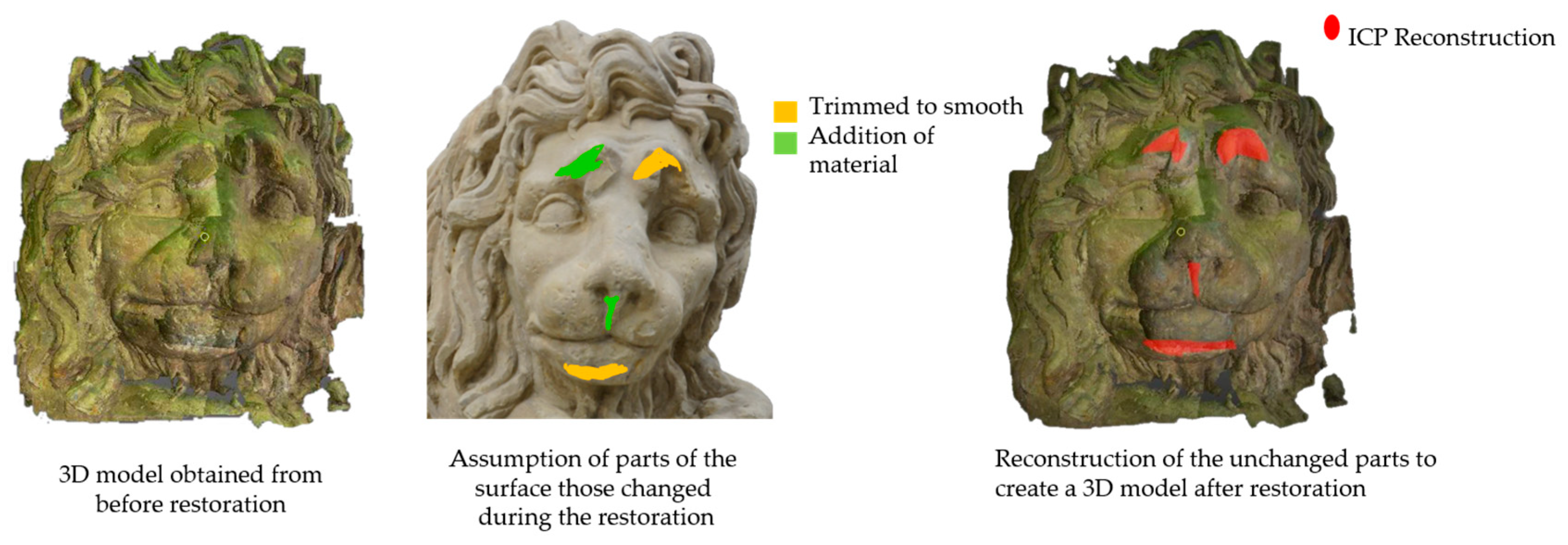
2.1. Reconstruction
2.1.1. Stitching of Point Clouds
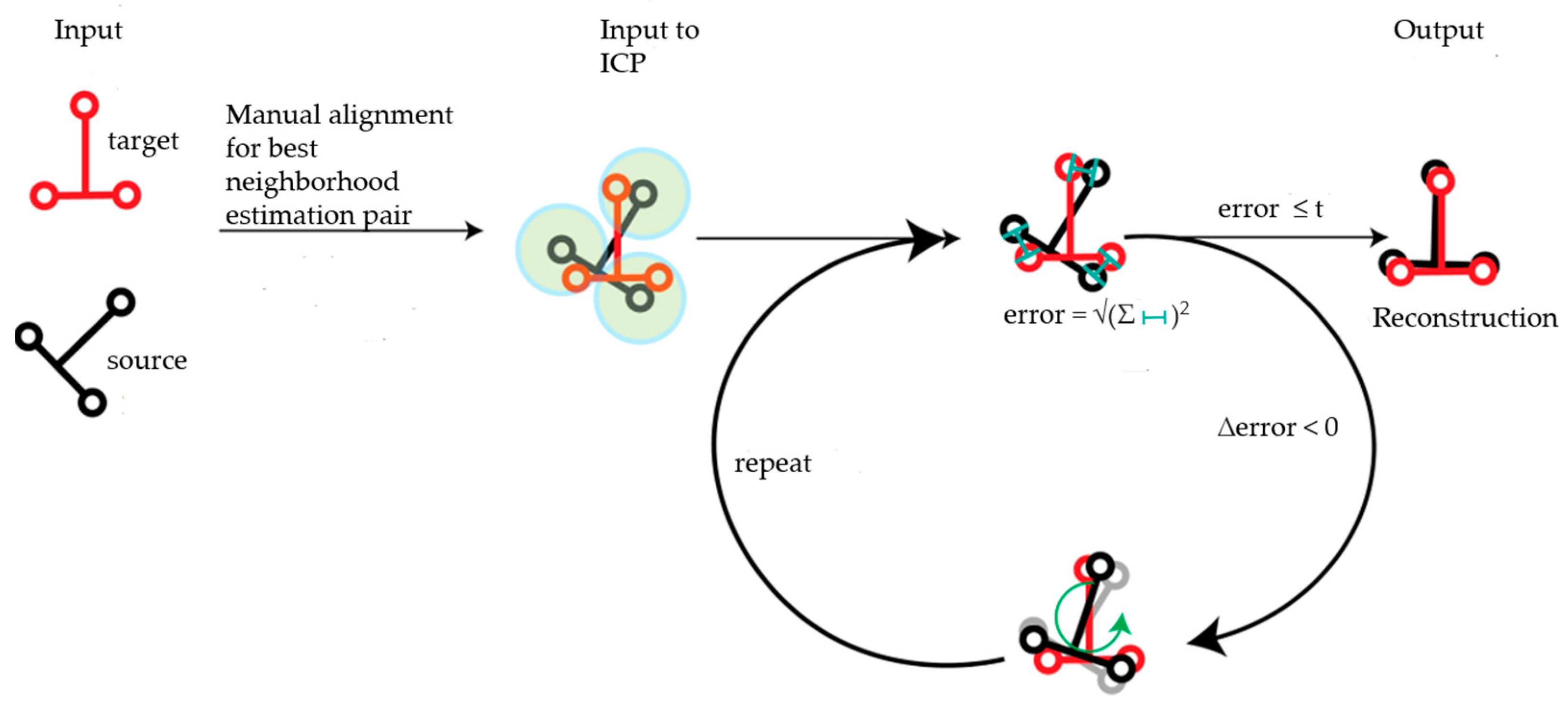
2.1.2. Cross-Time Alignment of the Models
2.2. Global Geometry Analysis
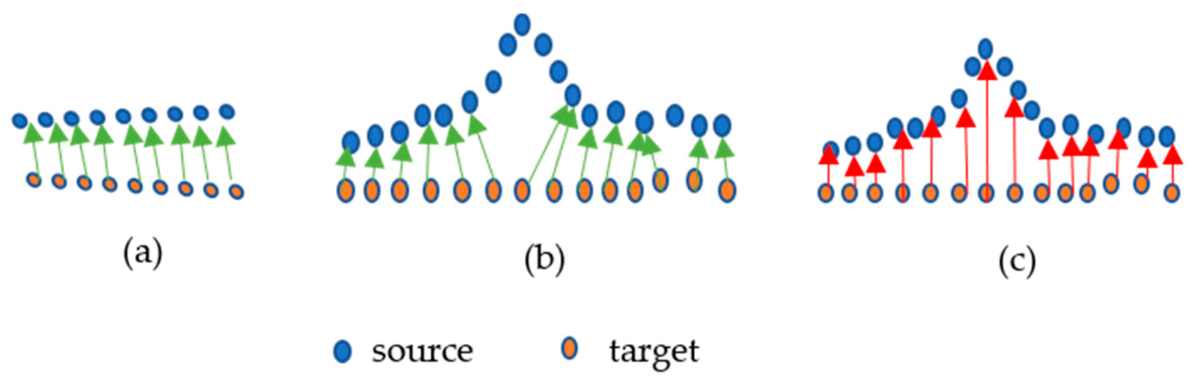
2.2.1. Point to Point Absolute Distance (P2P)
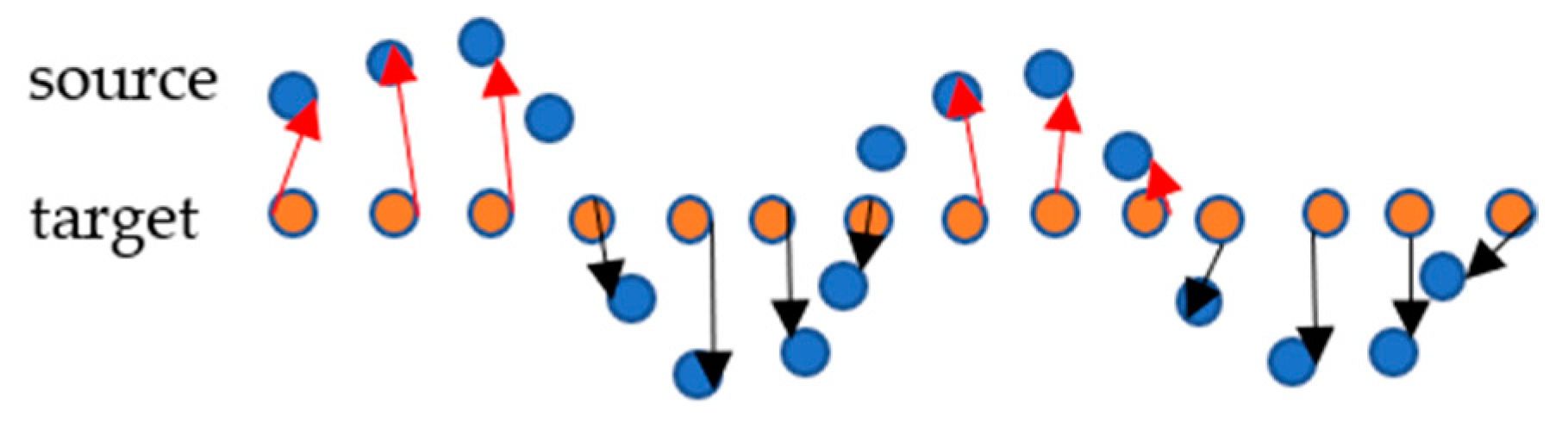
2.2.2. Point-to-Point Vector Distance (P2P_Direction)
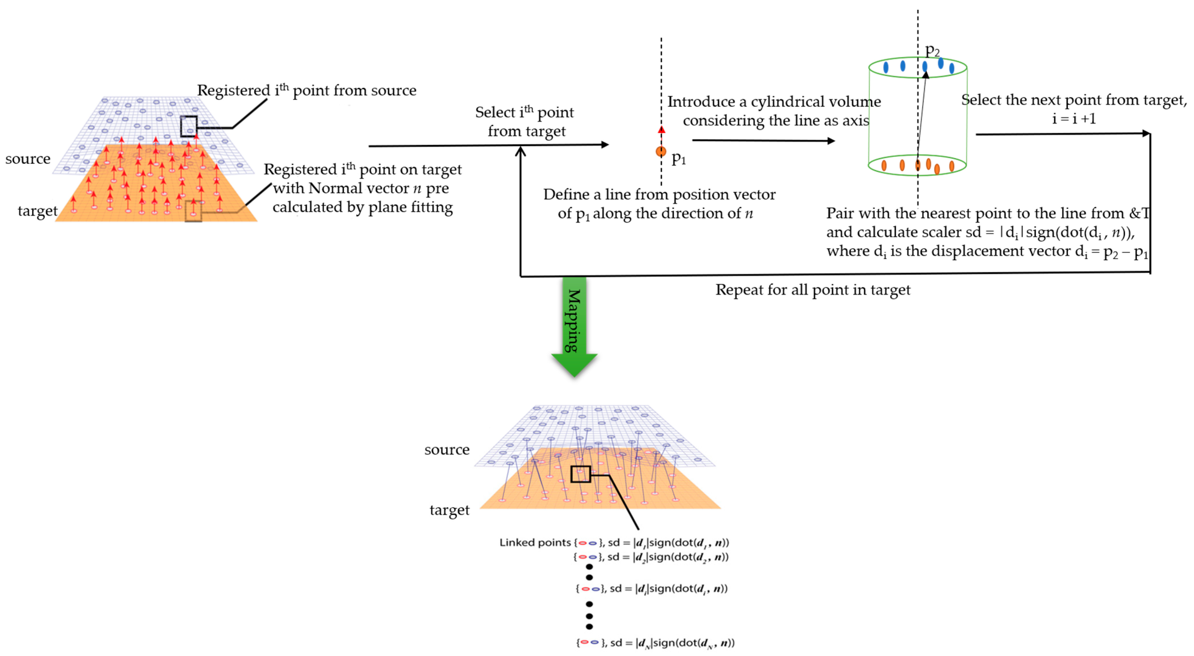
2.2.3. Point-to-Point along Normal Vector (P2P_AlongNV)
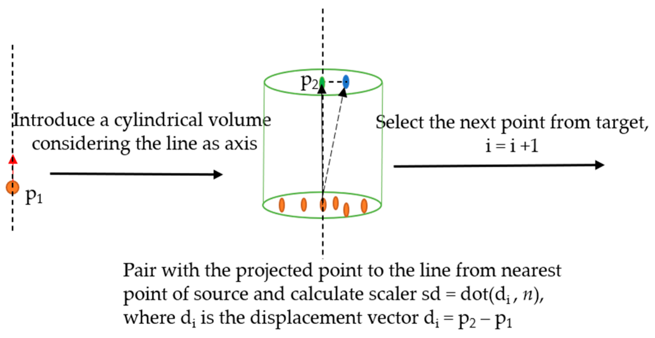
2.2.4. Point-To-Point Projection along Normal Vector (P2P_ProjectionAlongNV)
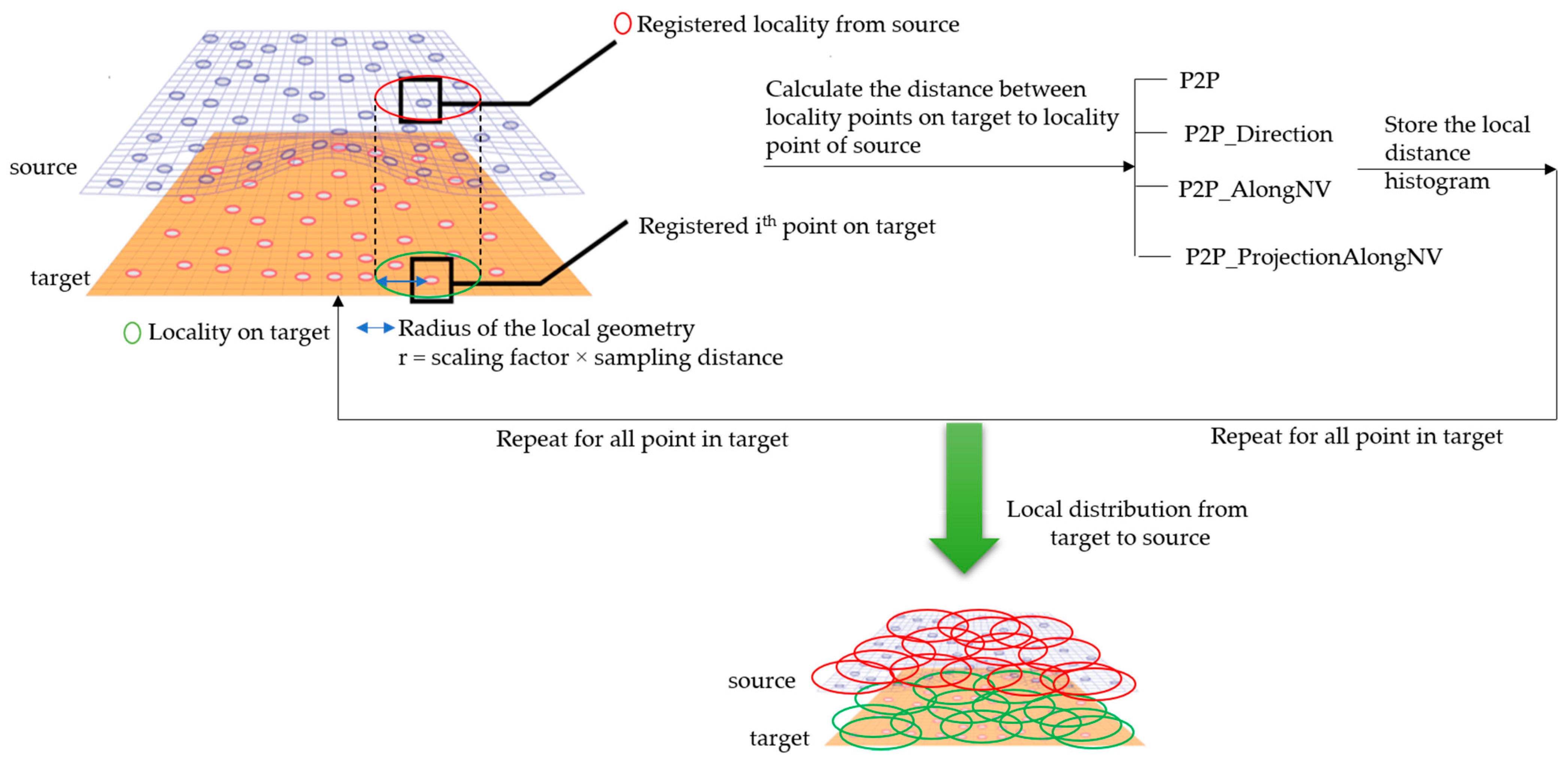
2.3. Local Geometry Analysis
2.4. Segmentation
2.5. Visualization
3. Results and Analysis
3.1. Case Study I
3.1.1. Results of Simulated Data
3.1.2. Results of Real Scenario
3.2. Case Study II
4. Conclusions
Author Contributions
Funding
Institutional Review Board Statement
Informed Consent Statement
Data Availability Statement
Acknowledgments
Conflicts of Interest
Appendix A


| Considered Stone Slabs for the Analysis | ||
|---|---|---|
| Stone Slabs | Material | Experiment |
| EL3 | Pentelic Marble | H2SO4 + HNO3(aq) Acid |
| ES1 | Pentelic Marble | H2SO4(aq) Acid |
| NGL2 | Grytdal Soapstone | Salt |
| NBL1 | Grytdal Soapstone | Freeze-Thaw |
| NBL2 | Grytdal Soapstone | Salt |
| NGS1 | Grytdal Soapstone | Outdoors/Trondheim |
| Stone Slabs | m1 (g) | m2 (g) | Δm (g) | Δm/m (%) |
|---|---|---|---|---|
| EL3 | 27.5131 | 27.4734 | −0.0397 | −0.14 |
| ES1 | 27.5872 | 27.5156 | −0.0716 | −0.26 |
| NGL2 | 160.5487 | 159.4037 | −1.1450 | −0.71 |
| NBL1 | 168.8975 | Unknown | ||
| NBL2 | 188.9025 | 179.8329 | −9.0696 | −4.80 |
| NGS1 | 20.6227 | 20.5998 | −0.0229 | −0.11 |
| Mean Erosion δ (mm) during Session 1 to Session 2 | ||||||
|---|---|---|---|---|---|---|
| Stone Slabs | V1 (cm3) | V2 (cm3) | ΔV (cm3) | S (cm2) | δ(a) (mm) | δ(b) (mm) |
| EL3 | 10.1391 | 10.1575 | 0.0184 | 29.7689 | 0.0065 | 0.0062 |
| ES1 | 10.1510 | 10.1497 | −0.0013 | 29.9718 | −0.0005 | −0.0004 |
| NGL2 | 55.2833 | 55.1410 | −0.1423 | 102.5810 | −0.0164 | −0.0139 |
| NBL1 | 61.7922 | Unknown | ||||
| NBL2 | 68.6979 | 66.6648 | −2.0331 | 125.6727 | −0.2040 | −0.1618 |
| NGS1 | 7.1294 | 7.1398 | 0.0104 | 24.6578 | 0.0047 | 0.0042 |
References
- Dante, A. Built-Heritage Multi-temporal Monitoring through Photogrammetry and 2D/3D Change Detection Algorithms. Stud. Conserv. 2019, 64, 423–434. [Google Scholar] [CrossRef]
- Logothetis, S.; Delinasiou, A.; Stylianidis, E. Building Information Modelling for Cultural Heritage: A review. ISPRS Ann. Photogramm. Remote. Sens. Spat. Inf. Sci. 2015, II-5/W3, 177–183. [Google Scholar] [CrossRef] [Green Version]
- Sitnik, R.; Lech, K.; Bunsch, E.; Michoński, J. Monitoring surface degradation process by 3D structured light scanning. In Proceedings of the SPIE 11058, Optics for Arts, Architecture, and Archaeology VII, Munich, Germany, 12 July 2019; p. 1105811. [Google Scholar] [CrossRef]
- Lague, D.; Brodu, N.; Leroux, J. Accurate 3D comparison of complex topography with terrestrial laser scanner: Application to the Rangitikei canyon (N-Z). ISPRS P&RS 2013, 82, 10–26. [Google Scholar] [CrossRef] [Green Version]
- Nicola, L. Monitoring earthen archaeological heritage using multi-temporal terrestrial laser scanning and surface change detection. J. Cult. Herit. 2019, 39, 152–165. [Google Scholar]
- Grilli, E.; Remondino, F. Classification of 3D Digital Heritage. Remote. Sens. 2019, 11, 847. [Google Scholar] [CrossRef] [Green Version]
- Murtiyoso, A.; Grussenmeyer, P. Automatic Heritage Building Point Cloud Segmentation and Classification Using Geometrical Rules. Int. Arch. Photogramm. Remote. Sens. Spat. Inf. Sci 2019, XLII-2/W15, 821–827. [Google Scholar] [CrossRef] [Green Version]
- Pérez-Sinticala, C.; Janvier, R.; Brunetaud, X.; Treuillet, S.; Aguilar, R.; Castañeda, B. Evaluation of Primitive Extraction Methods from Point Clouds of Cultural Heritage Buildings. In Structural Analysis of Historical Constructions. RILEM Bookseries; Aguilar, R., Torrealva, D., Moreira, S., Pando, M.A., Ramos, L.F., Eds.; Springer: Cham, Switzerland, 2019; Volume 18. [Google Scholar]
- Engelmann, F.; Kontogianni, T.; Schult, J.; Leibe, B. Know What Your Neighbors Do: 3D Semantic Segmentation of Point Clouds. In Computer Vision–ECCV 2018 Workshops. ECCV 2018. Lecture Notes in Computer Science; Leal-Taixé, L., Roth, S., Eds.; Springer: Cham, Switzerland, 2019; Volume 11131. [Google Scholar]
- Theologou, P.; Pratikakis, I.; Theoharis, T. Unsupervised Spectral Mesh Segmentation Driven by Heterogeneous Graphs. IEEE Trans. Pattern Anal. Mach. Intell. 2016, 39, 397–410. [Google Scholar] [CrossRef] [PubMed]
- Brezina, T.; Graser, A.; Leth, U. Geometric methods for estimating representative sidewalk widths applied to Vienna’s streetscape surfaces database. J. Geogr. Syst. 2017, 19, 157–174. [Google Scholar] [CrossRef] [Green Version]
- Sitnik, R.; Błaszczyk, P.M. Segmentation of unsorted cloud of points data from full field optical measurement for metrological validation. Comput. Ind. 2012, 63, 30–44. [Google Scholar] [CrossRef]
- Khatamian, A.; Hamid, A. Survey on 3D Surface Reconstruction. J. Inf. Process. Systems 2016, 12, 338–357. [Google Scholar] [CrossRef] [Green Version]
- Gupta, D.; Anand, R.S. A hybrid edge-based segmentation approach for ultrasound medical images. Biomed. Signal Process. Control. 2017, 31, 116–126. [Google Scholar] [CrossRef]
- Tchapmi, L.; Choy, C.; Armeni, I.; Gwak, J.; Savarese, S. Segcloud: Semantic Segmentation of 3D Point Clouds. In Proceedings of the 2017 International Conference on 3D Vision (3DV), Qingdao, China, 10–12 October 2017; pp. 537–547. [Google Scholar]
- Rethage, D.; Wald, J.; Sturm, J.; Navab, N.; Tombari, F. Fully Convolutional Point Networks for Large-Scale Point 765 Clouds. In Computer Vision–ECCV 2018; ECCV 2018. Lecture 766 Notes in Computer Science; Ferrari, V., Hebert, M., Sminchisescu, C., Weiss, Y., Eds.; Springer: Cham, Switzerland, 2018; Volume 11208. [Google Scholar]
- Haibin, H.; Evangelos, K.; Siddhartha, C.; Duygu, C.; Vladimir, G.K.; Ersin, Y. Learning Local Shape Descriptors from Part Correspondences with Multiview Convolutional Networks. ACM Trans. Graph. 2017, 37, 1–14. [Google Scholar] [CrossRef] [Green Version]
- Mączkowski, G.; Krzesłowski, J.; Sitnik, R. Integrated Method for Three-Dimensional Shape and Multispectral Color Measurement. J. Imaging Sci. Technol. 2011, 55, 30502-1–30502-10. [Google Scholar] [CrossRef]
- Tsakiri, M.; Vasileios-Athanasios, A. Change Detection in Terrestrial Laser Scanner Data via Point Cloud Correspondence. Int. J. Eng. Innov. Research 2015, 4, 476–486. [Google Scholar]
- He, Y.; Liang, B.; Yang, J.; Li, S.; He, J. An Iterative Closest Points Algorithm for Registration of 3D Laser Scanner Point Clouds with Geometric Features. Sensors 2017, 17, 1862. [Google Scholar] [CrossRef] [Green Version]
- Saha, S.; Duda-Maczuga, A.; Papanikolaou, A.; Sitnik, R. Approach for Identification of Geometry Change on Cultural Heritage Surface. In Proceedings of the IS&T International Symposium on Electronic Imaging 2021: 3D Imaging and Applications Proceedings, Online. San Francisco, CA, USA, 18 January 2021. [Google Scholar] [CrossRef]
- Saha, S.; Forys, P.; Martusewicz, J.; Sitnik, R. Approach to Analysis the Surface Geometry Change in Cultural Heritage Objects. In Proceedings of the ICISP 2020: 9th International Conference on Image and Signal Processing, Lecture Notes in Computer Science, Marrakesh, Morocco, 4–6 June 2020; Springer: Cham, Switzerland, 2020; Volume 12119. [Google Scholar] [CrossRef]
- Heidenreich, N.B.; Schindler, A.; Sperlich, S. Bandwidth selection for kernel density estimation: A review of fully automatic selectors. Adv. Stat. Analysis 2013, 97, 403–433. [Google Scholar] [CrossRef] [Green Version]
- Pilario, K.E.; Shafiee, M.; Cao, Y.; Lao, L.; Yang, S.-H. A Review of Kernel Methods for Feature Extraction in Nonlinear Process Monitoring. Processes 2020, 8, 24. [Google Scholar] [CrossRef] [Green Version]
- Wang, X.; Eric, P.; Daniel, X.; Schaid, J. Kernel methods for large-scale genomic data analysis. Brief. Bioinform. 2015, 16, 183–192. [Google Scholar] [CrossRef] [PubMed] [Green Version]
- Silverman, B.W. Density Estimation for Statistics and Data Analysis; Published in Monographs on Statistics and Applied Probability; Chapman and Hall: London, UK, 1986. [Google Scholar]
- Marcin, A.; Maciej, S.; Robert, S.; Adam, W. Hierarchical, Three-Dimensional Measurement System for Crime Scene Scanning. J. Forensic. Sci. 2017, 62, 889–899. [Google Scholar] [CrossRef]
- Theoharis, T.; Papaioannou, G. PRESIOUS 3D Cultural Heritage Fragments. 2013. Available online: http://presious.eu/resources/3d-data-sets (accessed on 14 May 2020).
- Michoński, J.; Witkowski, M.; Glinkowska, B.; Sitnik, R.; Glinkowski, W. Decreased Vertical Trunk Inclination Angle and Pelvic Inclination as the Result of Mid-High-Heeled Footwear on Static Posture Parameters in Asymptomatic Young Adult Women. Int. J. Environ. Res. Public Health 2019, 16, 4556. [Google Scholar] [CrossRef] [PubMed] [Green Version]
- Domasłowski, W. Preventive Conservation of Stone Historical Objects; Chapter 3: Causes of Stone Deterioration; Wydawnictwo Uniwersytetu Mikołaja Kopernika: Torun, Poland, 2003; ISBN 83-231-1645-8. [Google Scholar]


| Parameters | Unit | Description | Visual Paradigm |
|---|---|---|---|
| Sampling distance (sd) | Millimeter | The average point-to-point distance of the input data, i.e., resolution of the 3D scanner, is considered as the sampling distance. |  |
| Knn_Count (knn) | Integer | The total number of points, i.e., size of neighborhood inside each spherical neighborhood considered for the local geometry analysis, is termed Knn_Count. |  |
| Bandwidth (Bw) and Mean (mu) | Real | The bandwidth/number of bins that illustrate the appearance of the local distance histogram. The Bandwidth is calculated as in Equation (3). The mean of the histogram is the average of the values in the local distance histogram. Both the bandwidth and the mean are normalized to the resolution of the input data to make the segmentation method more independent of the input data. |  |
| Noise (N) | Real | The noise is basically calculated as the plane fitting error for the input data. The noise is calculated by using the random sampling of the input data. The randomly selected points were fitted to a best-fitting plane, considering the neighboring points up to a given radius of scaling factor × sd. The scaling factor for the analysis was set to 5; however, the user can scale it based on the density of the data. From randomly chosen points from the surface, the plane fitting error was calculated in terms of RMS distance from the considered points to the calculated plane. In this case, the noise was averaged from both the original and the changed surface. To make the method more independent of the resolution of the input data and the amount of noise, it was normalized with the calculated sampling distance. |  |
| Error 1 (e1) and Error 2 (e2) | Millimeter | From each locality and its corresponding local distribution, the plane error was calculated, and we inspected the behavior of those errors for the segmentation method. Both the original surface and the changed surface locality were considered for RMS distance calculation from the points to the local plane. However, this RMS distance calculation is confined to the local distribution, unlike the noise from the entire surface. |  |
| Threshold | Description |
|---|---|
| Deposit/Loss Threshold (Dt)/(Lt) | The deposit/loss threshold is used to define the amount of deposit/loss to/from the surface. This user input will quantify this as minor or major according to the change with respect to the size of the object. A deposit/loss less than the size of the deposit/loss threshold will be presented as minor while one greater than the threshold will be considered a major deposit/loss on the surface. |
| Nonchanged Threshold (Nt) | This threshold was considered based on the alignment of the 3D models and the accuracy. The alignment threshold is a ratio of normalized noise, for which a default value is set to 1. However, the user can increase the value in certain cases with known reference to an unchanged part of the surface. In some cases, based on user expertise of the object material and the considered time interval, an unchanged threshold can be set to a particular value that will provide more accuracy for the quantification of changes. |
| Change Types | Local Naming | Parameter’s Behavior |
|---|---|---|
| Type 1 | No Change | |
| Type 2 | Minor Change (Deposit)
|
|
Minor Change (Loss)
|
| |
| Type 3 | Major Change (Deposit)
|
|
Major Change (Loss)
|
| |
| Type 4 | Unknown | Other behavior of parameters. |
| Change Types | Assigned Code | Assigned RGB Code/Color | ||
|---|---|---|---|---|
| Type 1 | 0 | (0, 0, 255)  | ||
| Type 2 | +1 (Deposit) | (0, 128, 255)  Equal | (0, 255, 255)  Linear | (153, 255, 255)  Non-linear |
| −1 (Loss) | (255, 255, 153)  Equal | (255, 255, 0)  Linear | (255, 128, 0)  Non-linear | |
| Type 3 | +2 (Deposit) | (153, 255, 153)  Equal | (0, 255, 0)  Linear | (0, 102, 0)  Non-linear |
| −2 (Loss) | (255, 102, 102)  Equal | (255, 0, 0)  Linear | (153, 0, 0)  Non-linear | |
| Type 4 | X | (102, 0, 0)  | ||
| Datasets | N (mm) | sd (mm) | Normalized Noise N/sd | Nt (Scaled by N/sd) | Dt (mm) | Lt (mm) |
|---|---|---|---|---|---|---|
| Simulated data | 0.015 | 0.098 | 0.15 | 1 | 1 | 1 |
| Real scenario | 0.014 | 0.010 | 0.14 | 100 | 0.5 | 2 |
| Method | Global Geometry Analysis | Segmentation |
|---|---|---|
| P2P |  |  |
| P2P_Direction |  |  |
| P2P_AlongNV |  |  |
| P2P_ProjectionAlongNV |  |  |
| Method | Global Geometry Analysis | Segmentation |
|---|---|---|
| P2P |  |  |
| P2P_Direction |  |  |
| P2P_AlongNV |  |  |
| P2P_ProjectionAlongNV |  |  |
| Considered Stone Slabs for the Analysis and Monitoring Period | ||
|---|---|---|
| Stone Slabs (Naming from [30]) | Session 1 | Session 2 |
| Elefsis Large 03(EL3) | 2015-01-12 | 2015-05-15 |
| Elefsis Small 01 (ES1) | 2015-01-12 | 2015-05-15 |
| Nidaros Good Large 02 (NGL2) | 2015-01-12 | 2015-05-15 |
| Nidaros Bad Large 01 (NBL1) | 2015-01-12 | 2015-12-04 |
| Nidaros Bad Large 02 (NBL2) | 2015-01-12 | 2015-05-15 |
| Nidaros Good Small 01 (NGS1) | 2015-01-12 | 2015-05-15 |
| Stone Slabs | Original Surface | Changed Surface |
|---|---|---|
| Session 1 | Session 2 | |
| EL3 |  |  |
| ES1 |  |  |
| NGL2 |  |  |
| NBL1 |  |  |
| NBL2 |  |  |
| NGS1 |  |  |
| Datasets | N (mm) | sd (mm) | Normalized Noise N/s | Nt (Scaled by N/s) | Dt (mm) | Lt (mm) |
|---|---|---|---|---|---|---|
| EL3 | 0.006 | 0.072 | 0.09 | 1 | 0.1 | 0.2 |
| ES1 | 0.006 | 0.072 | 0.08 | 0.1 | 0.2 | |
| NGL2 | 0.007 | 0.062 | 0.10 | 0.15 | 0.5 | |
| NBL1 | 0.007 | 0.056 | 0.12 | 0.25 | 1 | |
| NBL2 | 0.008 | 0.065 | 0.12 | 0.25 | 1 | |
| NGS1 | 0.008 | 0.070 | 0.11 | 0.15 | 0.5 |
| Method | P2P | P2P_Direction | P2P_AlongNV | P2P_ProjectionAlongNV |
|---|---|---|---|---|
| Global Geometry Analysis |  |  |  |  |
| Segmentation |  |  |  |  |
| Segmentation | Total Point Count | No Change | Minor Change | Major Change | % of Surface with Deposit | % of Surface with Loss | ||
|---|---|---|---|---|---|---|---|---|
| Deposit | Loss | Deposit | Loss | |||||
| P2P_Direction | 976,587 | 1 | 363,788 | 496,653 | 13,368 | 115,978 | 37.25 | 62.74 |
| P2P_AlongNV | 1 | 261,220 | 393,974 | 4464 | 316,928 | 27.20 | 72.80 | |
| P2P_ProjectionAlongNV | 557 | 267,661 | 407,043 | 5768 | 295,558 | 27.01 | 72.95 | |
| Method | P2P | P2P_Direction | P2P_AlongNV | P2P_ProjectionAlongNV |
|---|---|---|---|---|
| Global Geometry Analysis |  |  |  |  |
| Segmentation |  |  |  |  |
| Segmentation | Total Point Count | No Change | Minor Change | Major Change | % of Surface with Deposit | % of Surface with Loss | ||
|---|---|---|---|---|---|---|---|---|
| Deposit | Loss | Deposit | Loss | |||||
| P2P_Direction | 854,730 | 0 | 286,411 | 473,175 | 73,094 | 22,050 | 42.06 | 57.94 |
| P2P_AlongNV | 0 | 159,543 | 310,138 | 159,421 | 225,628 | 37.31 | 62.69 | |
| P2P_ProjectionAlongNV | 5 | 299,863 | 50,2268 | 16,905 | 35,689 | 37.06 | 62.94 | |
| Method | P2P | P2P_Direction | P2P_AlongNV | P2P_ProjectionAlongNV |
|---|---|---|---|---|
| Global Geometry Analysis |  |  |  |  |
| Segmentation |  |  |  |  |
| Segmentation | Total Point Count | No Change | Minor Change | Major Change | % of Surface with Deposit | % of Surface with Loss | ||
|---|---|---|---|---|---|---|---|---|
| Deposit | Loss | Deposit | Loss | |||||
| P2P_Direction | 3,545,412 | 11 | 1,792,619 | 1,587,970 | 97,467 | 67,345 | 53.32 | 46.69 |
| P2P_AlongNV | 22 | 1,817,344 | 1,426,692 | 14,482 | 286,872 | 51.67 | 48.33 | |
| P2P_ProjectionAlongNV | 872 | 1,828,897 | 1,437,406 | 15,926 | 262,311 | 52.03 | 47.98 | |
| Method | P2P | P2P_Direction | P2P_AlongNV | P2P_ProjectionAlongNV |
|---|---|---|---|---|
| Global Geometry Analysis |  |  |  |  |
| Segmentation |  |  |  |  |
| Segmentation | Total Point Count | No Change | Minor Change | Major Change | % of Surface with Deposit | % of Surface with Loss | ||
|---|---|---|---|---|---|---|---|---|
| Deposit | Loss | Deposit | Loss | |||||
| P2P_Direction | 2,671,989 | 135 | 924,015 | 1,337,342 | 122,829 | 287,667 | 39.17 | 60.82 |
| P2P_AlongNV | 138 | 870,475 | 1,309,608 | 10,023 | 481,745 | 32.95 | 67.04 | |
| P2P_ProjectionAlongNV | 2083 | 860,933 | 1,376,565 | 12,852 | 419,556 | 32.70 | 67.22 | |
| Method | P2P | P2P_Direction | P2P_AlongNV | P2P_ProjectionAlongNV |
|---|---|---|---|---|
| Global Geometry Analysis |  |  |  |  |
| Segmentation |  |  |  |  |
| Segmentation | Total Point Count | No Change | Minor Change | Major Change | % of Surface with Deposit | % of Surface with Loss | ||
|---|---|---|---|---|---|---|---|---|
| Deposit | Loss | Deposit | Loss | |||||
| P2P_Direction | 3,978,584 | 3 | 1,502,188 | 1,780,675 | 229,699 | 466,019 | 43.53 | 56.46 |
| P2P_AlongNV | 3 | 1,607,029 | 1,542,373 | 6891 | 822,280 | 40.57 | 59.43 | |
| P2P_ProjectionAlongNV | 161 | 1,802,635 | 1,595,841 | 5951 | 573,996 | 45.46 | 54.53 | |
| Method | P2P | P2P_Direction | P2P_AlongNV | P2P_ProjectionAlongNV |
|---|---|---|---|---|
| Global Geometry Analysis |  |  |  |  |
| Segmentation |  |  |  |  |
| Segmentation | Total Point Count | No Change | Minor Change | Major Change | % of Surface with Deposit | %of Surface with Loss | ||
|---|---|---|---|---|---|---|---|---|
| Deposit | Loss | Deposit | Loss | |||||
| P2P_Direction | 600,857 | 38 | 242,324 | 349,888 | 3677 | 4930 | 40.94 | 59.05 |
| P2P_AlongNV | 42 | 200,138 | 370,322 | 8787 | 21,568 | 34.78 | 65.22 | |
| P2P_ProjectionAlongNV | 1218 | 201,266 | 369,771 | 8974 | 19,628 | 34.99 | 64.80 | |
Publisher’s Note: MDPI stays neutral with regard to jurisdictional claims in published maps and institutional affiliations. |
© 2021 by the authors. Licensee MDPI, Basel, Switzerland. This article is an open access article distributed under the terms and conditions of the Creative Commons Attribution (CC BY) license (https://creativecommons.org/licenses/by/4.0/).
Share and Cite
Saha, S.; Martusewicz, J.; Streeton, N.L.W.; Sitnik, R. Segmentation of Change in Surface Geometry Analysis for Cultural Heritage Applications. Sensors 2021, 21, 4899. https://doi.org/10.3390/s21144899
Saha S, Martusewicz J, Streeton NLW, Sitnik R. Segmentation of Change in Surface Geometry Analysis for Cultural Heritage Applications. Sensors. 2021; 21(14):4899. https://doi.org/10.3390/s21144899
Chicago/Turabian StyleSaha, Sunita, Jacek Martusewicz, Noëlle L. W. Streeton, and Robert Sitnik. 2021. "Segmentation of Change in Surface Geometry Analysis for Cultural Heritage Applications" Sensors 21, no. 14: 4899. https://doi.org/10.3390/s21144899
APA StyleSaha, S., Martusewicz, J., Streeton, N. L. W., & Sitnik, R. (2021). Segmentation of Change in Surface Geometry Analysis for Cultural Heritage Applications. Sensors, 21(14), 4899. https://doi.org/10.3390/s21144899