Figure 1.
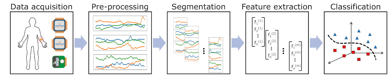
Pattern recognition chain including several steps that should be optimised in parallel to yield the best performance.
Figure 1.
Pattern recognition chain including several steps that should be optimised in parallel to yield the best performance.
Figure 2.
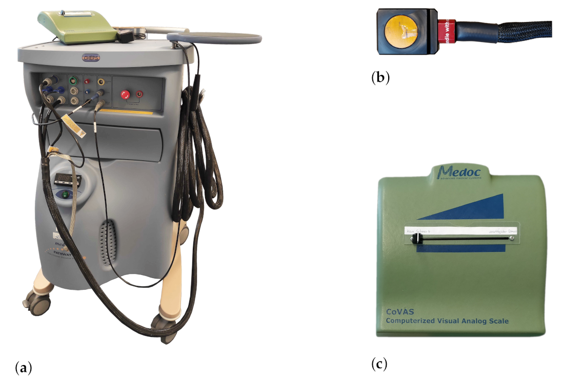
The Medoc devices used during data acquisition. (a) Medoc Pathway system. (b) Cheps thermode.(c) Computerised Visual Analogue Scale (CoVAS) slider.
Figure 2.
The Medoc devices used during data acquisition. (a) Medoc Pathway system. (b) Cheps thermode.(c) Computerised Visual Analogue Scale (CoVAS) slider.
Figure 3.
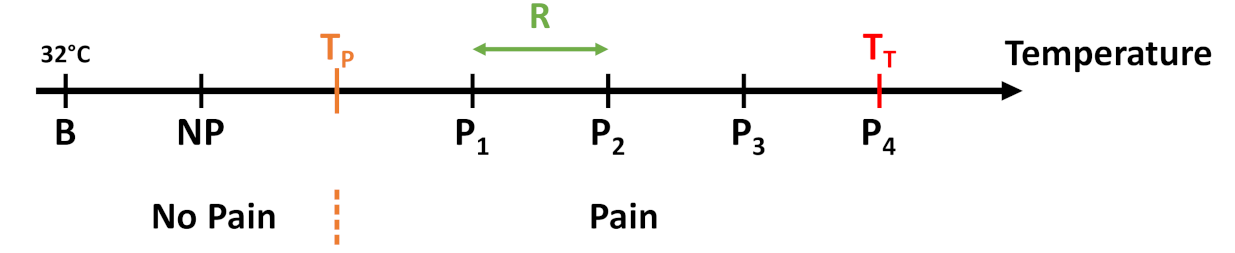
The 5 temperature intervals defined by the temperature range R in dependency of and . While the first temperature resembles a non-painful stimulus, the last 4 are meant to evoke pain.
Figure 3.
The 5 temperature intervals defined by the temperature range R in dependency of and . While the first temperature resembles a non-painful stimulus, the last 4 are meant to evoke pain.
Figure 4.
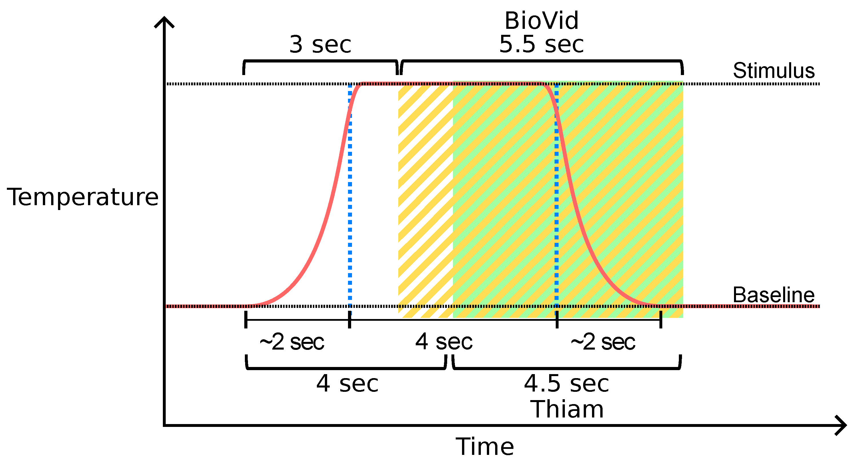
Window segmentation of the BioVid Heat Pain Database (BVDB) dataset. Window segments available in the public BVDB are highlighted in yellow. Thiam et al. [
38] proposed another segmentation process highlighted in green that is used in [
30,
33] as well.
Figure 4.
Window segmentation of the BioVid Heat Pain Database (BVDB) dataset. Window segments available in the public BVDB are highlighted in yellow. Thiam et al. [
38] proposed another segmentation process highlighted in green that is used in [
30,
33] as well.
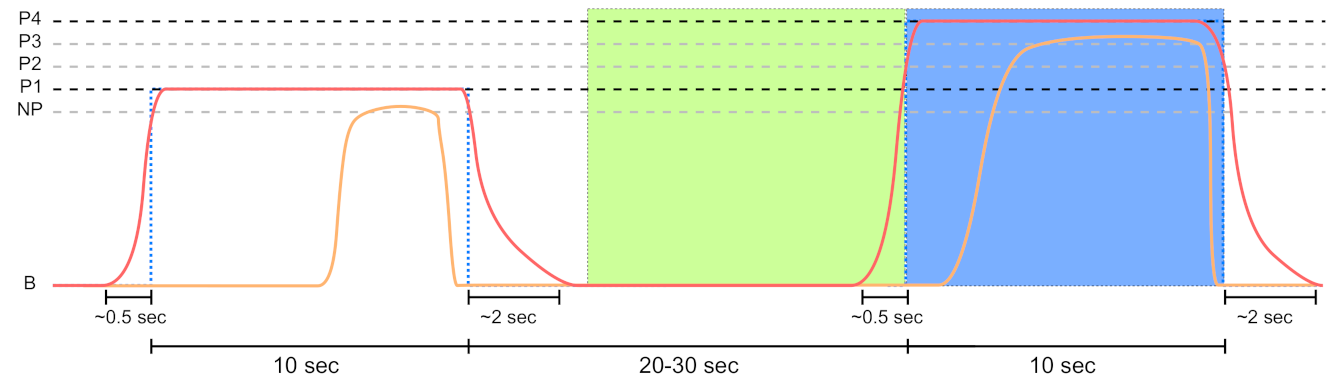
Figure 5.
Sensor data segmentation of 10 s non-painful (green area) and painful (blue area) windows for the PainMonit Database (PMDB). The windows are centred around the on and offsets of the temperature (red curve) stimulus. Moreover, the CoVAS (orange curve) values are used to create a pain label that incorporates the subjective sensation of the subjects.
Figure 6.
Electrodermal Activity (EDA) decomposition into the phasic and tonic signal with galvanic skin response detection. (a) The filtered input and retrieved tonic signal. (b) The phasic component with possible on- and offset for the peaks. (c) The raw signal with Skin Conductance Response (SCR) and their associated peaks, half recovery, on- and offsets.
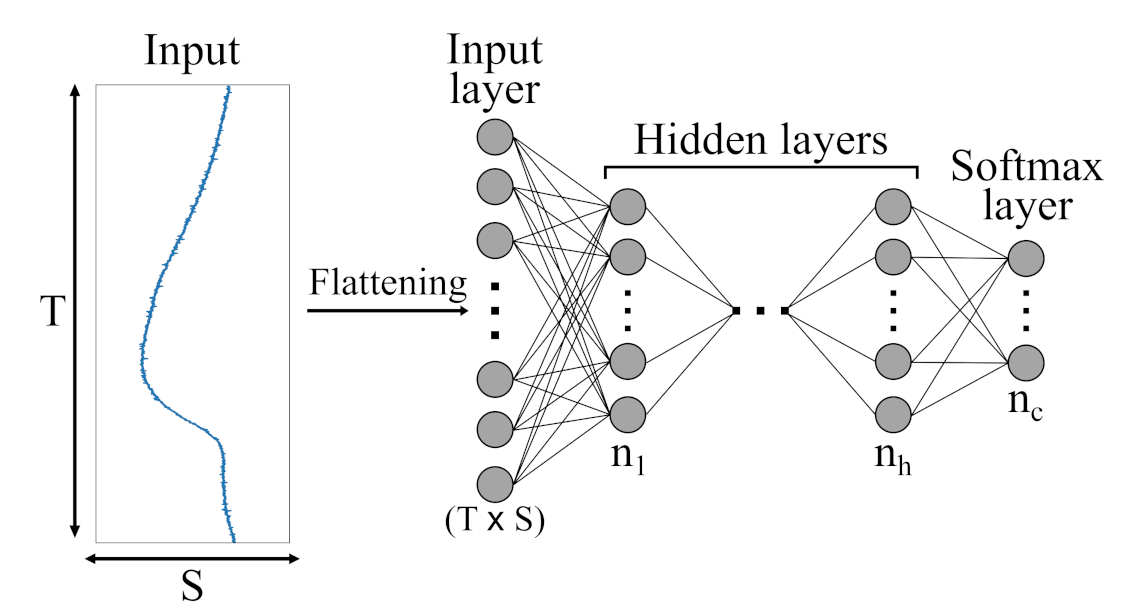
Figure 7.
Schematic illustration of an Multi-Layer Perceptron (MLP) architecture with h hidden layers and c output classes presented by a softmax layer. Initially, the different sensor channels are flattened into a ()-dimensional vector and then fed to the various hidden layers.
Figure 7.
Schematic illustration of an Multi-Layer Perceptron (MLP) architecture with h hidden layers and c output classes presented by a softmax layer. Initially, the different sensor channels are flattened into a ()-dimensional vector and then fed to the various hidden layers.
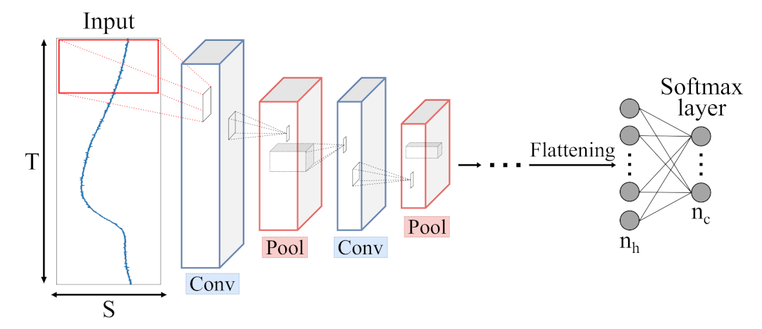
Figure 8.
Schematic illustration of a Convolutional Neural Network (CNN) architecture with c output classes presented by a softmax layer. Input data is processed by Convolutional (blue) and Pooling (red) layers, extracting meaningful features which are fed to a combination of dense layers, similar to single MLP layers.
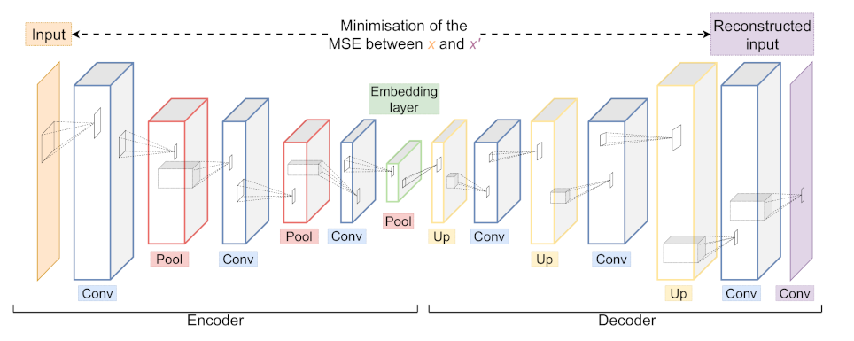
Figure 9.
An example of a Convolutional Autoencoder (CAE) architecture with its Encoder and Decoder part consisting of Convolutional (blue), Pooling (red) and Upsampling (yellow) layers. During training, the network is optimised to minimise the difference between input x and output . The embedding layer (green) yields a low dimensional representation of the input x.
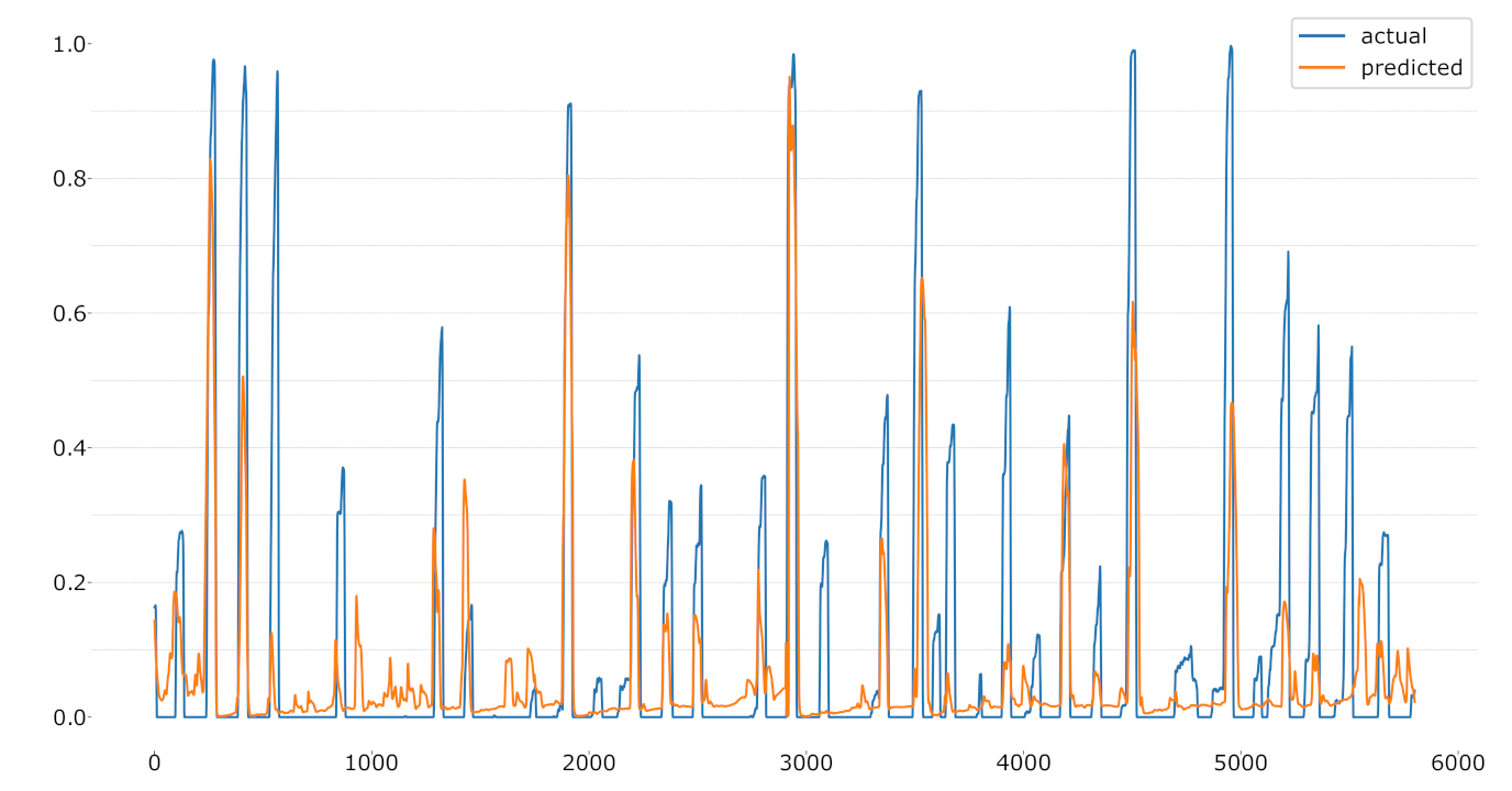
Figure 10.
LOSO regression using the CoVAS values as label.
Figure 10.
LOSO regression using the CoVAS values as label.
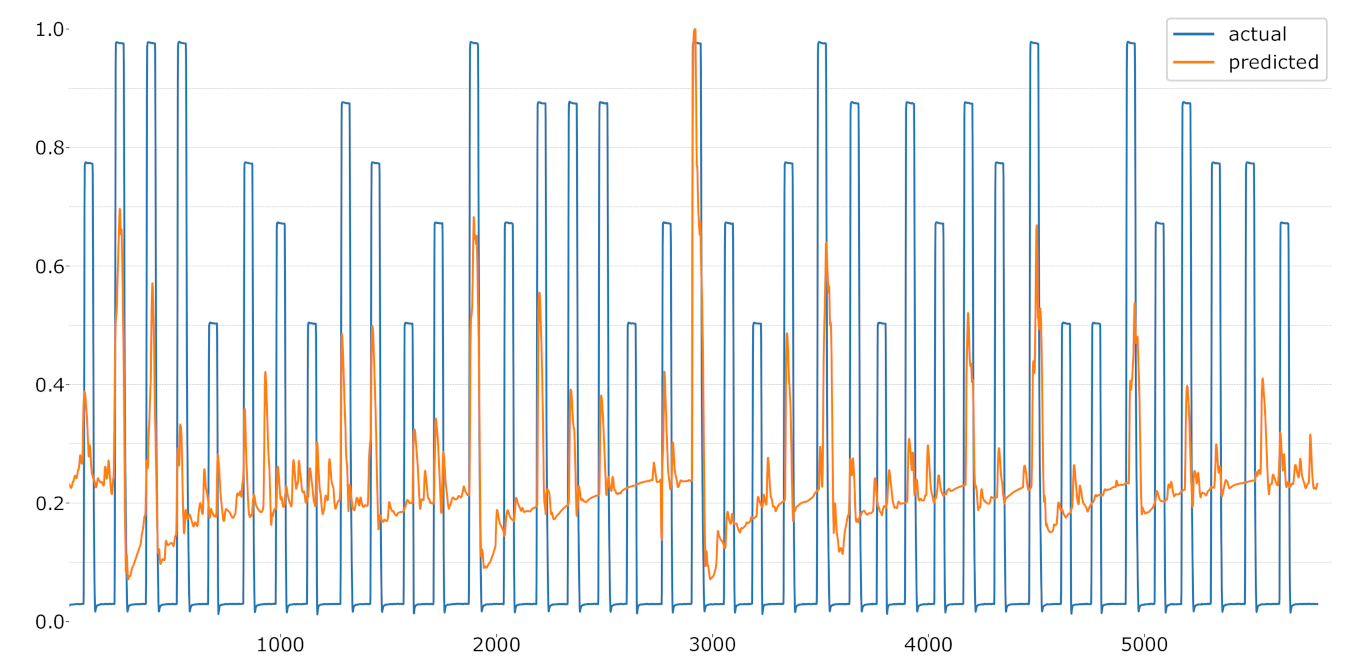
Figure 11.
LOSO regression using the temperature values as label.
Figure 11.
LOSO regression using the temperature values as label.
Table 1.
Features computed for the EDA signal.
Table 1.
Features computed for the EDA signal.
| Features |
|---|
| root mean square (RMS) |
| mean value of local maxima & minima |
| mean absolute value |
| mean of the absolute values (mav) of the first differences (mavfd) |
| mavfd on standardised signal |
| mav of the second differences (mavsd) |
| mavsd on standardised signal |
| variation of the first and second moment |
| indices of the minimum & maximum values; difference first and last value |
| mean & Standard Deviation (STD) for phasic, tonic, amplitudes, |
| rise times half recovery and recovery range of tonic; number of |
| Galvanic Skin Response (GSRs); sum of amplitudes; first amplitude; phasic max; |
| mean, STD and Variance (VAR) on normalised signal |
Table 2.
MLP architecture.
Table 2.
MLP architecture.
| Layer Name | Neurons/Drop Rate | Activation |
|---|
| Flatten | - | - |
| Dropout | 0.1 | - |
| Dense | 250 | - |
| Dropout | 0.1 | - |
| Dense | 100 | - |
| Dense | 2 | Softmax |
Table 3.
CNN architecture with dropout rate set to 0.1.
Table 3.
CNN architecture with dropout rate set to 0.1.
| Layer Name | No. Kernels (Units) | Kernel (Pool) Size | Stride | Activation |
|---|
| Convolutional | 16 | 7 | 2 | ReLU |
| Max Pooling | - | 4 | - | - |
| Dropout | - | - | - | - |
| Convolutional | 16 | 7 | 2 | ReLU |
| Max Pooling | - | 4 | - | - |
| Dropout | - | - | - | - |
| Flatten | - | - | - | - |
| Dense | 100 | - | - | - |
| Dense | 2 | - | - | Softmax |
Table 4.
The architecture that uses ConvLSTM blocks, later referred to as just ’LSTM’ with a drop rate set to 0.1. The ’return_sequences’ parameter for the ConvLSTM layers was set to True.
Table 4.
The architecture that uses ConvLSTM blocks, later referred to as just ’LSTM’ with a drop rate set to 0.1. The ’return_sequences’ parameter for the ConvLSTM layers was set to True.
| Layer Name | No. Kernels (Units) | Kernel (Pool) Size | Stride | Activation | Recurrent
Activation |
|---|
| ConvLSTM2D | 32 | 11 | 8 | Tanh | Hard sigmoid |
| Dropout | - | - | - | - | - |
| Batch normalisation | - | - | - | - | - |
| Max Pooling (3D) | - | 4 | - | - | - |
| ConvLSTM2D | 16 | 7 | 8 | - | Hard sigmoid |
| Dropout | - | - | - | - | - |
| Batch normalisation | - | - | - | - | - |
| Max Pooling (3D) | - | 4 | - | - | - |
| ConvLSTM2D | 8 | 3 | 2 | - | Hard sigmoid |
| Dropout | - | - | - | - | - |
| Batch normalisation | - | - | - | - | - |
| Max Pooling (3D) | - | 4 | - | - | - |
| Flatten | - | - | - | - | - |
| Dropout | - | - | - | - | - |
| Dense | 100 | - | - | ReLU | - |
| Dense | 2 | - | - | Softmax | - |
Table 5.
CAE architecture with its encoder and decoder part.
Table 5.
CAE architecture with its encoder and decoder part.
| Layer Name | No. Kernels (Units) | Kernel (Pool) Size |
|---|
| Convolutional | 64 | 7 |
| Max Pooling | - | 4 |
| Convolutional | 32 | 11 |
| Max Pooling | - | 4 |
| Convolutional | 16 | 11 |
| Max Pooling | - | 4 |
| Up Sampling | - | 4 |
| Convolutional | 16 | 11 |
| Up Sampling | - | 4 |
| Convolutional | 32 | 11 |
| Up Sampling | - | 4 |
| Convolutional | 64 | 7 |
| Convolutional | 1 | 1 |
Table 6.
Leave-one-subject-out (LOSO) average performance using the EDA sensor of the BVDB for several feature extraction methods in combination with a Random Forest. Performance metrics are given as average accuracy (upper) and (lower half) ± average standard deviation of each individual LOSO run. The best performing approach is highlighted in grey. Moreover, a paired student’s t-test with a significance level of 5% was performed to check the significance in differences between the accuracies obtained by each pair of approaches for each classification problem. indicate a significant improvement compared to the HCF, dPhEDA, TVSymp, MTVSymp, “HCF combined”, MLP, CNN, LSTM, and CAE approaches, respectively.
| Method | vs. | vs. | vs. | vs. |
|---|
| | HCF | | | | |
| | dPhEDA | | | | |
| | TVSymp | | | | |
| | MTVSymp | | | | |
| Acc | HCF combined | | | | |
| | MLP | | 64.68 ± 14.06 1,2,3,4,5,7,8 | 74.77 ± 13.79 2,3,4,5,7,8 | 84.01 ± 14.01 1,2,3,4,5,7,8 |
| | CNN | | | | |
| | LSTM | | | | |
| | CAE | 58.39 ± 12.31 2,3,4,7,8 | | | |
| | HCF | | | | |
| | dPhEDA | | | | |
| | TVSymp | | | | |
| | MTVSymp | | | | |
| HCF combined | | | | |
| | MLP | | 63.47 ± 15.10 | 73.96 ± 14.68 | 83.58 ± 14.78 |
| | CNN | | | | |
| | LSTM | | | | |
| | CAE | 57.77 ± 12.59 2,3,4,7,8 | | | |
Table 7.
LOSO accuracy performance comparison to early work on the EDA signal of the BVDB. The best performing approach is highlighted in grey.
Table 7.
LOSO accuracy performance comparison to early work on the EDA signal of the BVDB. The best performing approach is highlighted in grey.
| Method | vs. | vs. | vs. | vs. |
|---|
| Werner et al. [31] | 55.40 | 60.20 | 65.90 | 73.80 |
| Lopez-Martinez et al. [56] | 56.44 | 59.40 | 66.00 | 74.21 |
| Thiam et al. [30] | 61.67 ± 12.54 | 66.93 ± 16.19 | 76.38 ± 14.70 | 84.57 ± 14.13 |
| MLP (Ours) | | | | |
Table 8.
LOSO average performance using different EDA sensor combinations of the PMDB with an MLP + Random Forest (RF) classifier. The best performing approach is highlighted in grey. Moreover, a paired student’s t-test with a significance level of 5% was performed to check the significance in differences between the accuracies obtained by each pair of approaches for each classification problem. indicate a significant improvement compared to the EDA_RB, EDA_E4, and fusion approaches, respectively.
| Method | B vs. | B vs. | B vs. | B vs. | B vs. |
|---|
| EDA_RB | | | | 72.84 ± 14.27 2,3 | 86.50 ± 12.76 2,3 |
| Acc | EDA_E4 | | | | | |
| | Both | 54.59 ± 12.97 1,2 | 58.37 ± 13.39 2 | 64.59 ± 13.60 1,2 | | |
| EDA_RB | | 56.12 ± 11.49 | 61.86 ± 13.25 | 71.57 ± 15.37 | 85.82 ± 13.98 |
| EDA_E4 | 49.79 ± 14.46 | | | | |
| | Both | | | | | |
Table 9.
LOSO average performance using the EDA (RespiBan) sensor of the PMDB for several feature extraction methods in combination with a Random Forest. Performance metrics are given as average accuracy (upper) and (lower half) ± standard deviation. The best performing approach is highlighted in grey. Moreover, a paired student’s t-test with a significance level of 5% was performed to check the significance in differences between the accuracies obtained by each pair of approaches for each classification problem. indicate a significant improvement compared to the HCF, dPhEDA, TVSymp, MTVSymp, “HCF combined”, MLP, CNN, LSTM, and CAE approaches, respectively.
| Method | B vs. | B vs. | B vs. | B vs. | B vs. |
|---|
| HCF | 51.61 ± 12.51 2,3,4,5,7,8,9 | | | 73.99 ± 13.02 2,3,4,5,7,8,9 | |
| | dPhEDA | | | | | |
| | TVSymp | | | | | |
| | MTVSymp | | | | | |
| Acc | HCF combined | | | | | |
| | MLP | | | | | |
| | CNN | | 58.08 ± 11.08 3,4,8 | | | 87.41 ± 11.99 2,3,4,5,6 |
| | LSTM | | | | | |
| | CAE | | | 64.75 ± 12.70 1,2,3,4,6,8 | | |
| HCF | 50.43 ± 12.70 | | | 72.33 ± 14.79 | |
| | dPhEDA | | | | | |
| | TVSymp | | | | | |
| | MTVSymp | | | | | |
| HCF combined | | 55.68 ± 10.47 | 62.97 ± 13.75 | | |
| | MLP | | | | | |
| | CNN | | 56.39 ± 11.62 | | | 86.70 ± 13.41 |
| | LSTM | | | | | |
| | CAE | | | 63.46 ± 13.46 | | |
Table 10.
LOSO average performance using the EDA (RespiBan) sensor of the PMDB for several feature extraction methods in combination with a Random Forest. In contrast to previous tables, the CoVAS parameters are used as label here. Performance metrics are given as average accuracy (upper) and (lower half) ± standard deviation. The best performing approach is highlighted in grey. Moreover, a paired student’s t-test with a significance level of 5% was performed to check the significance in differences between the accuracies obtained by each pair of approaches for each classification problem. indicate a significant improvement compared to the HCF, dPhEDA, TVSymp, MTVSymp, “HCF combined”, MLP, CNN, LSTM, and CAE approaches, respectively.
| Method | vs. | vs. | vs. | vs. |
|---|
| HCF | | | 88.73 ± 08.05 2,3,4,7,8,9 | 93.78 ± 06.43 2,3,4,7,8 |
| | dPhEDA | | | | |
| | TVSymp | | | | |
| | MTVSymp | | | | |
| Acc | HCF combined | | | | |
| | MLP | 66.47 ± 09.39 2,3,4,7,9 | | | |
| | CNN | | | | |
| | LSTM | | | | |
| | CAE | | 83.10 ± 08.91 2,3,4,8 | | |
| HCF | | | 79.09 ± 15.53 | 87.60 ± 13.48 |
| | dPhEDA | | | | |
| | TVSymp | | | | |
| | MTVSymp | | | | |
| HCF combined | | | | |
| | MLP | 58.54 ± 10.84 | | | |
| | CNN | | | | |
| | LSTM | | | | |
| | CAE | | 68.62 ± 15.97 | | |


 ,
, 


