
Single-Camera-Based Bridge Structural Displacement Measurement with Traffic Counting


Abstract
:1. Introduction
- Primary effects—related to the bridge’s material, construction type, shape, and design considerations in relation to the bridge’s expected load and its dead weight under static condition.
- Secondary effects—identified from the time-bound dynamic structural response excited from forcing actions due to vehicular loads, wind, quake, or thermal expansion/shrinkage, which are often nonlinear and inelastic.
- Tertiary effects—not directly related to static nor dynamic properties of the bridge, which include environmental factors such as vegetation overgrowth, rust on metal reinforcing members, paint decontamination, water ponding, deck spalling, erosion, silting, etc. [2].
2. Related Works
2.1. SHM with Displacement Measurement
2.2. Drive-by Bridge Vibration Measurement
2.3. DIC Analysis
2.4. Video-Based Traffic Counting
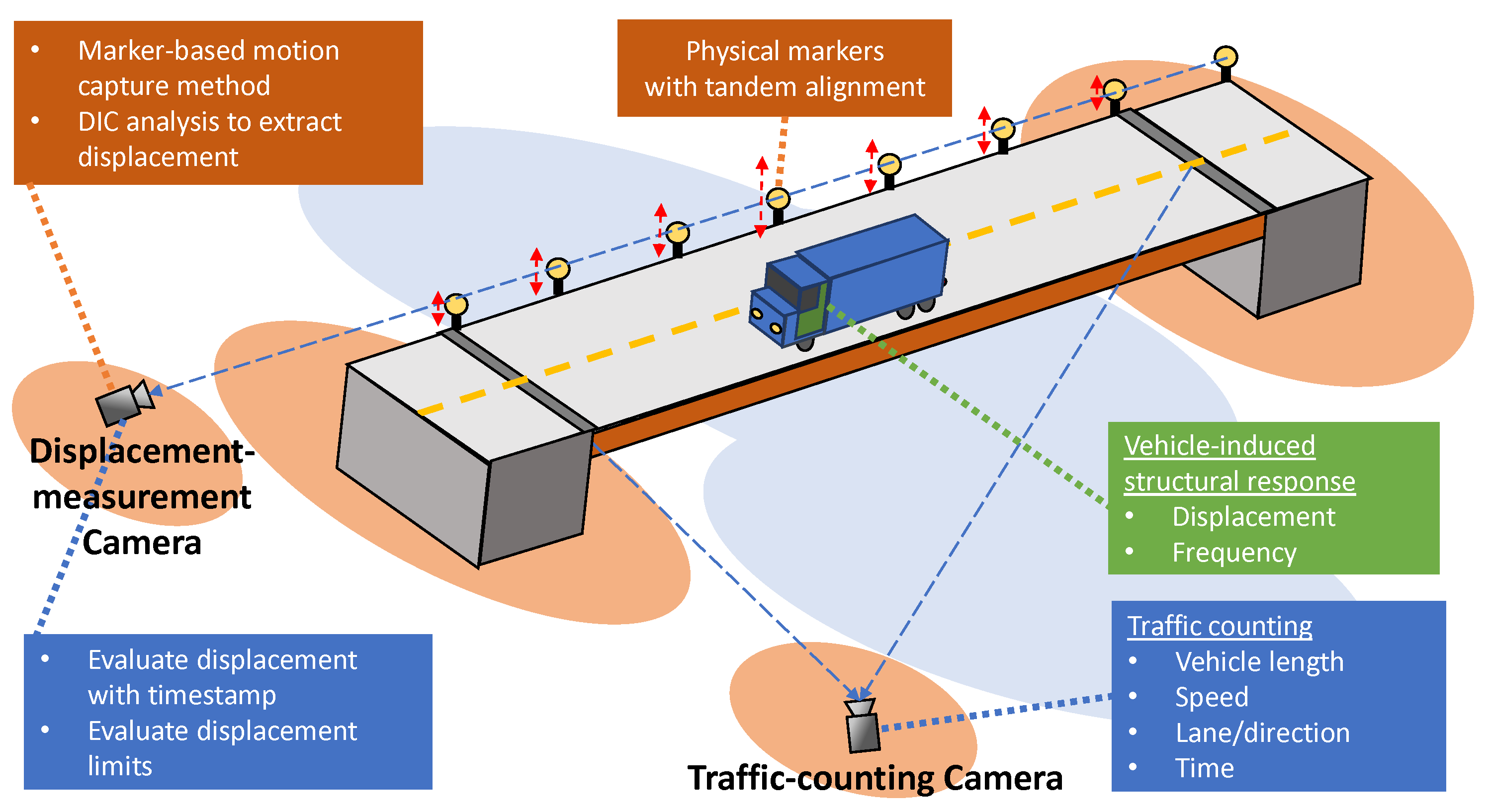
3. Tandem Marker Motion Capture with Side-View Monitoring
3.1. Single-Camera-Based Bridge Displacement Measurement
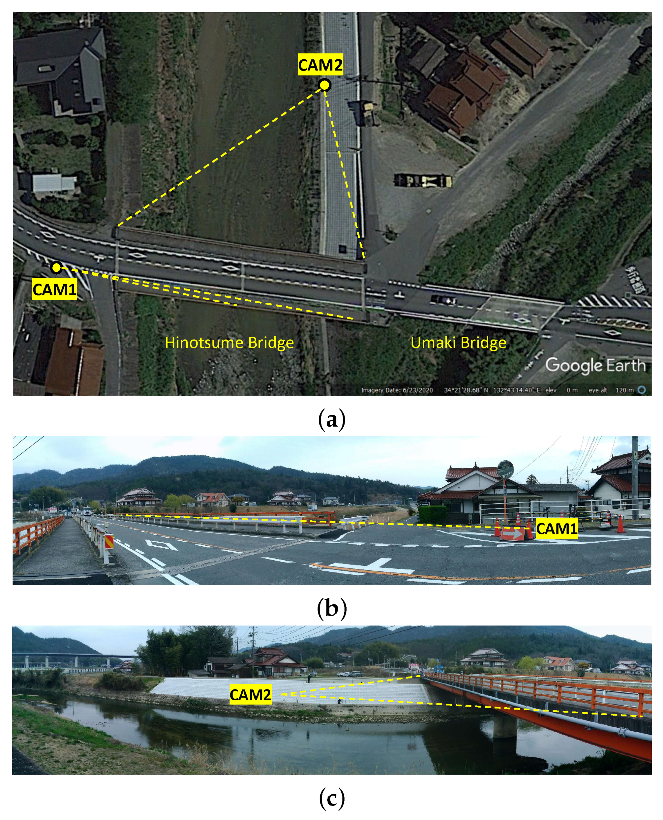
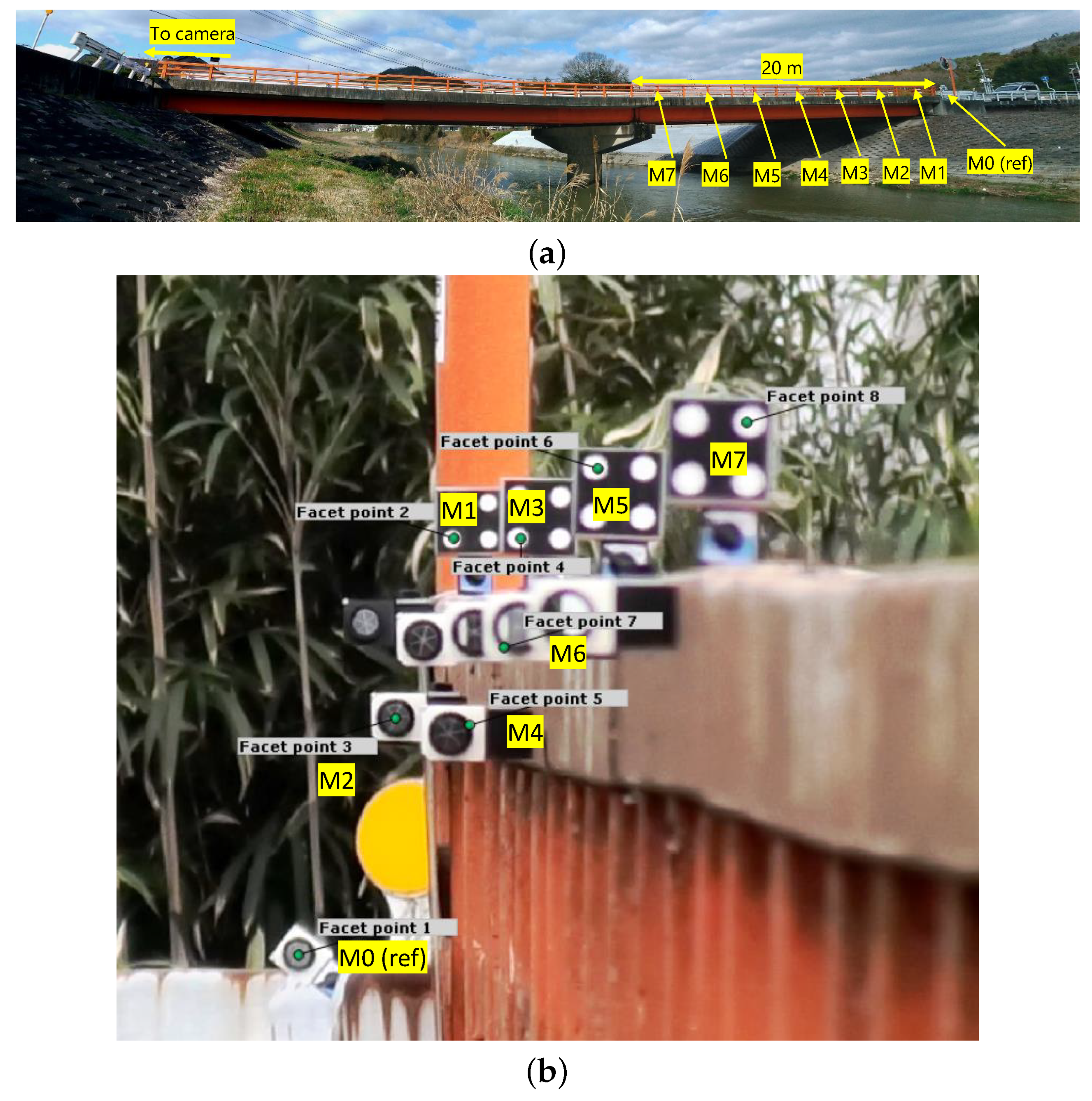
3.2. Field Experiment
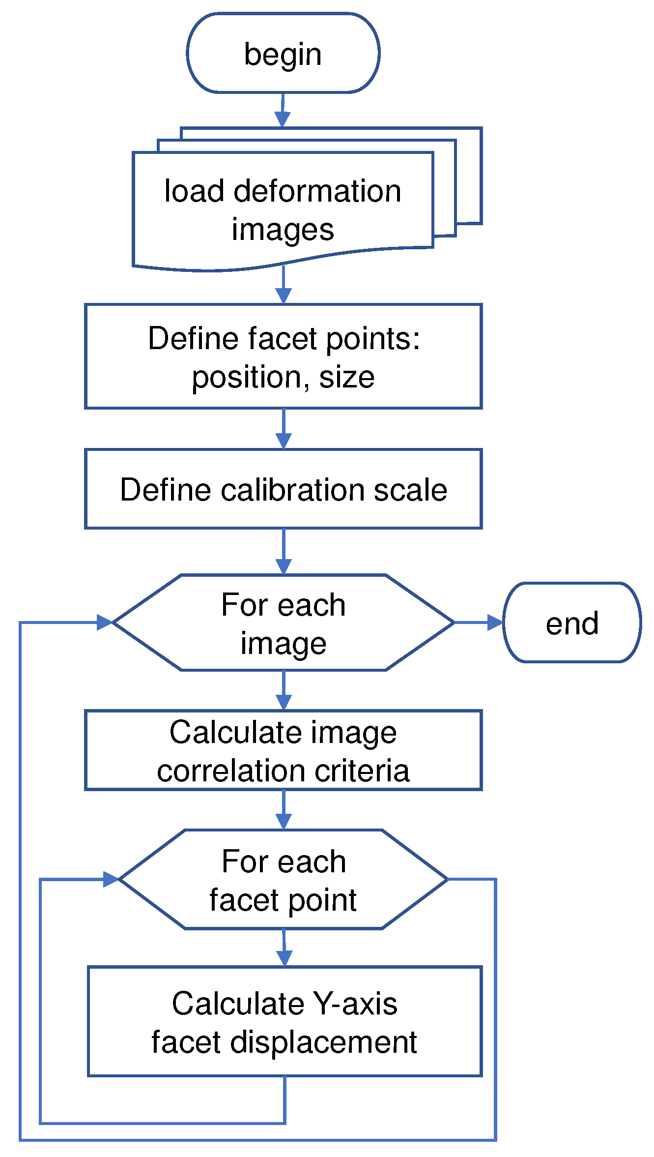
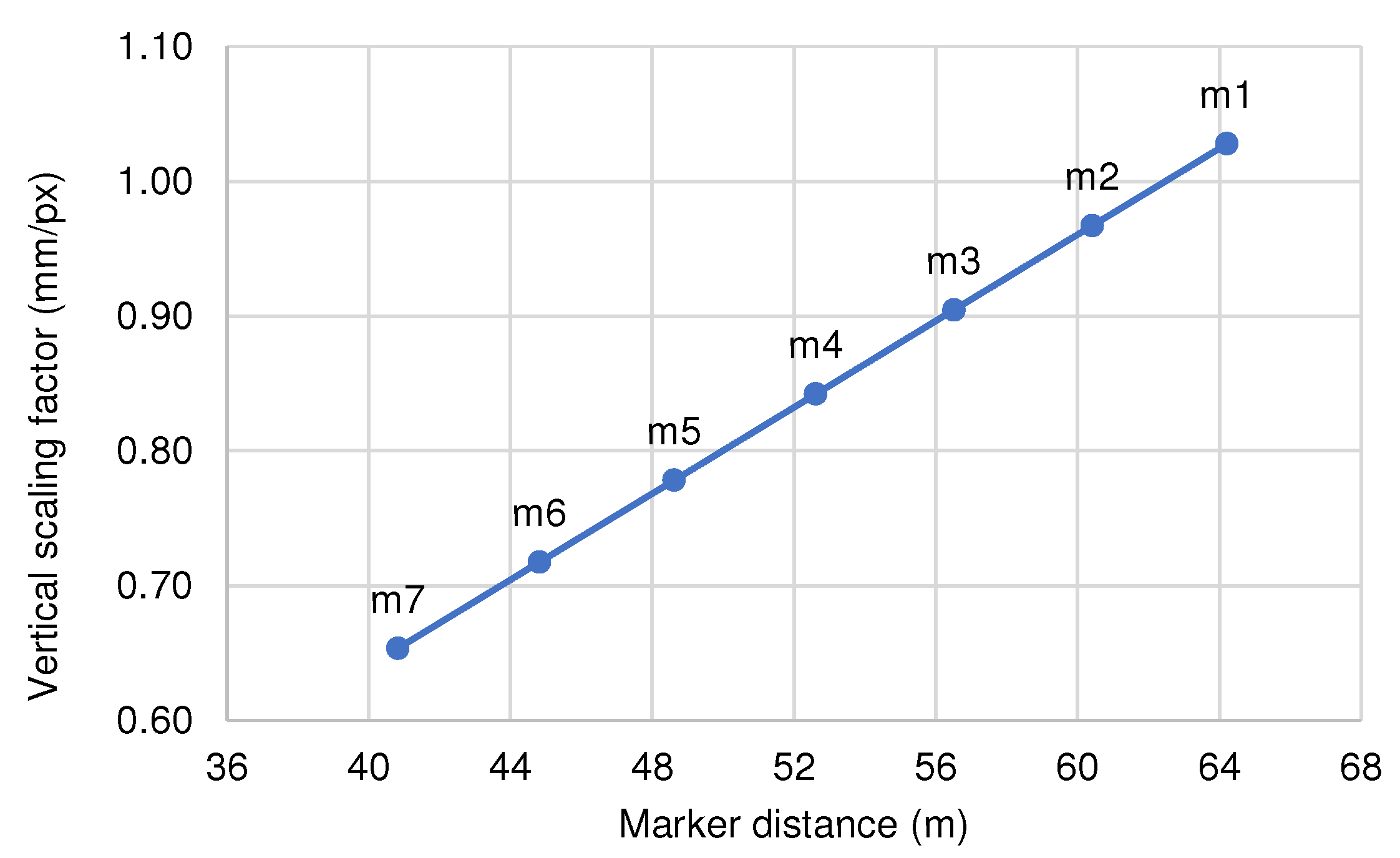
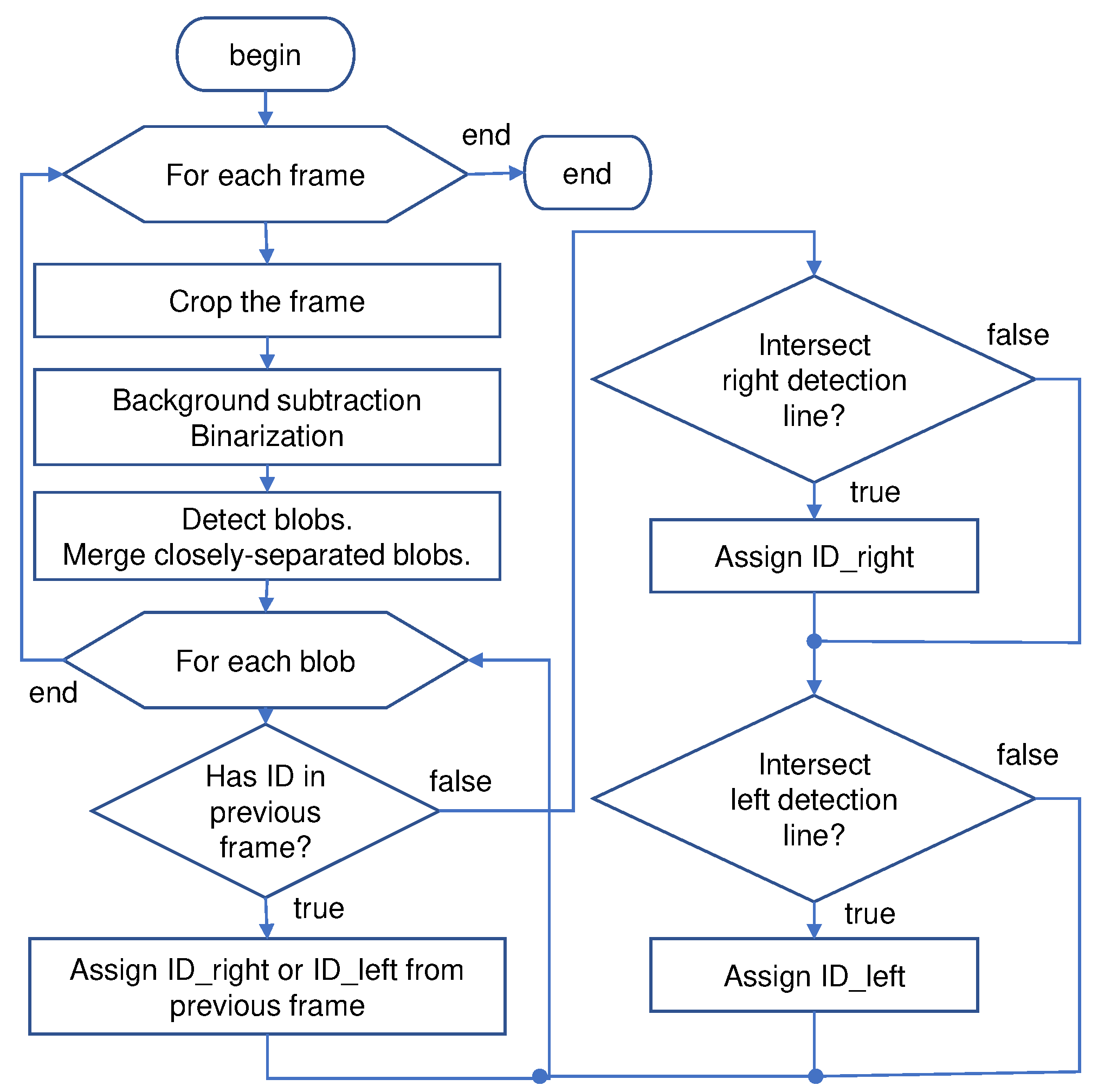
3.3. Implemented Algorithm
3.3.1. Tandem-Marker-Motion Capture from Frontal Camera
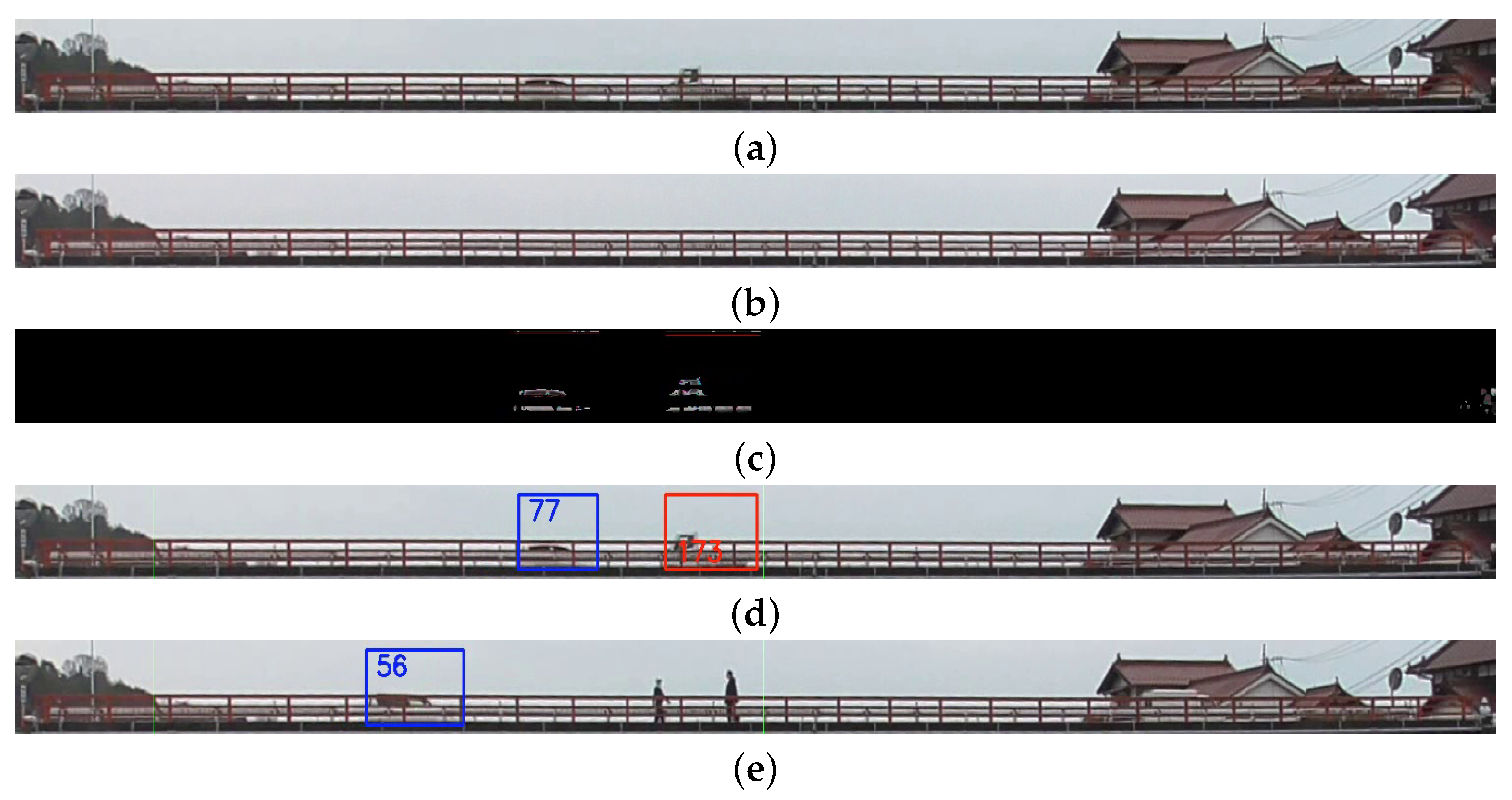
3.3.2. Traffic Counting from Side-View Camera
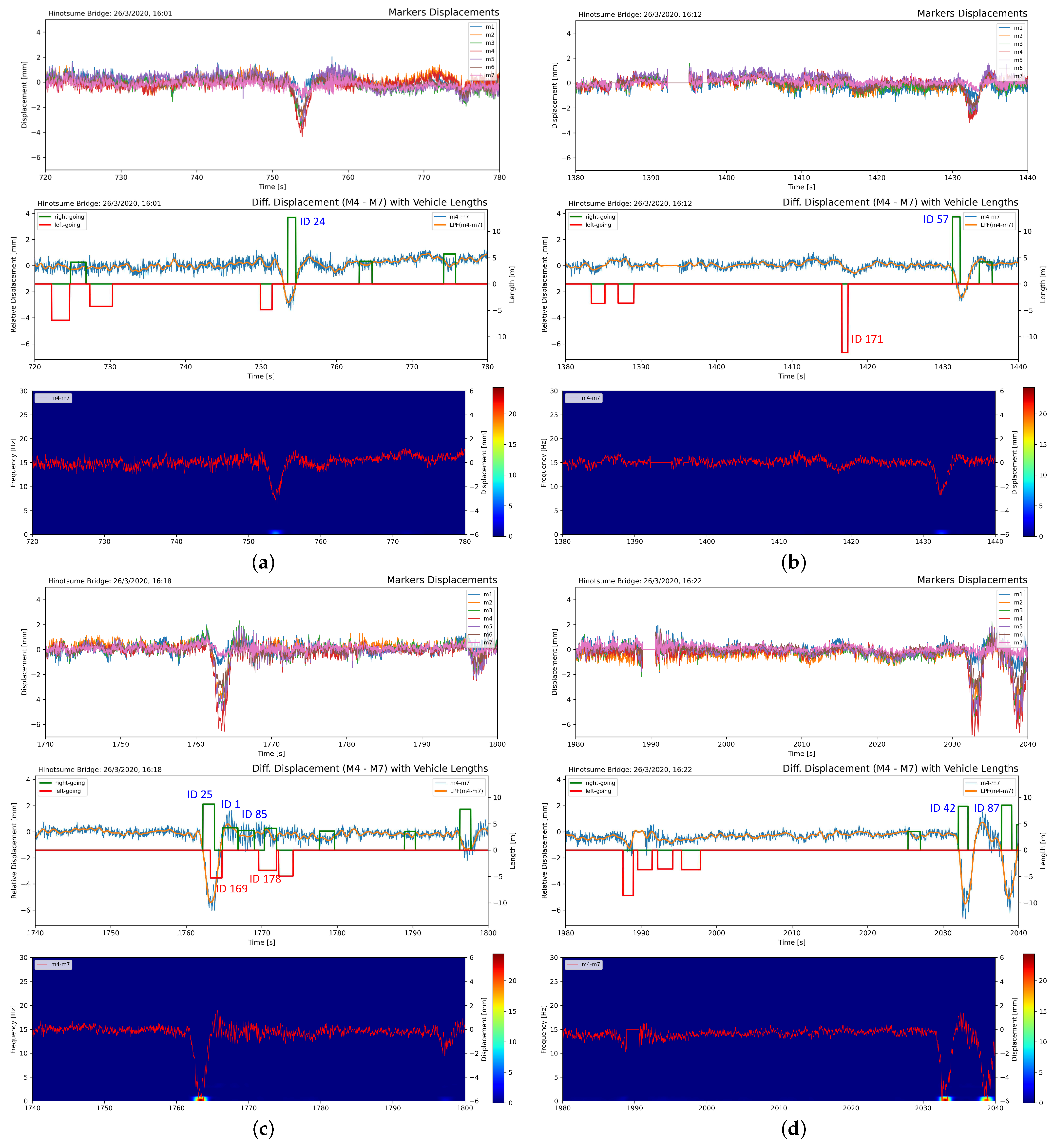
4. Experiment Results and Discussion
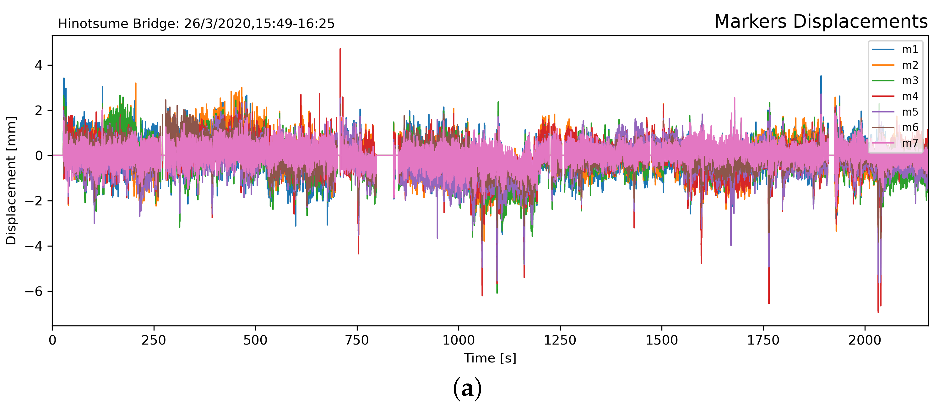
4.1. 35-min Displacement Monitoring
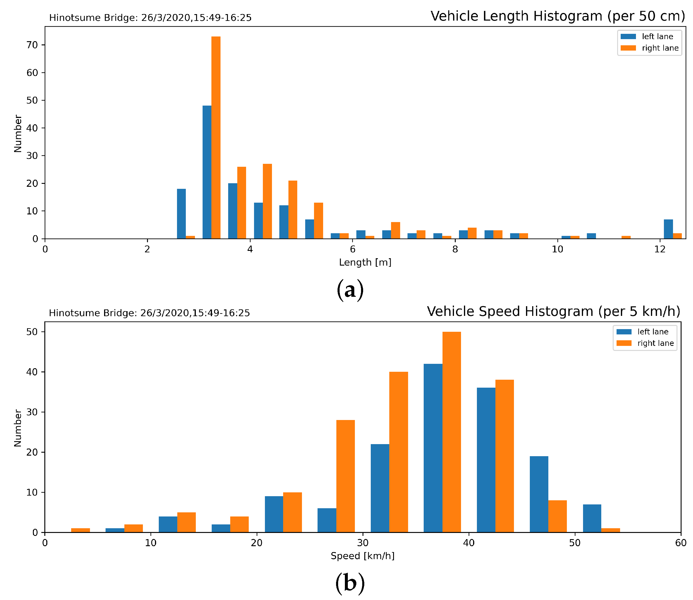
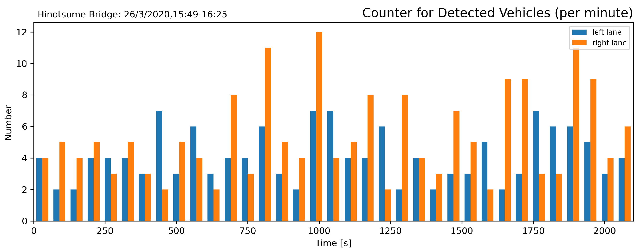
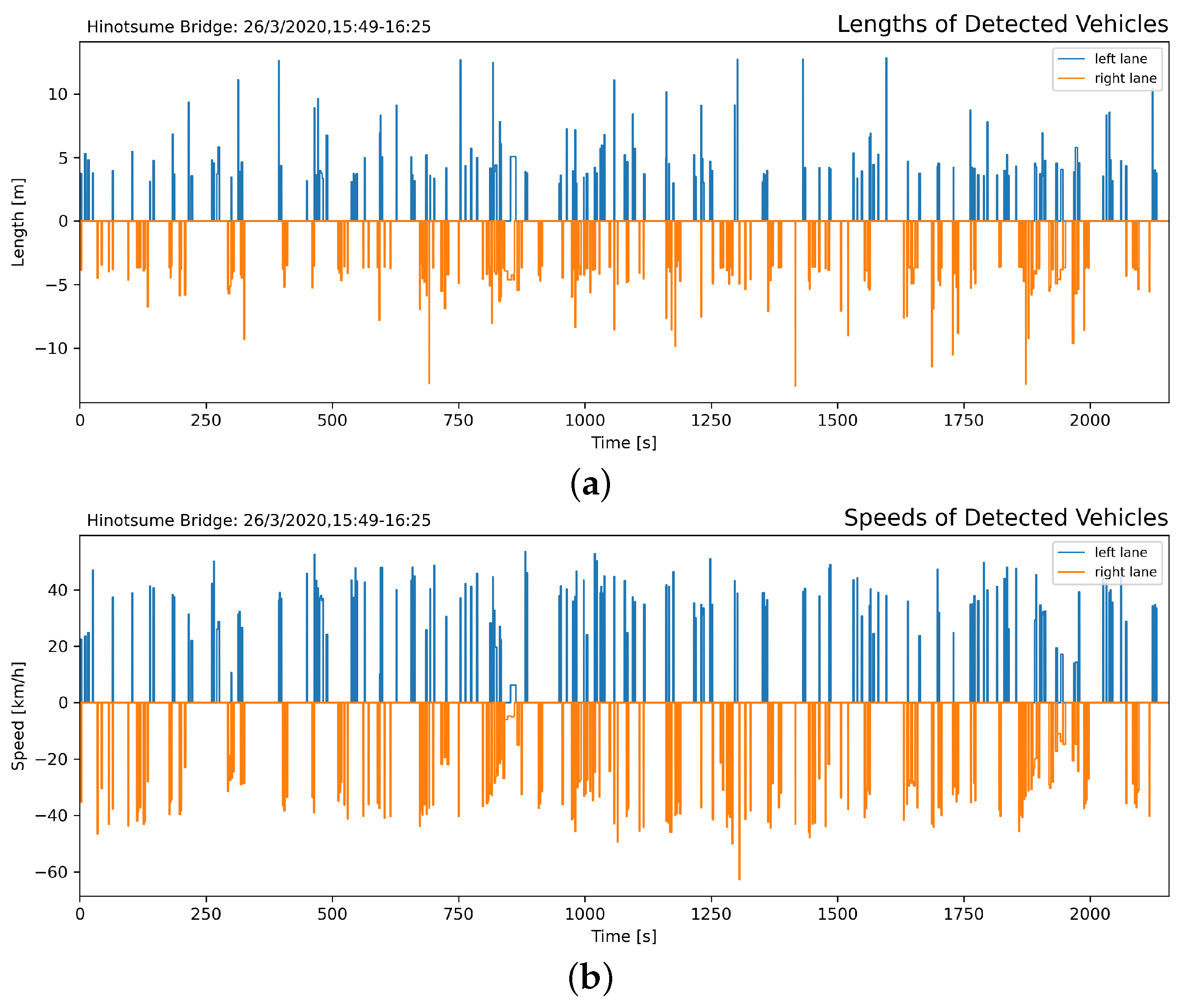
4.2. Traffic Counting
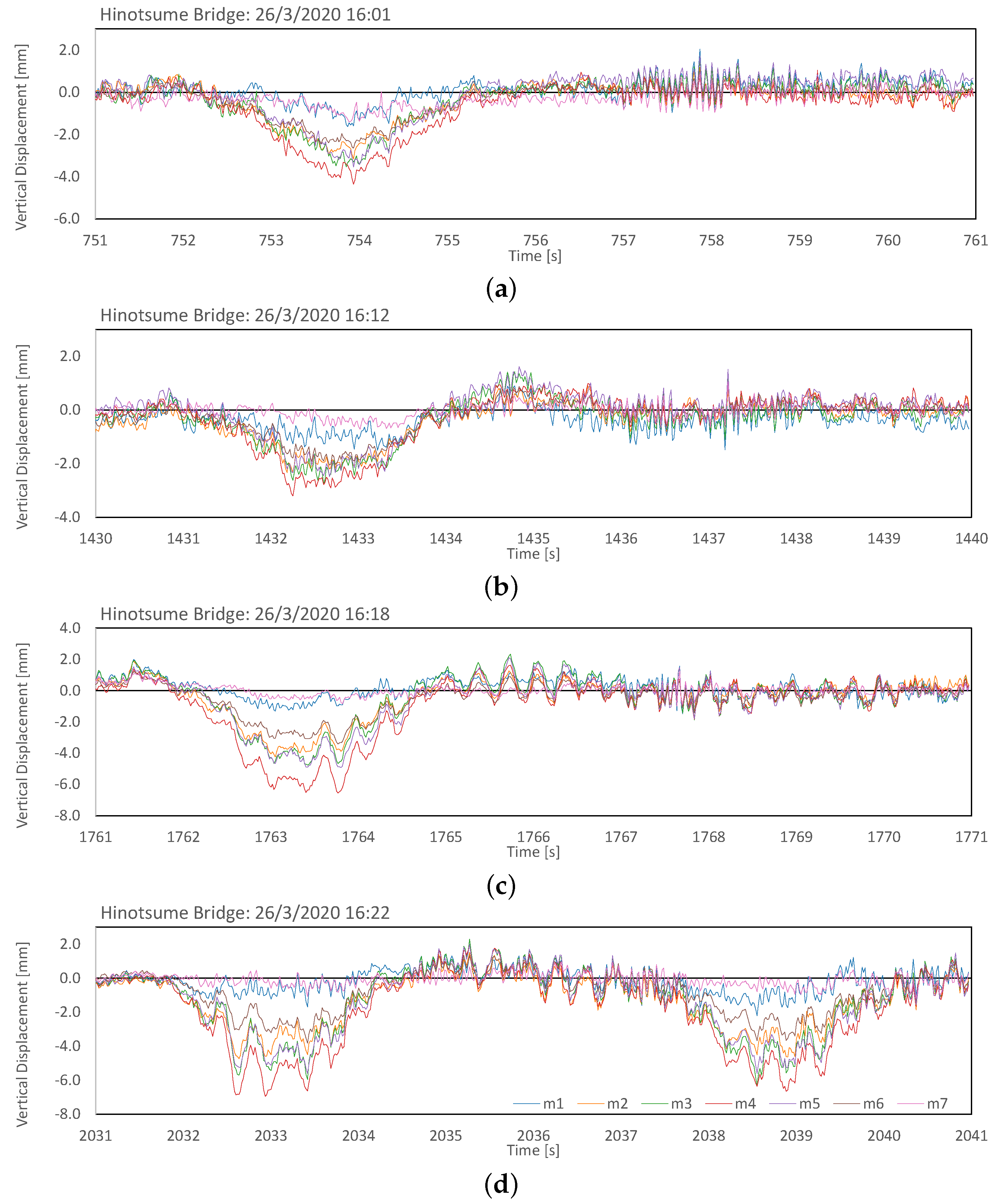
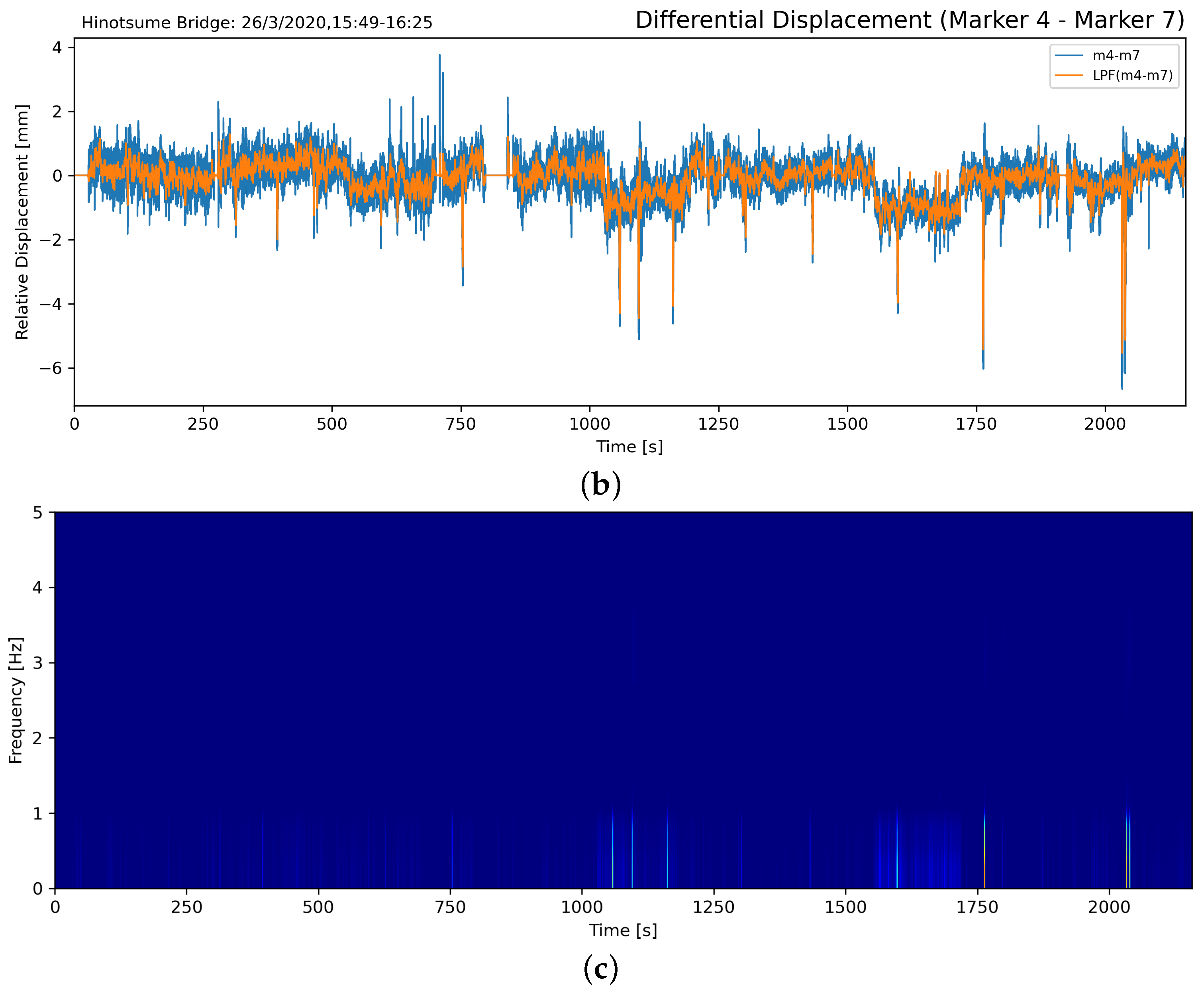
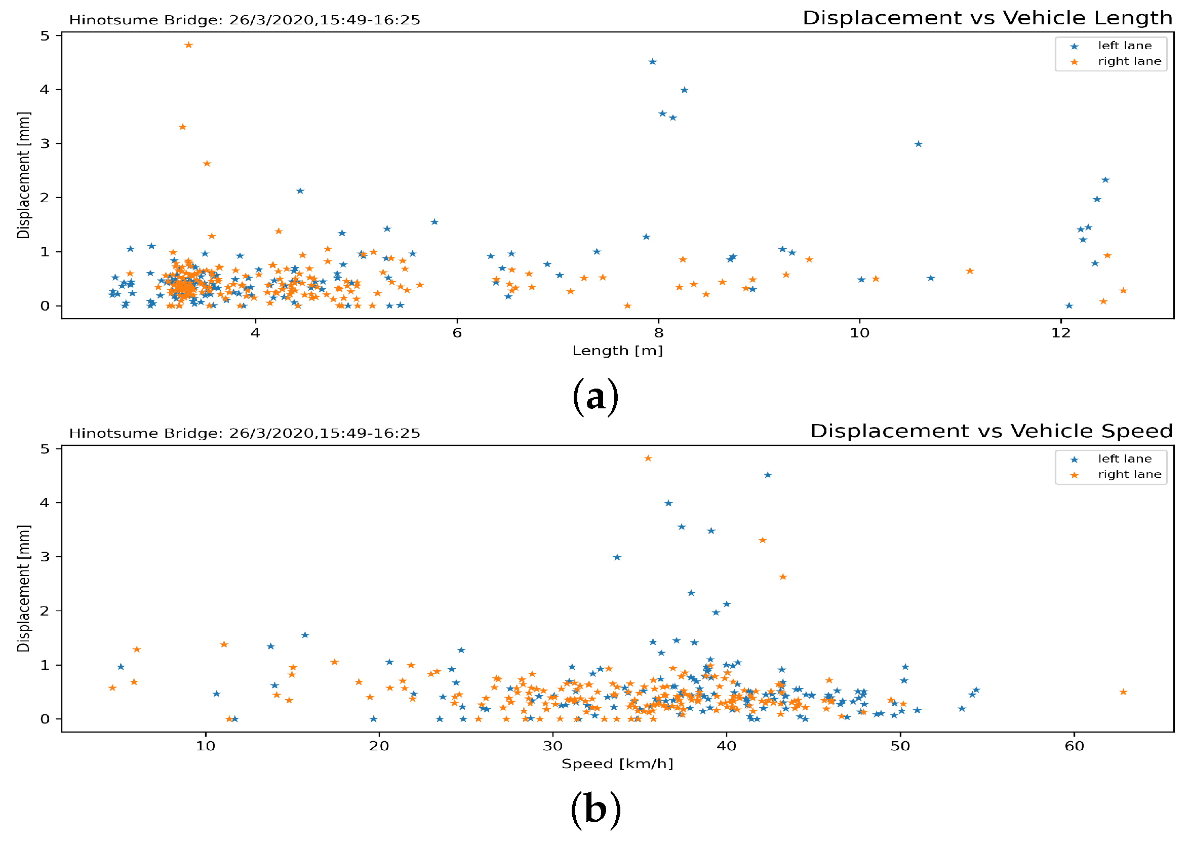
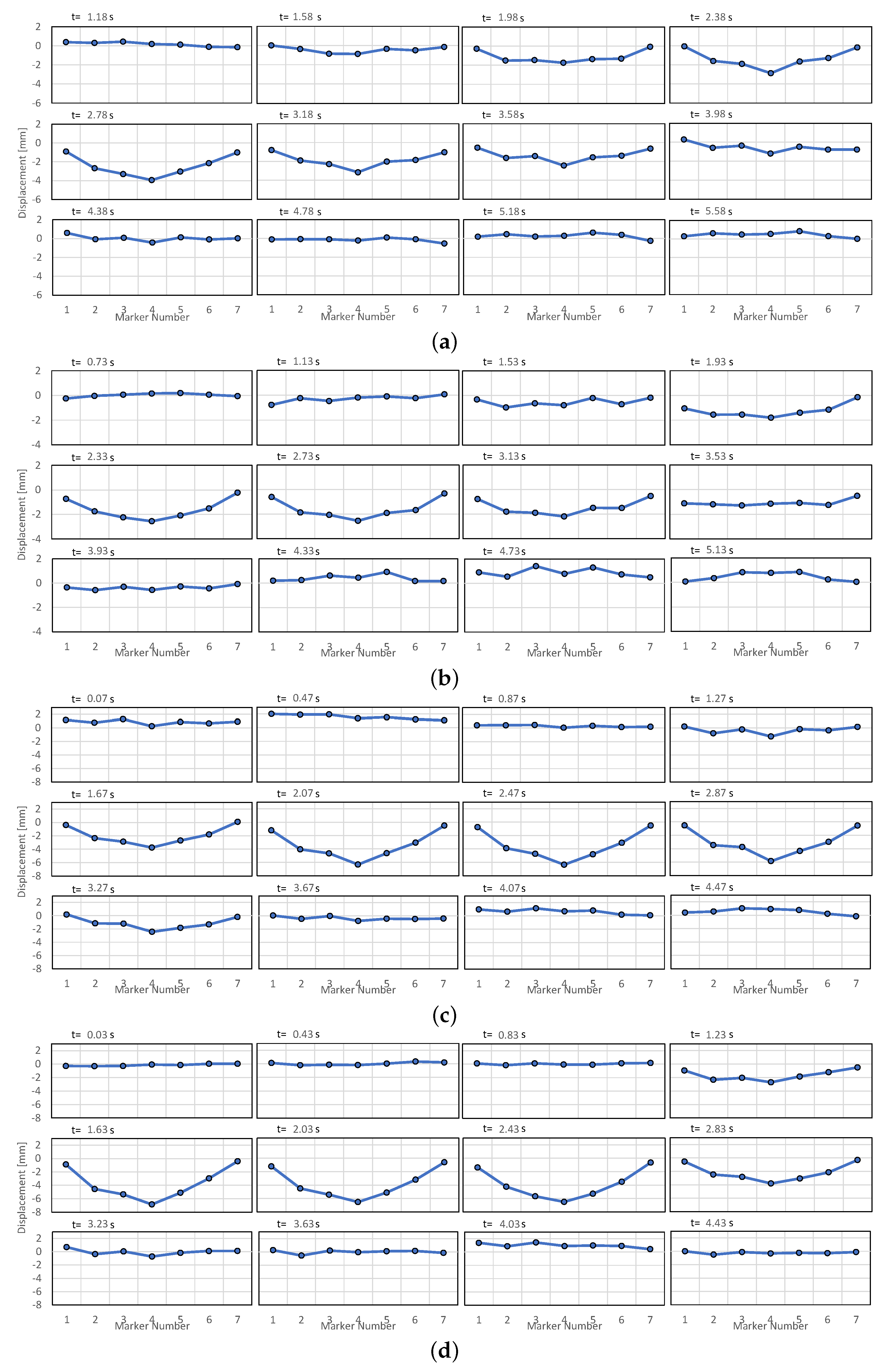
4.3. Structural Response from Large Vehicle Passes
5. Conclusions
Author Contributions
Funding
Data Availability Statement
Acknowledgments
Conflicts of Interest
Appendix A

| Time (ID) | Pass Duration [s] | Traffic Counting Camera |
|---|---|---|
| 16:00 (24) | 1.12 |  |
| 16:06 (20) | 1.82 |  |
| 16:07 (61) | 1.53 |  |
| 16:08 (81) | 1.38 |  |
| 16:15 (13) | 1.58 |  |
| 16:18 (25) | 1.67 |  |
| 16:22 (42) | 1.57 |  |
| 17:23 (87) | 1.62 |  |
References
- Seim, C. Bridge maintenance and safety: A practitioner’s view. In Bridge Maintenance, Safety, Management and Life-Cycle Optimization; Frangopol, D.M., Sause, R., Eds.; CRC Press: Boca Raton, FL, USA, 2010; pp. 3–7. [Google Scholar]
- Bakamwesiga, H.; Mwakali, J.; Thelandersson, S. Nondestructive condition assessment of highway bridges for safety enhancement. In Bridge Maintenance, Safety, Management and Life Extension; CRC Press: Boca Raton, FL, USA, 2014; pp. 1764–1771. [Google Scholar] [CrossRef]
- Farrar, C.R.; Worden, K. An introduction to structural health monitoring. Philos. Trans. R. Soc. A Math. Phys. Eng. Sci. 2007, 365, 303–315. [Google Scholar] [CrossRef] [PubMed]
- Conte, J.P.; He, X.; Moaveni, B.; Masri, S.F.; Caffrey, J.P.; Wahbeh, M.; Tasbihgoo, F.; Whang, D.H.; Elgamal, A. Dynamic Testing of Alfred Zampa Memorial Bridge. J. Struct. Eng. 2008, 134, 1006–1015. [Google Scholar] [CrossRef] [Green Version]
- Fraser, M.; Elgamal, A.; He, X.; Conte, J.P. Sensor Network for Structural Health Monitoring of a Highway Bridge. J. Comput. Civ. Eng. 2010, 24, 11–24. [Google Scholar] [CrossRef] [Green Version]
- Aliansyah, Z.; Shimasaki, K.; Jiang, M.; Takaki, T.; Ishii, I.; Yang, H.; Umemoto, C.; Matsuda, H. A Tandem Marker-Based Motion Capture Method for Dynamic Small Displacement Distribution Analysis. J. Robot. Mechatron. 2019, 31, 671–685. [Google Scholar] [CrossRef]
- AASHTO. AASHTO LRFD Bridge Design Specifications, U.S. Customary Units, 7th ed.; American Association of State Highway and Transportation Officials (AASHTO): Washington, DC, USA, 2014. [Google Scholar]
- Fiore, A.; Marano, G.C. Serviceability Performance Analysis of Concrete Box Girder Bridges Under Traffic-Induced Vibrations by Structural Health Monitoring: A Case Study. Int. J. Civ. Eng. 2018, 16, 553–565. [Google Scholar] [CrossRef]
- Salvermoser, J.; Hadziioannou, C.; Stähler, S.C. Structural monitoring of a highway bridge using passive noise recordings from street traffic. J. Acoust. Soc. Am. 2015, 138, 3864–3872. [Google Scholar] [CrossRef]
- Hester, D.; González, A. A discussion on the merits and limitations of using drive-by monitoring to detect localised damage in a bridge. Mech. Syst. Signal Process. 2017, 90, 234–253. [Google Scholar] [CrossRef] [Green Version]
- Ngeljaratan, L.; Moustafa, M.A. System Identification of Large-Scale Bridges Using Target-Tracking Digital Image Correlation. Front. Built Environ. 2019, 5, 85. [Google Scholar] [CrossRef] [Green Version]
- Dos Santos, R.C.; Larocca, A.P.C.; de Araújo Neto, J.O.; Barbosa, A.C.B.; Oliveira, J.V.M. Detection of a curved bridge deck vibration using robotic total stations for structural health monitoring. J. Civ. Struct. Health Monit. 2019, 9, 63–76. [Google Scholar] [CrossRef]
- Górski, P.; Napieraj, M.; Konopka, E. Variability evaluation of dynamic characteristics of highway steel bridge based on daily traffic-induced vibrations. Measurement 2020, 164, 108074. [Google Scholar] [CrossRef]
- Deng, Y.; Li, A.; Feng, D. Probabilistic Damage Detection of Long-Span Bridges Using Measured Modal Frequencies and Temperature. Int. J. Struct. Stab. Dyn. 2018, 18, 1850126. [Google Scholar] [CrossRef]
- Carden, E.P.; Fanning, P. Vibration Based Condition Monitoring: A Review. Struct. Health Monit. Int. J. 2004, 3, 355–377. [Google Scholar] [CrossRef]
- OBrien, E.; Carey, C.; Keenahan, J. Bridge damage detection using ambient traffic and moving force identification: Bridge Damage Detection and Moving Force Identification. Struct. Control Health Monit. 2015, 22, 1396–1407. [Google Scholar] [CrossRef] [Green Version]
- Gara, F.; Nicoletti, V.; Roia, D.; Dezi, L.; Dall’Asta, A. Dynamic monitoring of an isolated steel arch bridge during static load test. In Proceedings of the 2016 IEEE Workshop on Environmental, Energy, and Structural Monitoring Systems, Bari, Italy, 13–14 June 2016; pp. 1–6. [Google Scholar] [CrossRef]
- Fernstrom, E.V.; Wank, T.R.; Grimmelsman, K.A. Dynamic Testing of a Truss Bridge Using a Vibroseis Truck. In Topics on the Dynamics of Civil Structures; Caicedo, J., Catbas, F., Cunha, A., Racic, V., Reynolds, P., Salyards, K., Eds.; Springer: New York, NY, USA, 2012; Volume 1, pp. 155–163. [Google Scholar] [CrossRef]
- Elhattab, A.; Uddin, N.; OBrien, E. Drive-By Bridge Frequency Identification under Operational Roadway Speeds Employing Frequency Independent Underdamped Pinning Stochastic Resonance (FI-UPSR). Sensors 2018, 18, 4207. [Google Scholar] [CrossRef] [PubMed] [Green Version]
- Malekjafarian, A.; OBrien, E.J. On the use of a passing vehicle for the estimation of bridge mode shapes. J. Sound Vib. 2017, 397, 77–91. [Google Scholar] [CrossRef] [Green Version]
- Ho, H.; Nishio, M. Evaluation of dynamic responses of bridges considering traffic flow and surface roughness. Eng. Struct. 2020, 225, 111256. [Google Scholar] [CrossRef]
- Cantero, D.; McGetrick, P.; Kim, C.W.; OBrien, E. Experimental monitoring of bridge frequency evolution during the passage of vehicles with different suspension properties. Eng. Struct. 2019, 187, 209–219. [Google Scholar] [CrossRef]
- McGetrick, P.J.; González, A.; OBrien, E.J. Theoretical investigation of the use of a moving vehicle to identify bridge dynamic parameters. Insight. Non-Destr. Test Cond. Monit. 2009, 51, 433–438. [Google Scholar] [CrossRef] [Green Version]
- Sadeghi Eshkevari, S.; Matarazzo, T.J.; Pakzad, S.N. Simplified vehicle–bridge interaction for medium to long-span bridges subject to random traffic load. J. Civ. Struct. Health Monit. 2020, 10, 693–707. [Google Scholar] [CrossRef]
- Vaghefi, K.; Oats, R.C.; Harris, D.K.; Ahlborn, T.T.M.; Brooks, C.N.; Endsley, K.A.; Roussi, C.; Shuchman, R.; Burns, J.W.; Dobson, R. Evaluation of Commercially Available Remote Sensors for Highway Bridge Condition Assessment. J. Bridge Eng. 2012, 17, 886–895. [Google Scholar] [CrossRef]
- Khoo, S.W.; Karuppanan, S.; Tan, C.S. A Review of Surface Deformation and Strain Measurement Using Two-Dimensional Digital Image Correlation. Metrol. Meas. Syst. 2016, 23, 461–480. [Google Scholar] [CrossRef]
- Tong, W. Formulation of Lucas-Kanade Digital Image Correlation Algorithms for Non-contact Deformation Measurements: A Review: Lucas-Kanade Digital Image Correlation Algorithms. Strain 2013, 49, 313–334. [Google Scholar] [CrossRef]
- Pan, B.; Yu, L.; Zhang, Q. Review of single-camera stereo-digital image correlation techniques for full-field 3D shape and deformation measurement. Sci. China Technol. Sci. 2018, 61, 2–20. [Google Scholar] [CrossRef] [Green Version]
- Pan, B. Digital image correlation for surface deformation measurement: Historical developments, recent advances and future goals. Meas. Sci. Technol. 2018, 29, 082001. [Google Scholar] [CrossRef]
- Diamond, D.; Heyns, P.; Oberholster, A. Accuracy evaluation of sub-pixel structural vibration measurements through optical flow analysis of a video sequence. Measurement 2017, 95, 166–172. [Google Scholar] [CrossRef]
- Gencturk, B.; Hossain, K.; Kapadia, A.; Labib, E.; Mo, Y.L. Use of digital image correlation technique in full-scale testing of prestressed concrete structures. Measurement 2014, 47, 505–515. [Google Scholar] [CrossRef]
- Hamrat, M.; Boulekbache, B.; Chemrouk, M.; Amziane, S. Flexural cracking behavior of normal strength, high strength and high strength fiber concrete beams, using Digital Image Correlation technique. Constr. Build. Mater. 2016, 106, 678–692. [Google Scholar] [CrossRef]
- Beberniss, T.J.; Ehrhardt, D.A. High-speed 3D digital image correlation vibration measurement: Recent advancements and noted limitations. Mech. Syst. Signal Process. 2017, 86, 35–48. [Google Scholar] [CrossRef]
- Pan, B.; Qian, K.; Xie, H.; Asundi, A. Two-dimensional digital image correlation for in-plane displacement and strain measurement: A review. Meas. Sci. Technol. 2009, 20, 062001. [Google Scholar] [CrossRef]
- Ahlborn, T.M.; Harris, D.K.; Vaghefi, K.; Oats, R.C. An Evaluation of Commercially Available Remote Sensors for Assessing Highway Bridge Condition; Technical Report; Michigan Technological University: Ann Arbor, MI, USA, 2010. [Google Scholar]
- Feng, D.; Feng, M.Q. Experimental validation of cost-effective vision-based structural health monitoring. Mech. Syst. Signal Process. 2017, 88, 199–211. [Google Scholar] [CrossRef]
- Luo, L.; Feng, M.Q.; Wu, Z.Y. Robust vision sensor for multi-point displacement monitoring of bridges in the field. Eng. Struct. 2018, 163, 255–266. [Google Scholar] [CrossRef]
- Luo, L.; Feng, M.Q.; Wu, J. A comprehensive alleviation technique for optical-turbulence-induced errors in vision-based displacement measurement. Struct. Control Health Monit. 2020, 27. [Google Scholar] [CrossRef]
- Kohm, M.; Stempniewski, L. Beam tests for a wireless modal-based bridge monitoring system. In Proceedings of the 20th Congress of IABSE 2019: The Evolving Metropolis, New York, NY, USA, 4–6 September 2019; pp. 669–682. [Google Scholar]
- Tang, Z.; Shimasaki, K.; Jiang, M.; Takaki, T.; Ishii, I.; Koga, A.; Matsuda, H. Ironworks Conveyor Monitoring Using Mirror-drive High-speed Active Vision. ISIJ Int. 2020, 60, 960–970. [Google Scholar] [CrossRef]
- Bellucci, P.; Cipriani, E. Data accuracy on automatic traffic counting: The SMART project results. Eur. Transp. Res. Rev. 2010, 2, 175–187. [Google Scholar] [CrossRef] [Green Version]
- Arinaldi, A.; Pradana, J.A.; Gurusinga, A.A. Detection and classification of vehicles for traffic video analytics. Procedia Comput. Sci. 2018, 144, 259–268. [Google Scholar] [CrossRef]
- Ince, E. Measuring traffic flow and classifying vehicle types: A surveillance video based approach. Turk. J. Electr. Eng. Comput. Sci. 2011, 19, 607–620. [Google Scholar]
- Rabbouch, H.; Saâdaoui, F.; Mraihi, R. Unsupervised video summarization using cluster analysis for automatic vehicles counting and recognizing. Neurocomputing 2017, 260, 157–173. [Google Scholar] [CrossRef]
- Liu, F.; Zeng, Z.; Jiang, R. A video-based real-time adaptive vehicle-counting system for urban roads. PLoS ONE 2017, 12, e0186098. [Google Scholar] [CrossRef] [Green Version]
- Bharadwaj, N.; Kumar, P.; Arkatkar, S.; Maurya, A.; Joshi, G. Traffic data analysis using image processing technique on Delhi–Gurgaon expressway. Curr. Sci. 2016, 110, 16. [Google Scholar]
- Fu, H.; Ma, H.; Liu, Y.; Lu, D. A vehicle classification system based on hierarchical multi-SVMs in crowded traffic scenes. Neurocomputing 2016, 211, 182–190. [Google Scholar] [CrossRef]
- Kawakatsu, T.; Kakitani, A.; Aihara, K.; Takasu, A.; Adachi, J. Traffic Surveillance System for Bridge Vibration Analysis. In Proceedings of the 2017 IEEE International Conference on Information Reuse and Integration, San Diego, CA, USA, 4–6 August 2017; pp. 69–74. [Google Scholar] [CrossRef]
- Lin, J.P.; Sun, M.T. A YOLO-Based Traffic Counting System. In Proceedings of the 2018 Conference on Technologies and Applications of Artificial Intelligence, Taichung, Taiwan, 30 November–2 December 2018; pp. 82–85. [Google Scholar] [CrossRef]
- Sun, M.; Wang, Y.; Li, T.; Lv, J.; Wu, J. Vehicle counting in crowded scenes with multi-channel and multi-task convolutional neural networks. J. Vis. Commun. Image Represent. 2017, 49, 412–419. [Google Scholar] [CrossRef]
- Khan, S.M.; Atamturktur, S.; Chowdhury, M.; Rahman, M. Integration of Structural Health Monitoring and Intelligent Transportation Systems for Bridge Condition Assessment: Current Status and Future Direction. IEEE Trans. Intell. Transp. Syst. 2016, 17, 2107–2122. [Google Scholar] [CrossRef]
- Dong, C.Z.; Bas, S.; Catbas, F.N. A portable monitoring approach using cameras and computer vision for bridge load rating in smart cities. J. Civ. Struct. Health Monit. 2020, 10, 1001–1021. [Google Scholar] [CrossRef]
- Chen, C.C.; Wu, W.H.; Tseng, H.Z.; Chen, C.H.; Lai, G. Application of digital photogrammetry techniques in identifying the mode shape ratios of stay cables with multiple camcorders. Measurement 2015, 75, 134–146. [Google Scholar] [CrossRef]
- Catbas, F.N.; Zaurin, R.; Gul, M.; Gokce, H.B. Sensor Networks, Computer Imaging, and Unit Influence Lines for Structural Health Monitoring: Case Study for Bridge Load Rating. J. Bridge Eng. 2012, 17, 662–670. [Google Scholar] [CrossRef]
- Zaurin, R.; Khuc, T.; Catbas, F.N. Hybrid Sensor-Camera Monitoring for Damage Detection: Case Study of a Real Bridge. J. Bridge Eng. 2016, 21, 05016002. [Google Scholar] [CrossRef]
- Ge, L.; Dan, D.; Li, H. An accurate and robust monitoring method of full-bridge traffic load distribution based on YOLO-v3 machine vision. Struct. Control Health Monit. 2020, 27. [Google Scholar] [CrossRef]
- Hu, P.F.; Tian, Z.Z.; Liu, H.C. Traffic Counting Errors Due to Occlusion in Video Image Vehicle Detection Systems. In ICCTP 2010; American Society of Civil Engineers: Beijing, China, 2010; pp. 2408–2419. [Google Scholar] [CrossRef]
- Sánchez, A.; Suárez, P.D.; Conci, A.; Nunes, E.O. Video-Based Distance Traffic Analysis: Application to Vehicle Tracking and Counting. Comput. Sci. Eng. 2011, 13. [Google Scholar] [CrossRef]
- Miao, S.; Knobbe, A.; Koenders, E.; Bosma, C. Analysis of Traffic Effects on a Dutch Highway Bridge. IABSE Symp. Rep. 2013, 99, 357–364. [Google Scholar] [CrossRef] [Green Version]
- Jian, X.; Xia, Y.; Lozano-Galant, J.A.; Sun, L. Traffic Sensing Methodology Combining Influence Line Theory and Computer Vision Techniques for Girder Bridges. J. Sens. 2019, 2019, 3409525. [Google Scholar] [CrossRef] [Green Version]
- Grubb, M.A.; Wilson, K.E.; White, C.D.; Nickas, W.N. Load and Resistance Factor Design (LRFD) for Highway Bridge Superstructures Reference Manual; Technical Report FHWA-NHI-15-047; Federal Highway Administration: Arlington, VA, USA, 2015.
- FHWA Office of Policy. Comprehensive Truck Size and Weight Study; Technical Report FHWA-PL-00-029; U.S. Department of Transportation: Washington, DC, USA, 2000; Volume 3, Chapter 6.
- Feng, D.; Feng, M.Q. Output-only damage detection using vehicle-induced displacement response and mode shape curvature index: Damage Detection Using Vehicle-Induced Displacement and MSC Index. Struct. Control Health Monit. 2016, 23, 1088–1107. [Google Scholar] [CrossRef]


| Bridge Construction | Load Type | Displacement Limit |
|---|---|---|
| steel, aluminum, or concrete | vehicular only | span/800 |
| steel, aluminum, or concrete | compound | span/1000 |
| steel, aluminum, or concrete (cantilever) | vehicular only | span/300 |
| steel, aluminum, or concrete (cantilever) | compound | span/325 |
| timber | compound | span/425 |
| Configuration | Gross Weight (ton) | Outside Axle Spread (m) |
|---|---|---|
| Two-axle truck | 13.64 | 7.85 |
| Three-axle truck * | 24.55 | 10.67 |
| Four-axle trailer | 29.09 | 11.13 |
| Five-axle trailer | 36.36 | 20.21 |
| Six-axle trailer | 40.91 | 20.37 |
| Five-axle double trailer | 36.36 | 23.26 |
| Seven-axle double trailer ** | 54.55 | 32.41 |
| Eight-axle double trailer ** | 56.36 | 27.84 |
| Nine-axle double trailer ** | 67.27 | 40.03 |
| Seven-axle triple trailer ** | 60.00 | 33.29 |
| Time (Vehicle ID) | Vehicle | Length (m) | Speed (km/h) |
|---|---|---|---|
| 16:01 (24) |  | 12.27 | 37.11 |
| 16:12 (171 and 57) | 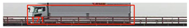  | 12.62 12.36 | 43.09 39.38 |
| 16:18 (25) |  | 8.26 | 36.65 |
| 16:22 (42 and 87) |  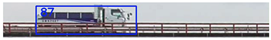 | 7.94 8.14 | 42.36 39.11 |
Publisher’s Note: MDPI stays neutral with regard to jurisdictional claims in published maps and institutional affiliations. |
© 2021 by the authors. Licensee MDPI, Basel, Switzerland. This article is an open access article distributed under the terms and conditions of the Creative Commons Attribution (CC BY) license (https://creativecommons.org/licenses/by/4.0/).
Share and Cite
Aliansyah, Z.; Shimasaki, K.; Senoo, T.; Ishii, I.; Umemoto, S. Single-Camera-Based Bridge Structural Displacement Measurement with Traffic Counting. Sensors 2021, 21, 4517. https://doi.org/10.3390/s21134517
Aliansyah Z, Shimasaki K, Senoo T, Ishii I, Umemoto S. Single-Camera-Based Bridge Structural Displacement Measurement with Traffic Counting. Sensors. 2021; 21(13):4517. https://doi.org/10.3390/s21134517
Chicago/Turabian StyleAliansyah, Zulhaj, Kohei Shimasaki, Taku Senoo, Idaku Ishii, and Shuji Umemoto. 2021. "Single-Camera-Based Bridge Structural Displacement Measurement with Traffic Counting" Sensors 21, no. 13: 4517. https://doi.org/10.3390/s21134517
APA StyleAliansyah, Z., Shimasaki, K., Senoo, T., Ishii, I., & Umemoto, S. (2021). Single-Camera-Based Bridge Structural Displacement Measurement with Traffic Counting. Sensors, 21(13), 4517. https://doi.org/10.3390/s21134517