
Comparison of Direct Intersection and Sonogram Methods for Acoustic Indoor Localization of Persons

 ,
,  , , , , , , , and
Abstract
:1. Introduction
2. Related Work
2.1. RF-RSSI
2.2. RF-Radar
2.3. Ultrasonic Presence Detection and Localization
2.4. Ultrasonic Indoor Mapping
2.5. Algorithms
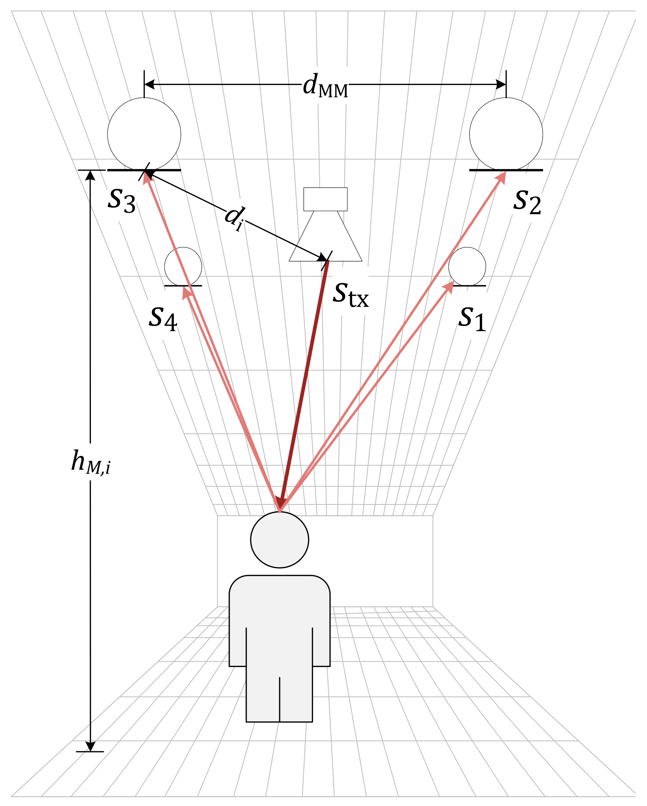
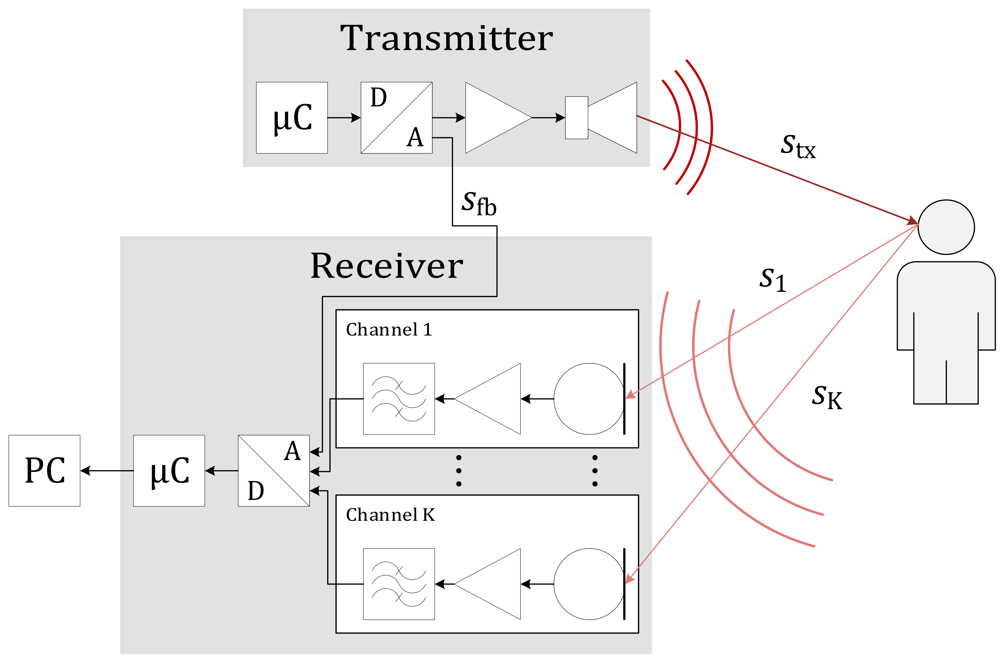
3. System Overview
3.1. Signal Waveform
3.2. Hardware Overview
3.3. Data Acquisition
3.3.1. Channel Phase Synchronization
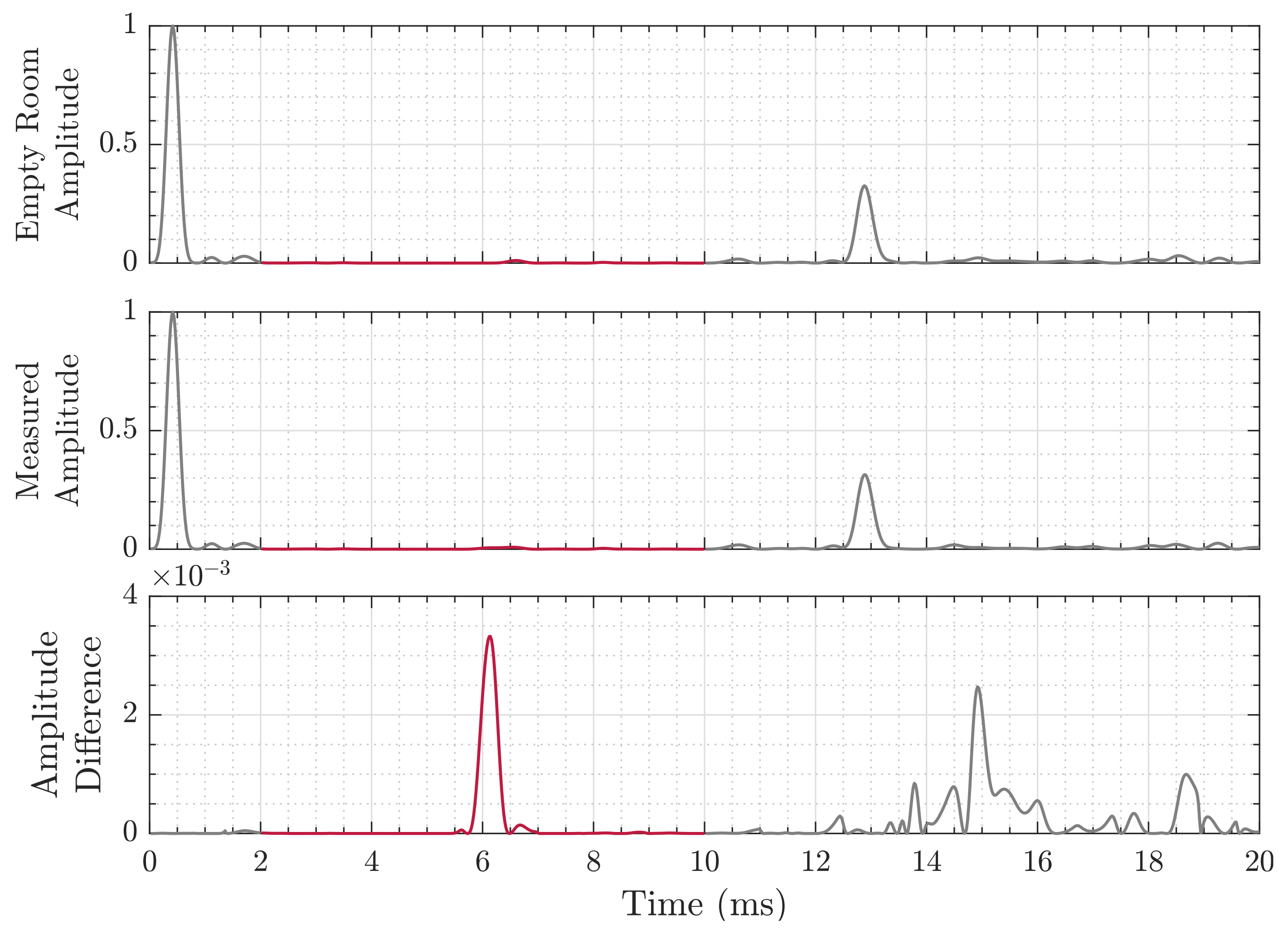
3.3.2. Baseline Removal
3.3.3. Time-Gating
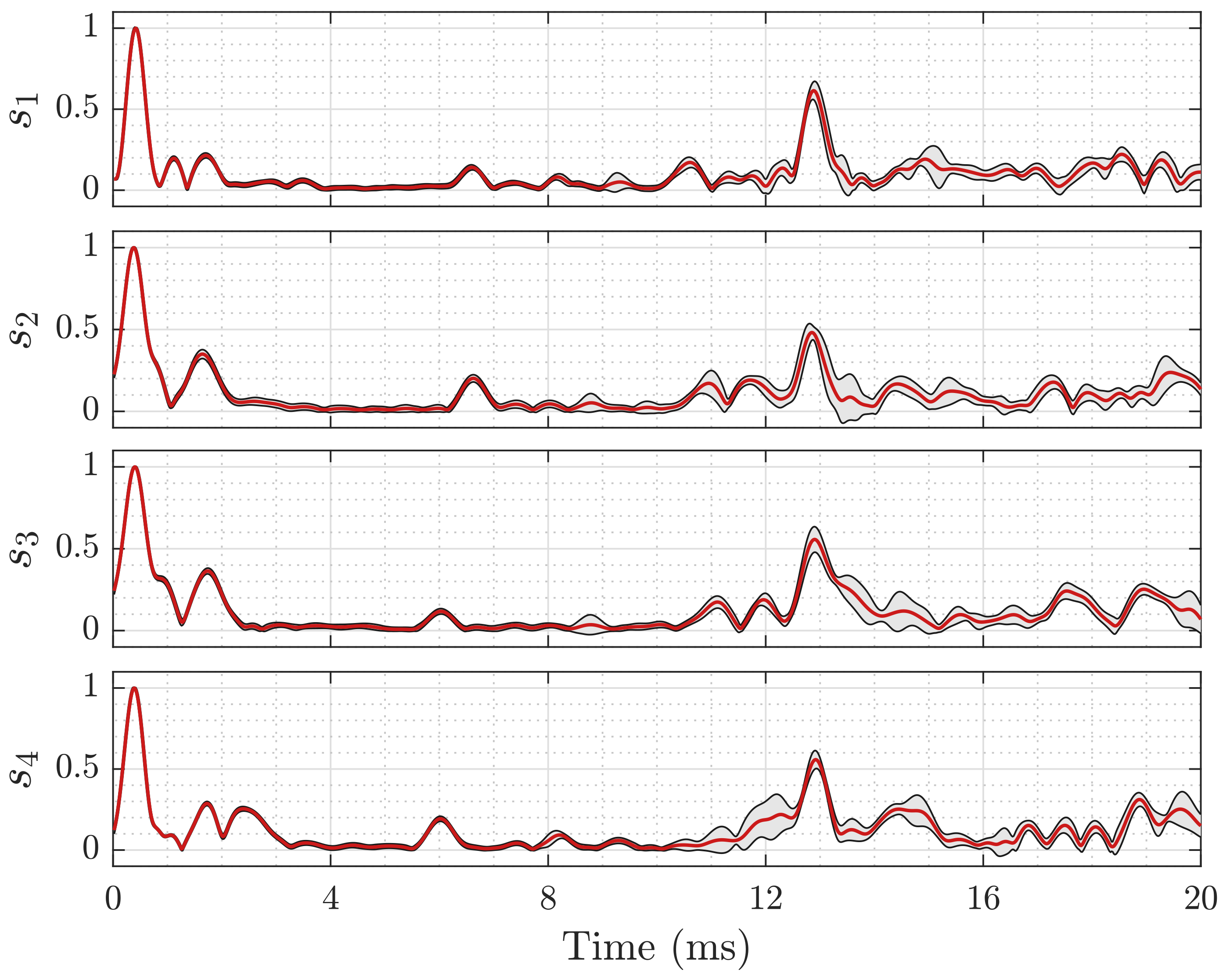
3.3.4. Echo Profile
3.3.5. Distance Maps
3.4. Data Processing
3.4.1. Direct Intersection
| Algorithm 1: Direct Intersection Estimation [56,57]. |
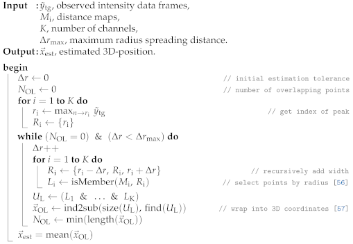 |
3.4.2. Sonogram
| Algorithm 2: Sonogram Estimation [58,59]. |
 |
4. Experiments
4.1. Set-Up
4.2. Results
4.2.1. Room Properties and Impulse Response
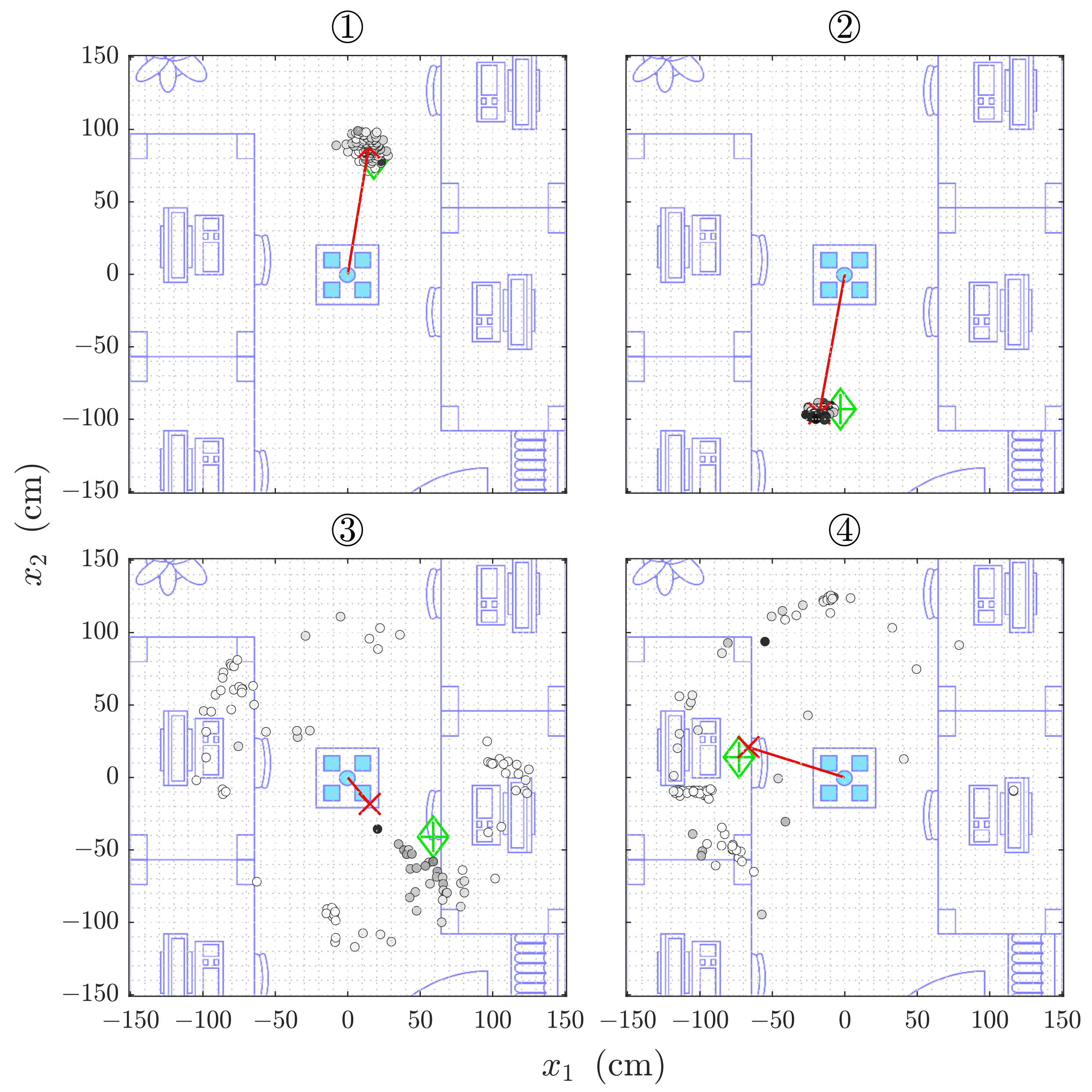
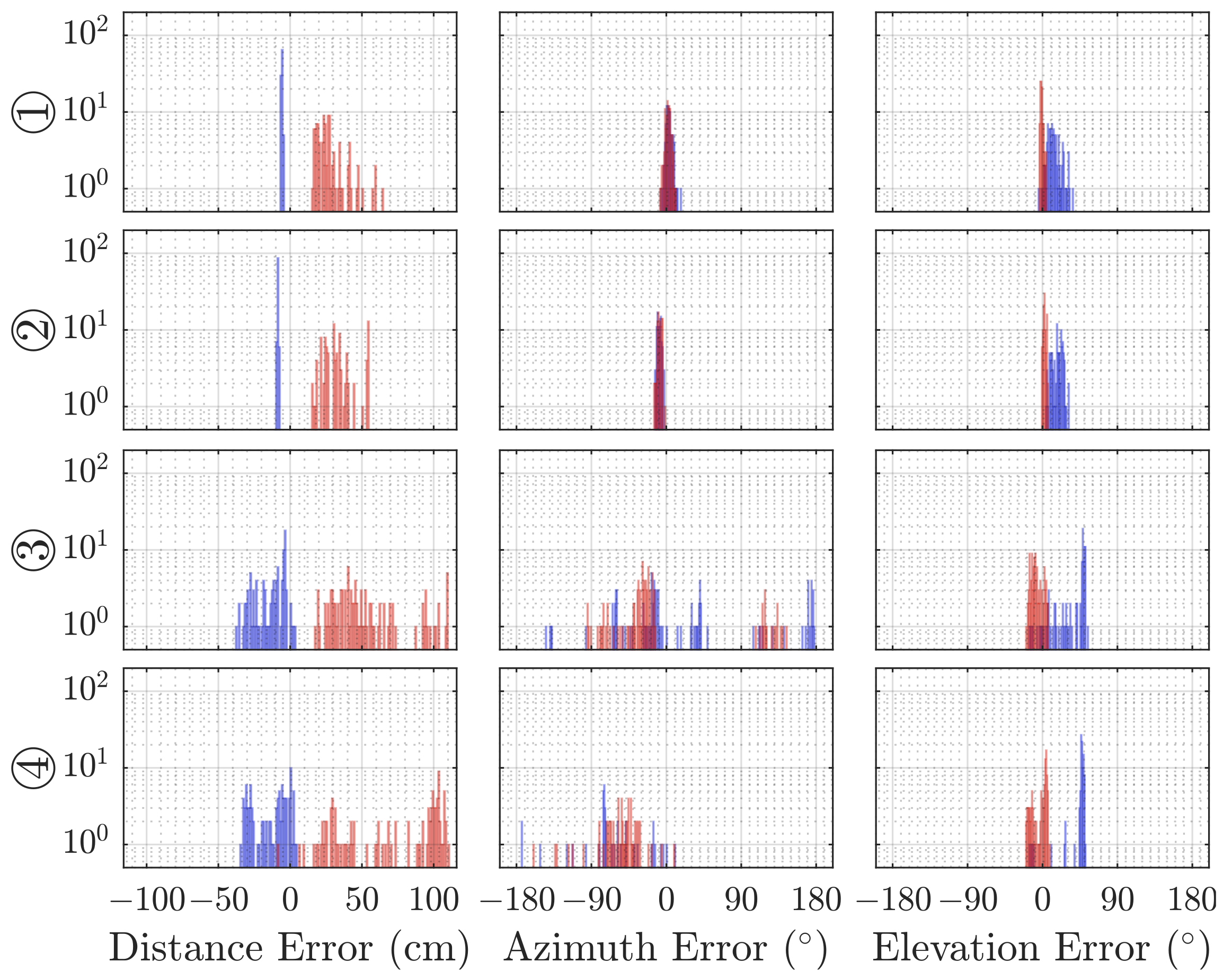
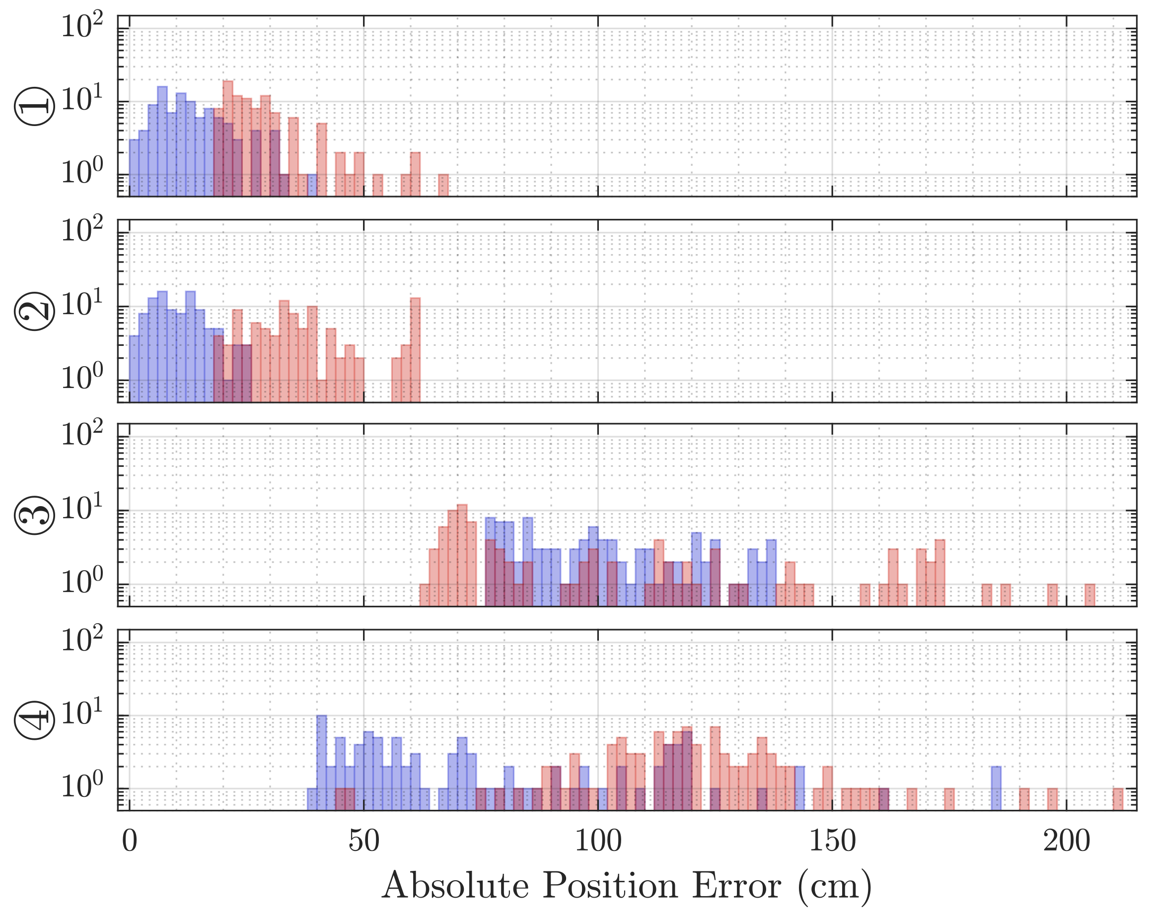
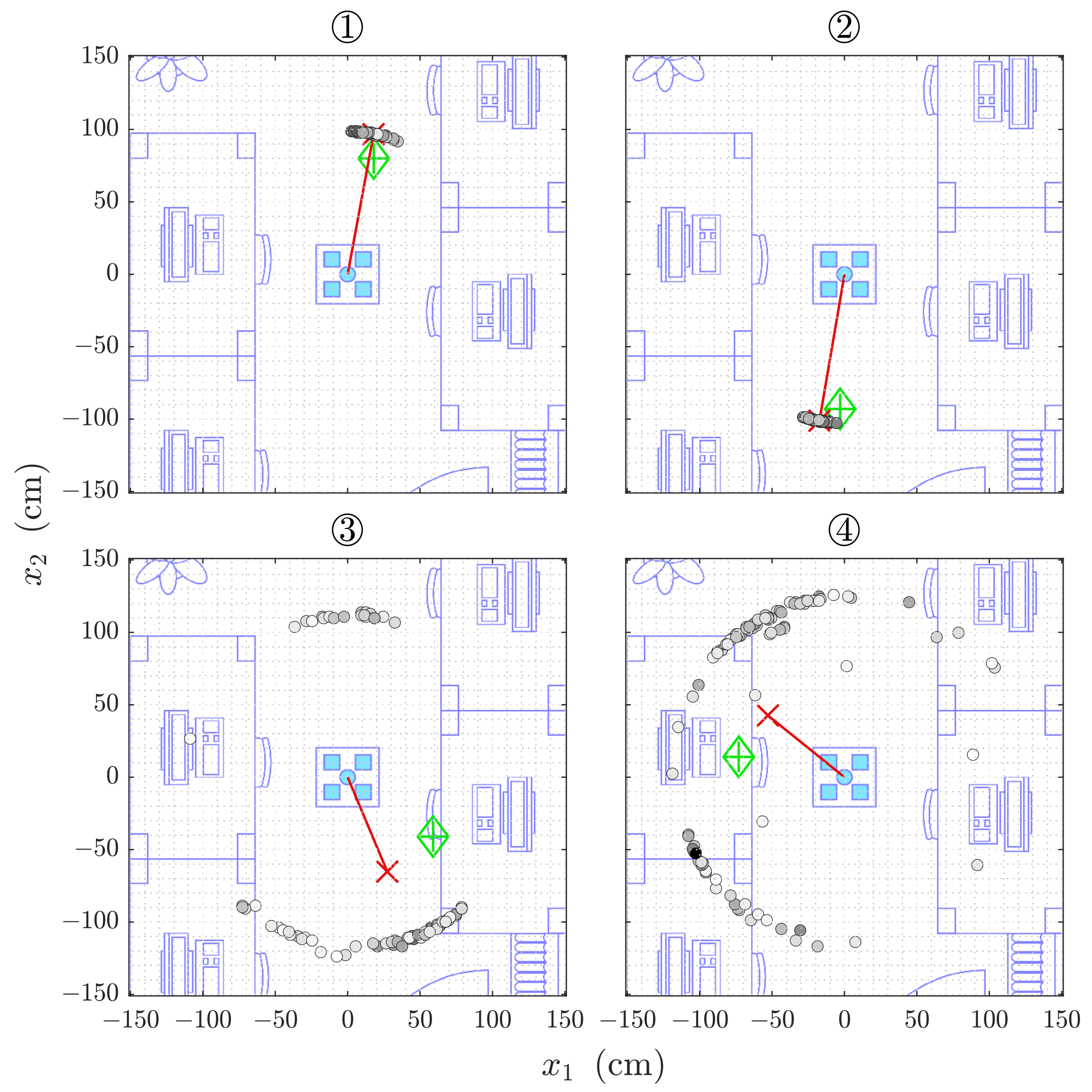
4.2.2. Direct Intersection
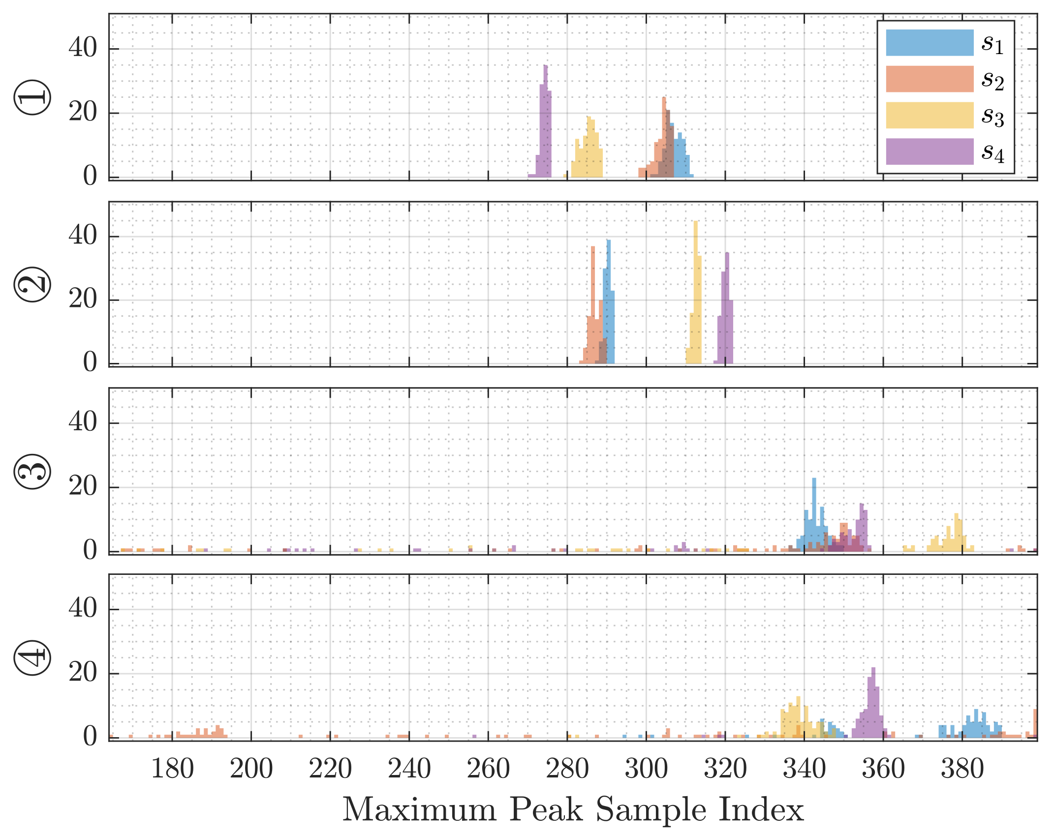
4.2.3. Sonogram
5. Discussion
5.1. Localization
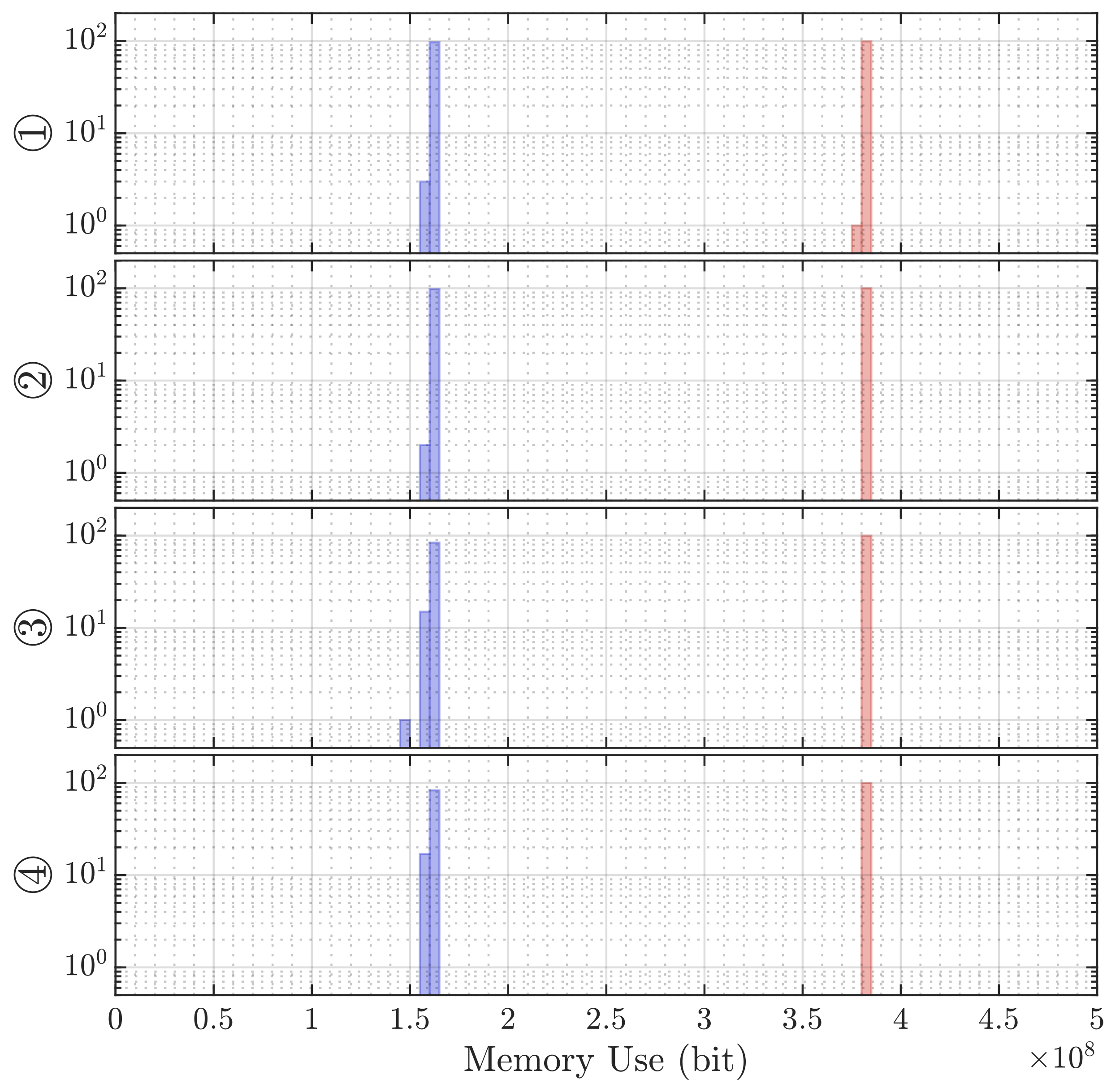
5.2. Performance
6. Conclusions
Author Contributions
Funding
Institutional Review Board Statement
Informed Consent Statement
Data Availability Statement
Acknowledgments
Conflicts of Interest
Abbreviations
| MDPI | Multidisciplinary Digital Publishing Institute |
| DI | Direct Intersection |
| DoA | Direction of Arrival |
| FMCW | Frequency-Modulated Continuous-Wave |
| LS | Least-Squares |
| RF | Radio-Frequency |
| RIR | Room Impulse Response |
| RSSI | Received Signal Strength Indicator |
| SONO | Sonogram |
| SNR | Signal-to-Noise Ratio |
| TDoA | Time Difference of Arrival |
| ToF | Time of Flight |
References
- Zafari, F.; Gkelias, A.; Leung, K.K. A Survey of Indoor Localization Systems and Technologies. IEEE Commun. Surv. Tutor. 2019, 21, 2568–2599. [Google Scholar] [CrossRef] [Green Version]
- Billa, A.; Shayea, I.; Alhammadi, A.; Abdullah, Q.; Roslee, M. An Overview of Indoor Localization Technologies: Toward IoT Navigation Services. In Proceedings of the 2020 IEEE 5th International Symposium on Telecommunication Technologies (ISTT), Shah Alam, Malaysia, 9–11 November 2020; pp. 76–81. [Google Scholar] [CrossRef]
- Obeidat, H.; Shuaieb, W.; Obeidat, O.; Abd-Alhameed, R. A Review of Indoor Localization Techniques and Wireless Technologies. Wirel. Personal Commun. 2021. [Google Scholar] [CrossRef]
- Höflinger, F.; Saphala, A.; Schott, D.J.; Reindl, L.M.; Schindelhauer, C. Passive Indoor-Localization using Echoes of Ultrasound Signals. In Proceedings of the 2019 International Conference on Advanced Information Technologies (ICAIT), Yangon, Myanmar, 6–7 November 2019; pp. 60–65. [Google Scholar] [CrossRef]
- Pirzada, N.; Nayan, M.Y.; Subhan, F.; Hassan, M.F.; Khan, M.A. Comparative analysis of active and passive indoor localization systems. AASRI Procedia 2013, 5, 92–97. [Google Scholar] [CrossRef]
- Caicedo, D.; Pandharipande, A. Distributed Ultrasonic Zoned Presence Sensing System. IEEE Sens. J. 2014, 14, 234–243. [Google Scholar] [CrossRef]
- Pandharipande, A.; Caicedo, D. User localization using ultrasonic presence sensing systems. In Proceedings of the 2012 IEEE International Conference on Systems, Man, and Cybernetics (SMC), Seoul, Korea, 14–17 October 2012; pp. 3191–3196. [Google Scholar] [CrossRef]
- Kim, K.; Choi, H. A New Approach to Power Efficiency Improvement of Ultrasonic Transmitters via a Dynamic Bias Technique. Sensors 2021, 21, 2795. [Google Scholar] [CrossRef]
- Caicedo, D.; Pandharipande, A. Transmission slot allocation and synchronization protocol for ultrasonic sensor systems. In Proceedings of the 2013 10th IEEE International Conference on Networking, Sensing and Control (ICNSC), Evry, France, 10–12 April 2013; pp. 288–293. [Google Scholar] [CrossRef]
- Carotenuto, R.; Merenda, M.; Iero, D.; Della Corte, F.G. An Indoor Ultrasonic System for Autonomous 3-D Positioning. IEEE Trans. Instrum. Meas. 2019, 68, 2507–2518. [Google Scholar] [CrossRef]
- Patwari, N.; Ash, J.; Kyperountas, S.; Hero, A.; Moses, R.; Correal, N. Locating the nodes: Cooperative localization in wireless sensor networks. IEEE Signal Process. Mag. 2005, 22, 54–69. [Google Scholar] [CrossRef]
- Kuttruff, H. Geometrical room acoustics. In Room Acoustics, 5th ed.; Spon Press, Taylor & Francis: Abingdon-on-Thames, UK, 2009. [Google Scholar]
- Zhang, S.; Ma, X.; Dong, Z.; Zhou, W. Ultrasonic Spatial Target Localization Using Artificial Pinnae of Brown Long-eared Bat. bioRxiv 2020. [Google Scholar] [CrossRef] [Green Version]
- Kosba, A.E.; Saeed, A.; Youssef, M. RASID: A robust WLAN device-free passive motion detection system. In Proceedings of the 2012 IEEE International Conference on Pervasive Computing and Communications, Lugano, Switzerland, 19–23 March 2012. [Google Scholar] [CrossRef] [Green Version]
- Seshadri, V.; Zaruba, G.; Huber, M. A Bayesian sampling approach to in-door localization of wireless devices using received signal strength indication. In Proceedings of the Third IEEE International Conference on Pervasive Computing and Communications, Kauai, HI, USA, 8–12 March 2005; pp. 75–84. [Google Scholar] [CrossRef] [Green Version]
- Wang, G.; Gu, C.; Inoue, T.; Li, C. A Hybrid FMCW-Interferometry Radar for Indoor Precise Positioning and Versatile Life Activity Monitoring. IEEE Trans. Microw. Theory Tech. 2014, 62, 2812–2822. [Google Scholar] [CrossRef]
- Bordoy, J.; Schott, D.J.; Xie, J.; Bannoura, A.; Klein, P.; Striet, L.; Höflinger, F.; Häring, I.; Reindl, L.; Schindelhauer, C. Acoustic Indoor Localization Augmentation by Self-Calibration and Machine Learning. Sensors 2020, 20, 1177. [Google Scholar] [CrossRef] [Green Version]
- Pullano, S.A.; Bianco, M.G.; Critello, D.C.; Menniti, M.; La Gatta, A.; Fiorillo, A.S. A Recursive Algorithm for Indoor Positioning Using Pulse-Echo Ultrasonic Signals. Sensors 2020, 20, 5042. [Google Scholar] [CrossRef]
- Schott, D.J.; Faisal, M.; Höflinger, F.; Reindl, L.M.; Bordoy Andreú, J.; Schindelhauer, C. Underwater localization utilizing a modified acoustic indoor tracking system. In Proceedings of the 2017 IEEE 7th International Conference on Underwater System Technology: Theory and Applications (USYS), Kuala Lumpur, Malaysia, 18–20 December 2017. [Google Scholar] [CrossRef]
- Chang, S.; Li, Y.; He, Y.; Wang, H. Target Localization in Underwater Acoustic Sensor Networks Using RSS Measurements. Appl. Sci. 2018, 8, 225. [Google Scholar] [CrossRef] [Green Version]
- Cobos, M.; Antonacci, F.; Alexandridis, A.; Mouchtaris, A.; Lee, B. A Survey of Sound Source Localization Methods in Wireless Acoustic Sensor Networks. Wirel. Commun. Mob. Comput. 2017, 2017, 3956282. [Google Scholar] [CrossRef]
- Hage, S.R.; Metzner, W. Potential effects of anthropogenic noise on echolocation behavior in horseshoe bats. Commun. Integr. Biol. 2013, 6, e24753. [Google Scholar] [CrossRef]
- Rahman, A.B.M.M.; Li, T.; Wang, Y. Recent Advances in Indoor Localization via Visible Lights: A Survey. Sensors 2020, 20, 1382. [Google Scholar] [CrossRef] [PubMed] [Green Version]
- Mrazovac, B.; Bjelica, M.; Kukolj, D.; Todorovic, B.; Samardzija, D. A human detection method for residential smart energy systems based on Zigbee RSSI changes. IEEE Trans. Consum. Electron. 2012, 58, 819–824. [Google Scholar] [CrossRef]
- Gunasagaran, R.; Kamarudin, L.M.; Zakaria, A. Wi-Fi For Indoor Device Free Passive Localization (DfPL): An Overview. Indones. J. Electr. Eng. Inform. (IJEEI) 2020, 8. [Google Scholar] [CrossRef]
- Retscher, G.; Leb, A. Development of a Smartphone-Based University Library Navigation and Information Service Employing Wi-Fi Location Fingerprinting. Sensors 2021, 21, 432. [Google Scholar] [CrossRef]
- Kaltiokallio, O.; Bocca, M. Real-Time Intrusion Detection and Tracking in Indoor Environment through Distributed RSSI Processing. In Proceedings of the 2011 IEEE 17th International Conference on Embedded and Real-Time Computing Systems and Applications, Toyama, Japan, 28–31 August 2011. [Google Scholar] [CrossRef]
- Yigitler, H.; Jantti, R.; Kaltiokallio, O.; Patwari, N. Detector Based Radio Tomographic Imaging. IEEE Trans. Mob. Comput. 2018, 17, 58–71. [Google Scholar] [CrossRef]
- Hillyard, P.; Patwari, N.; Daruki, S.; Venkatasubramanian, S. You’re crossing the line: Localizing border crossings using wireless RF links. In Proceedings of the 2015 IEEE Signal Processing and Signal Processing Education Workshop (SP/SPE), Salt Lake City, UT, USA, 9–12 August 2015. [Google Scholar] [CrossRef]
- Suijker, E.M.; Bolt, R.J.; van Wanum, M.; van Heijningen, M.; Maas, A.P.M.; van Vliet, F.E. Low cost low power 24 GHz FMCW Radar transceiver for indoor presence detection. In Proceedings of the 2014 44th European Microwave Conference, Rome, Italy, 6–9 October 2014; pp. 1758–1761. [Google Scholar] [CrossRef] [Green Version]
- Del Hougne, P.; Imani, M.F.; Fink, M.; Smith, D.R.; Lerosey, G. Precise Localization of Multiple Noncooperative Objects in a Disordered Cavity by Wave Front Shaping. Phys. Rev. Lett. 2018, 121, 063901. [Google Scholar] [CrossRef] [Green Version]
- Del Hougne, M.; Gigan, S.; del Hougne, P. Deeply Sub-Wavelength Localization with Reverberation-Coded-Aperture. arXiv 2021, arXiv:2102.05642. [Google Scholar]
- Hnat, T.W.; Griffiths, E.; Dawson, R.; Whitehouse, K. Doorjamb: Unobtrusive room-level tracking of people in homes using doorway sensors. In Proceedings of the The 10th ACM Conference on Embedded Network Sensor Systems (SenSys 2012), Toronto, ON, Canada, 6–9 November 2012. [Google Scholar] [CrossRef]
- Caicedo, D.; Pandharipande, A. Ultrasonic array sensor for indoor presence detection. In Proceedings of the 2012 20th European Signal Processing Conference (EUSIPCO), Bucharest, Romania, 27–31 August 2012; pp. 175–179. [Google Scholar]
- Nishida, Y.; Murakami, S.; Hori, T.; Mizoguchi, H. Minimally privacy-violative human location sensor by ultrasonic Radar embedded on ceiling. In Proceedings of the 2004 IEEE Sensors, Vienna, Austria, 24–27 October 2004. [Google Scholar] [CrossRef]
- Bordoy, J.; Wendeberg, J.; Schindelhauer, C.; Reindl, L.M. Single transceiver device-free indoor localization using ultrasound body reflections and walls. In Proceedings of the 2015 International Conference on Indoor Positioning and Indoor Navigation (IPIN), Banff, AB, Canada, 13–16 October 2015. [Google Scholar] [CrossRef]
- Mokhtari, G.; Zhang, Q.; Nourbakhsh, G.; Ball, S.; Karunanithi, M. BLUESOUND: A New Resident Identification Sensor—Using Ultrasound Array and BLE Technology for Smart Home Platform. IEEE Sens. J. 2017, 17, 1503–1512. [Google Scholar] [CrossRef]
- Nowakowski, T.; de Rosny, J.; Daudet, L. Robust source localization from wavefield separation including prior information. J. Acoust. Soc. Am. 2017, 141, 2375–2386. [Google Scholar] [CrossRef] [PubMed]
- Conti, S.G.; de Rosny, J.; Roux, P.; Demer, D.A. Characterization of scatterer motion in a reverberant medium. J. Acoust. Soc. Am. 2006, 119, 769. [Google Scholar] [CrossRef] [Green Version]
- Conti, S.G.; Roux, P.; Demer, D.A.; de Rosny, J. Measurements of the total scattering and absorption cross-sections of the human body. J. Acoust. Soc. Am. 2003, 114, 2357. [Google Scholar] [CrossRef]
- Ribeiro, F.; Florencio, D.; Ba, D.; Zhang, C. Geometrically Constrained Room Modeling With Compact Microphone Arrays. IEEE Trans. Audio Speech Lang. Process. 2012, 20, 1449–1460. [Google Scholar] [CrossRef]
- Steckel, J.; Boen, A.; Peremans, H. Broadband 3-D Sonar System Using a Sparse Array for Indoor Navigation. IEEE Trans. Robot. 2013, 29, 161–171. [Google Scholar] [CrossRef]
- Steckel, J. Sonar System Combining an Emitter Array With a Sparse Receiver Array for Air-Coupled Applications. IEEE Sens. J. 2015, 15, 3446–3452. [Google Scholar] [CrossRef]
- Rajai, P.; Straeten, M.; Alirezaee, S.; Ahamed, M.J. Binaural Sonar System for Simultaneous Sensing of Distance and Direction of Extended Barriers. IEEE Sens. J. 2019, 19, 12040–12049. [Google Scholar] [CrossRef]
- Zhou, B.; Elbadry, M.; Gao, R.; Ye, F. Towards Scalable Indoor Map Construction and Refinement using Acoustics on Smartphones. IEEE Trans. Mob. Comput. 2020, 19, 217–230. [Google Scholar] [CrossRef]
- Bordoy, J.; Schindelhauer, C.; Hoeflinger, F.; Reindl, L.M. Exploiting Acoustic Echoes for Smartphone Localization and Microphone Self-Calibration. IEEE Trans. Instrum. Meas. 2019, 69, 1484–1492. [Google Scholar] [CrossRef]
- Kundu, T. Acoustic source localization. Ultrasonics 2014, 54, 25–38. [Google Scholar] [CrossRef] [PubMed]
- Liu, C.; Wu, K.; He, T. Sensor localization with Ring Overlapping based on Comparison of Received Signal Strength Indicator. In Proceedings of the 2004 IEEE International Conference on Mobile Ad-hoc and Sensor Systems, Fort Lauderdale, FL, USA, 25–27 October 2004. [Google Scholar] [CrossRef]
- Dmochowski, J.P.; Benesty, J.; Affes, S. A Generalized Steered Response Power Method for Computationally Viable Source Localization. IEEE Trans. Audio Speech Lang. Process. 2007, 15, 2510–2526. [Google Scholar] [CrossRef]
- Cook, C. Pulse Compression-Key to More Efficient Radar Transmission. Proc. IRE 1960, 48, 310–316. [Google Scholar] [CrossRef]
- Springer, A.; Gugler, W.; Huemer, M.; Reindl, L.; Ruppel, C.C.W.; Weigel, R. Spread spectrum communications using chirp signals. In Proceedings of the IEEE/AFCEA EUROCOMM 2000. Information Systems for Enhanced Public Safety and Security, Munich, Germany, 19 May 2000; pp. 166–170. [Google Scholar] [CrossRef]
- Milewski, A.; Sedek, E.; Gawor, S. Amplitude Weighting of Linear Frequency Modulated Chirp Signals. In Proceedings of the 2007 IEEE 15th Signal Processing and Communications Applications, Eskisehir, Turkey, 11–13 June 2007; pp. 383–386. [Google Scholar] [CrossRef]
- Carotenuto, R.; Merenda, M.; Iero, D.; G. Della Corte, F. Simulating Signal Aberration and Ranging Error for Ultrasonic Indoor Positioning. Sensors 2020, 20, 3548. [Google Scholar] [CrossRef] [PubMed]
- Schnitzler, H.U.; Kalko, E.K.V. Echolocation by Insect-Eating Bats: We define four distinct functional groups of bats and find differences in signal structure that correlate with the typical echolocation tasks faced by each group. BioScience 2001, 51, 557–569. [Google Scholar] [CrossRef]
- Saphala, A. Design and Implementation of Acoustic Phased Array for In-Air Presence Detection. Master’s Thesis, Faculty of Engineering, University of Freiburg, Freiburg, Germany, 2019. [Google Scholar]
- MathWorks. ismember. Available online: https://de.mathworks.com/help/matlab/ref/double.ismember.html (accessed on 27 May 2021).
- MathWorks. ind2sub. Available online: https://www.mathworks.com/help/matlab/ref/ind2sub.html (accessed on 27 May 2021).
- MathWorks. smooth. Available online: https://de.mathworks.com/help/curvefit/smooth.html (accessed on 27 May 2021).
- MathWorks. find. Available online: https://de.mathworks.com/help/matlab/ref/find.html (accessed on 27 May 2021).
- Dylan Mikesell, T.; van Wijk, K.; Blum, T.E.; Snieder, R.; Sato, H. Analyzing the coda from correlating scattered surface waves. J. Acoust. Soc. Am. 2012, 131, EL275–EL281. [Google Scholar] [CrossRef] [PubMed] [Green Version]
- Kuttruff, H. Decaying modes, reverberation. In Room Acoustics, 5th ed.; Spon Press, Taylor & Francis: Abingdon-on-Thames, UK, 2009. [Google Scholar]
- Lerch, R.; Sessler, G.M.; Wolf, D. Statistische Raumakustik. In Technische Akustik, 1st ed.; Springer: Berlin/Heidelberg, Germany, 2009. [Google Scholar] [CrossRef]
- Lerch, R.; Sessler, G.M.; Wolf, D. Wellentheoretische Raumakustik. In Technische Akustik, 1st ed.; Springer: Berlin/Heidelberg, Germany, 2009. [Google Scholar] [CrossRef]
- Kuttruff, H. Steady-state sound field. In Room Acoustics, 5th ed.; Spon Press Taylor & Francis: Abingdon-on-Thames, UK, 2009. [Google Scholar]


| Position | r (m) | () | () |
|---|---|---|---|
| ① | 1.58 | 77 | 59 |
| ② | 1.70 | −92 | 57 |
| ③ | 1.23 | −35 | 54 |
| ④ | 1.26 | 169 | 54 |
| Position | r (m) | () | () |
|---|---|---|---|
| ① | 1.83 ± 0.14 | 81 ± 4 | 61 ± 1 |
| ② | 2.01 ± 0.11 | −100 ± 3 | 61 ± 1 |
| ③ | 1.92 ± 0.37 | 4 ± 96 | 59 ± 4 |
| ④ | 2.12 ± 0.25 | −58 ± 135 | 60 ± 3 |
| Position | r (m) | () | () |
|---|---|---|---|
| ① | 1.85 ± 0.10 | 80 ± 4 | 58 ± 2 |
| ② | 2.03 ± 0.11 | −100 ± 3 | 60 ± 2 |
| ③ | 1.77 ± 0.26 | −41 ± 69 | 47 ± 7 |
| ④ | 1.96 ± 0.34 | 31 ± 119 | 51 ± 9 |
| Direct Intersection | Sonogram | |||||
|---|---|---|---|---|---|---|
| Position | (m) | () | () | (m) | () | () |
| ① | 0.25 | 3 | 2 | 0.27 | 2 | 1 |
| ② | 0.31 | 8 | 4 | 0.34 | 8 | 3 |
| ③ | 0.69 | 39 | 5 | 0.53 | 6 | 7 |
| ④ | 0.87 | 47 | 6 | 0.70 | 138 | 3 |
| Direct Intersection | Sonogram | |
|---|---|---|
| Position | Time (s) | Time (s) |
| ① | 0.94 ± 0.17 | 1.14 ± 0.07 |
| ② | 0.66 ± 0.13 | 1.20 ± 0.02 |
| ③ | 6.38 ± 6.60 | 1.10 ± 0.01 |
| ④ | 8.58 ± 7.12 | 1.10 ± 0.01 |
| Direct Intersection | Sonogram |
|---|---|
| 1.600 ± 0.004 | 3.840 ± 0.002 |
Publisher’s Note: MDPI stays neutral with regard to jurisdictional claims in published maps and institutional affiliations. |
© 2021 by the authors. Licensee MDPI, Basel, Switzerland. This article is an open access article distributed under the terms and conditions of the Creative Commons Attribution (CC BY) license (https://creativecommons.org/licenses/by/4.0/).
Share and Cite
Schott, D.J.; Saphala, A.; Fischer, G.; Xiong, W.; Gabbrielli, A.; Bordoy, J.; Höflinger, F.; Fischer, K.; Schindelhauer, C.; Rupitsch, S.J. Comparison of Direct Intersection and Sonogram Methods for Acoustic Indoor Localization of Persons. Sensors 2021, 21, 4465. https://doi.org/10.3390/s21134465
Schott DJ, Saphala A, Fischer G, Xiong W, Gabbrielli A, Bordoy J, Höflinger F, Fischer K, Schindelhauer C, Rupitsch SJ. Comparison of Direct Intersection and Sonogram Methods for Acoustic Indoor Localization of Persons. Sensors. 2021; 21(13):4465. https://doi.org/10.3390/s21134465
Chicago/Turabian StyleSchott, Dominik Jan, Addythia Saphala, Georg Fischer, Wenxin Xiong, Andrea Gabbrielli, Joan Bordoy, Fabian Höflinger, Kai Fischer, Christian Schindelhauer, and Stefan Johann Rupitsch. 2021. "Comparison of Direct Intersection and Sonogram Methods for Acoustic Indoor Localization of Persons" Sensors 21, no. 13: 4465. https://doi.org/10.3390/s21134465
APA StyleSchott, D. J., Saphala, A., Fischer, G., Xiong, W., Gabbrielli, A., Bordoy, J., Höflinger, F., Fischer, K., Schindelhauer, C., & Rupitsch, S. J. (2021). Comparison of Direct Intersection and Sonogram Methods for Acoustic Indoor Localization of Persons. Sensors, 21(13), 4465. https://doi.org/10.3390/s21134465