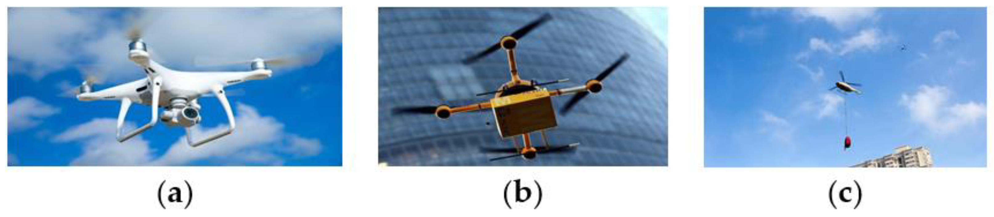
Figure 1.
The three major types of UAVs that are experiencing expanded use in the UAVs industry: (a) consumer UAVs, (b) commercial UAVs, and (c) government UAVs.
Figure 1.
The three major types of UAVs that are experiencing expanded use in the UAVs industry: (a) consumer UAVs, (b) commercial UAVs, and (c) government UAVs.
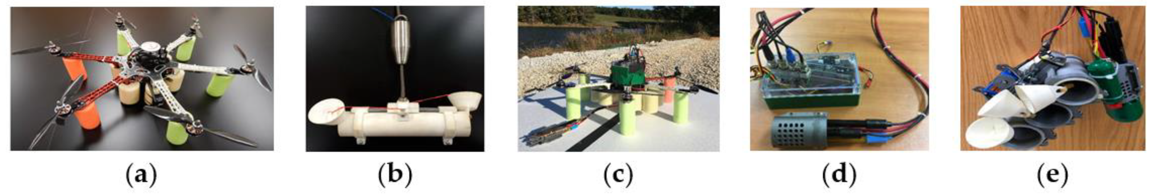
Figure 2.
From 2016 to 2020, Koparan et al designed and improved an UAV and its accessories for water quality detection: (a) water quality sampling UAV, (b) water intake device, (c) improved UAV, (d) improved sensor array, and (e) customized sensor.
Figure 2.
From 2016 to 2020, Koparan et al designed and improved an UAV and its accessories for water quality detection: (a) water quality sampling UAV, (b) water intake device, (c) improved UAV, (d) improved sensor array, and (e) customized sensor.
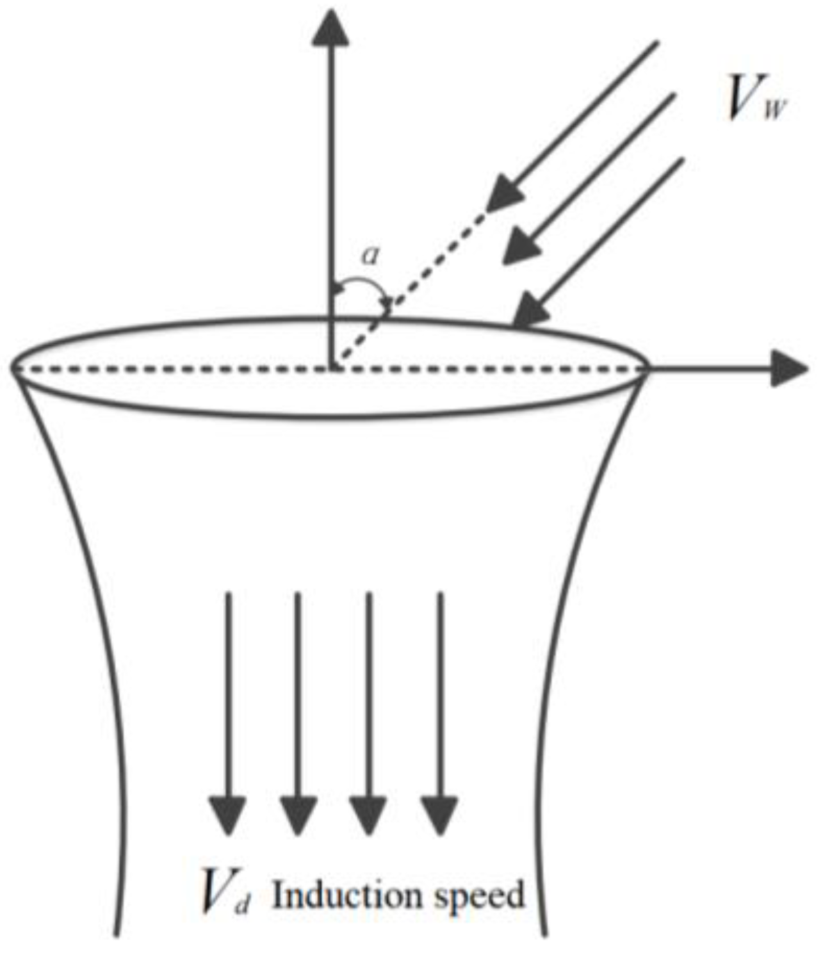
Figure 3.
Schematic diagram of the propeller slipstream flow field.
Figure 3.
Schematic diagram of the propeller slipstream flow field.
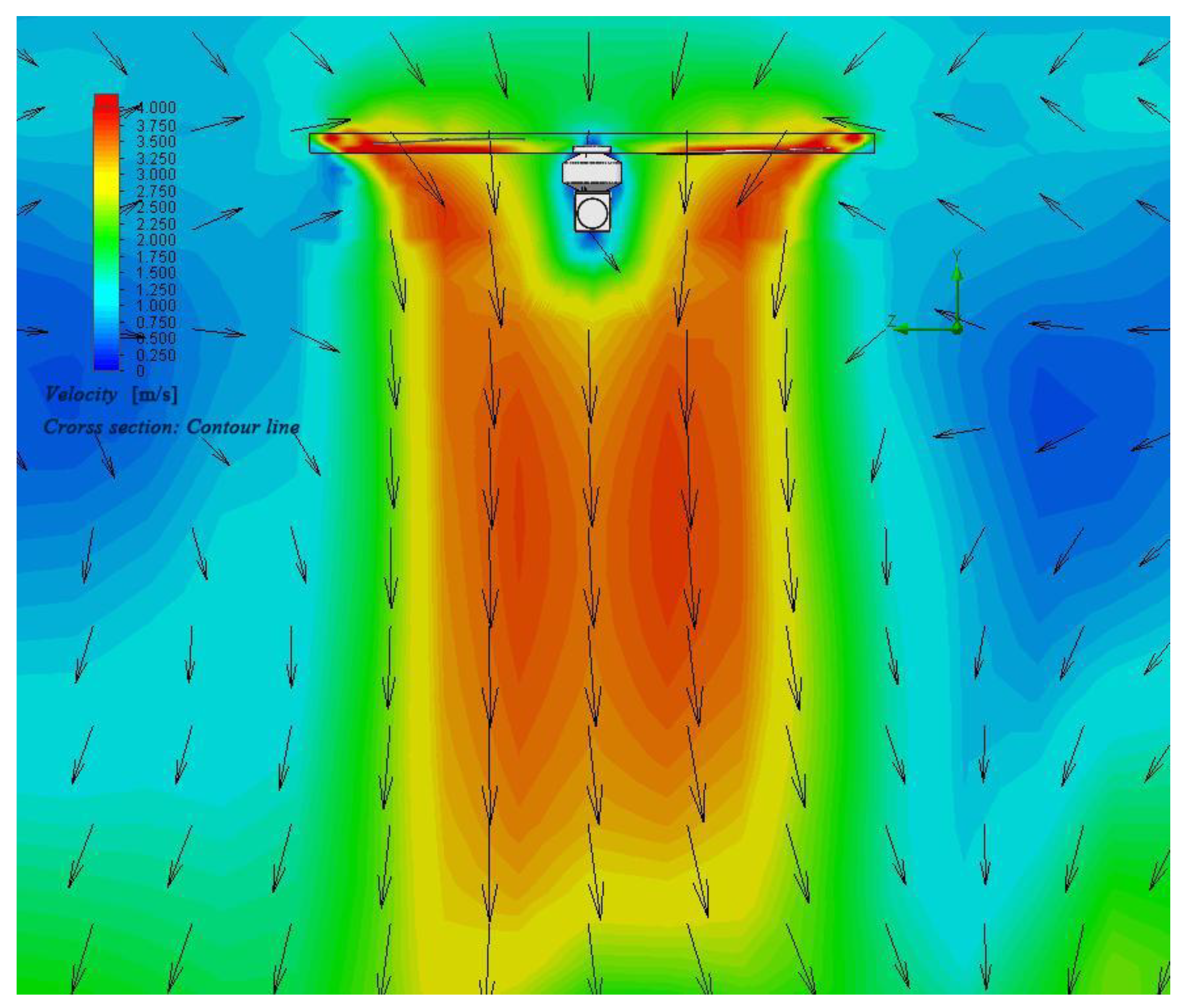
Figure 4.
The approximate simulation diagram of the slipstream flow field profile of a single rotor in hovering state.
Figure 4.
The approximate simulation diagram of the slipstream flow field profile of a single rotor in hovering state.
Figure 5.
The front and side views of a single rotor.
Figure 5.
The front and side views of a single rotor.
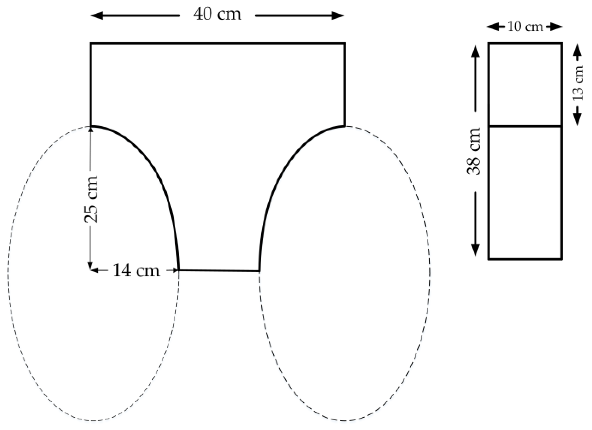
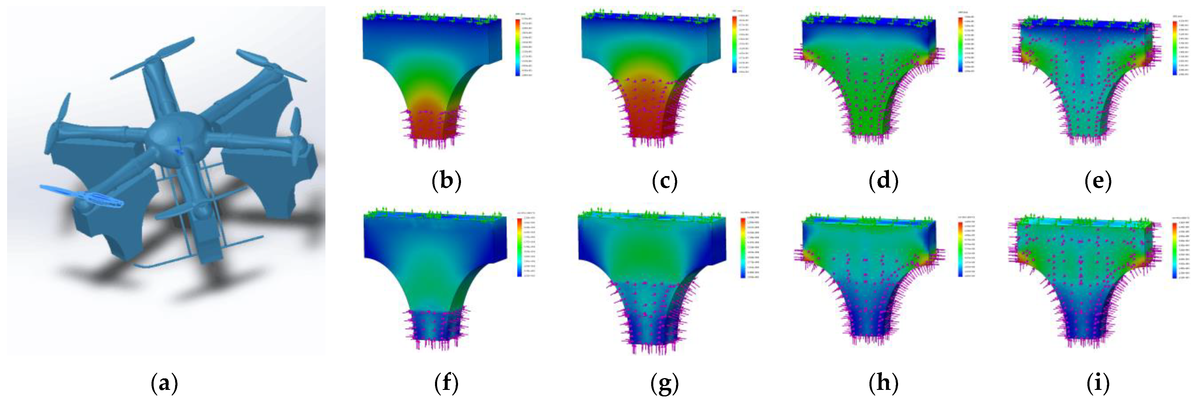
Figure 6.
Simulation analysis diagram of the floating structure. (a) 3D modeling drawing in SolidWorks; (b) deformation simulation at 10 cm immersion depth; (c) deformation simulation at 20 cm immersion depth; (d) deformation simulation at 30 cm immersion depth; (e) deformation simulation at 38 cm immersion depth; (f) pressure simulation at 10 cm immersion depth; (g) pressure simulation at 20 cm immersion depth; (h) pressure simulation at 30 cm immersion depth; and (i) pressure simulation at 38 cm immersion depth.
Figure 7.
Mathematical model of floating structure and physical map: (a) function curve determined in MATLAB; (b) mathematical model; and (c) image of the floating UAV.
Figure 7.
Mathematical model of floating structure and physical map: (a) function curve determined in MATLAB; (b) mathematical model; and (c) image of the floating UAV.
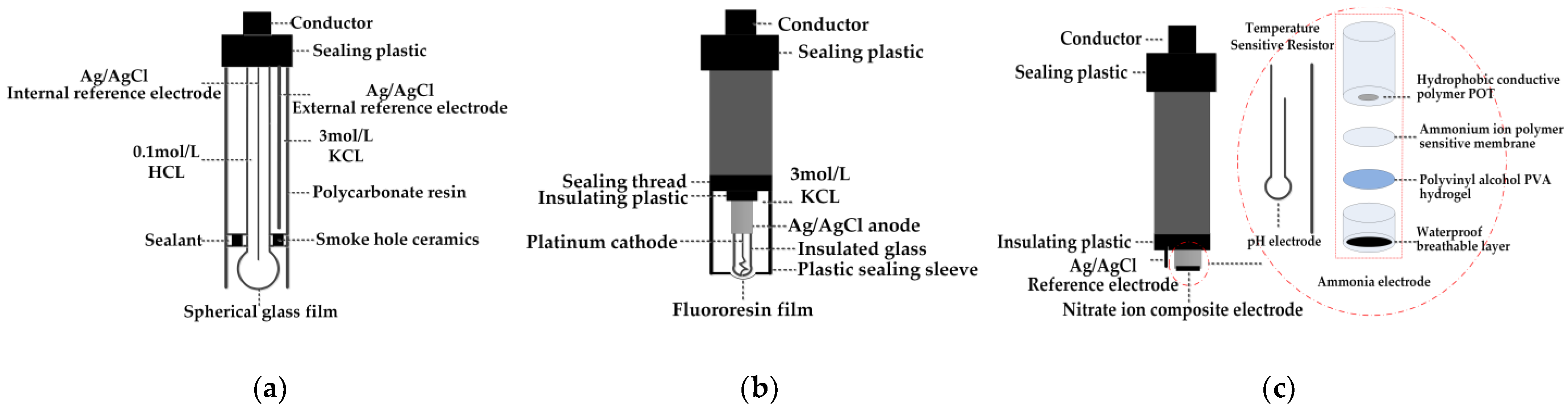
Figure 8.
Structure diagram of three parameter sensors: (a) pH composite electrode; (b) dissolved oxygen composite electrode; and (c) ammonia nitrogen composite electrode.
Figure 8.
Structure diagram of three parameter sensors: (a) pH composite electrode; (b) dissolved oxygen composite electrode; and (c) ammonia nitrogen composite electrode.
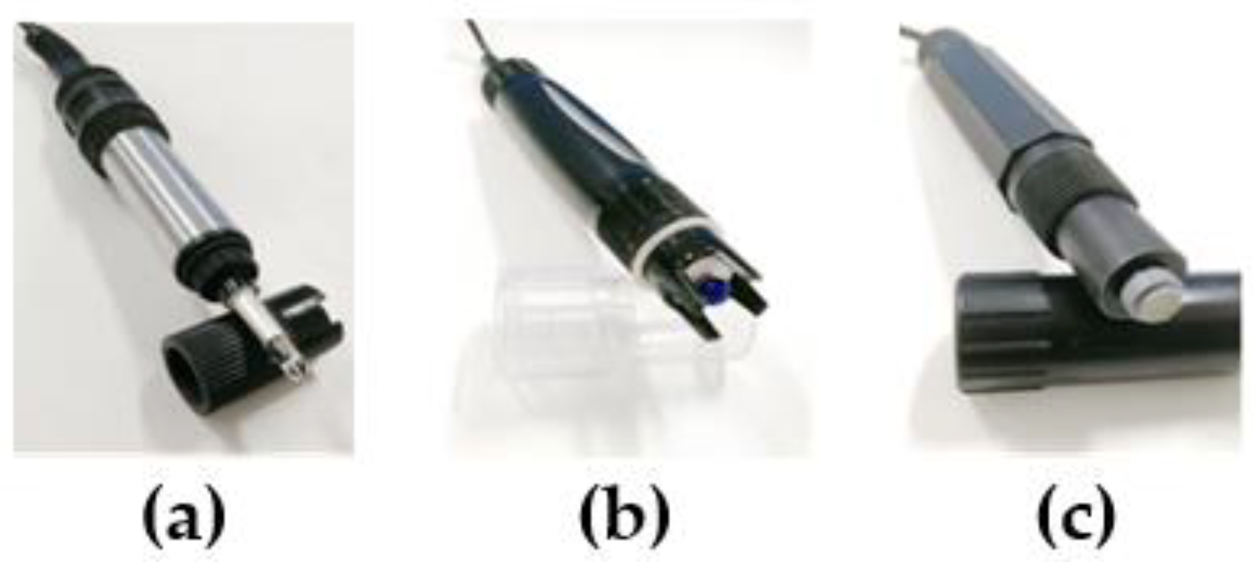
Figure 9.
Electrode-type water quality sensor probe: (a) pH probe; (b) dissolved oxygen probe; (c) and ammonia nitrogen probe.
Figure 9.
Electrode-type water quality sensor probe: (a) pH probe; (b) dissolved oxygen probe; (c) and ammonia nitrogen probe.
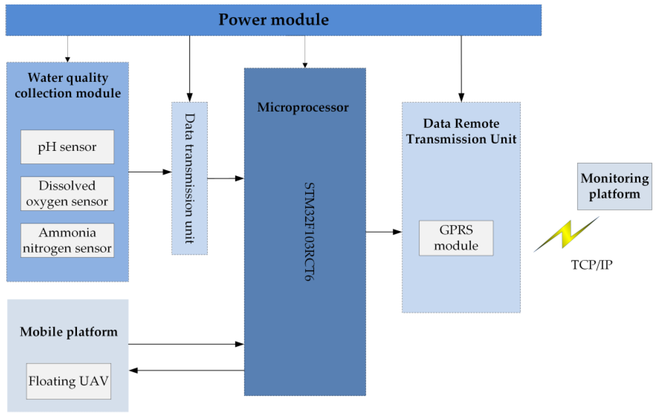
Figure 10.
Block diagram of water quality monitoring hardware module.
Figure 10.
Block diagram of water quality monitoring hardware module.
Figure 11.
Data transmission processing unit. (a) The physical diagram of the hardware; (b) the physical diagram of the data transmission processing unit.
Figure 11.
Data transmission processing unit. (a) The physical diagram of the hardware; (b) the physical diagram of the data transmission processing unit.
Figure 12.
The overall design content of the water quality monitoring system software.
Figure 12.
The overall design content of the water quality monitoring system software.
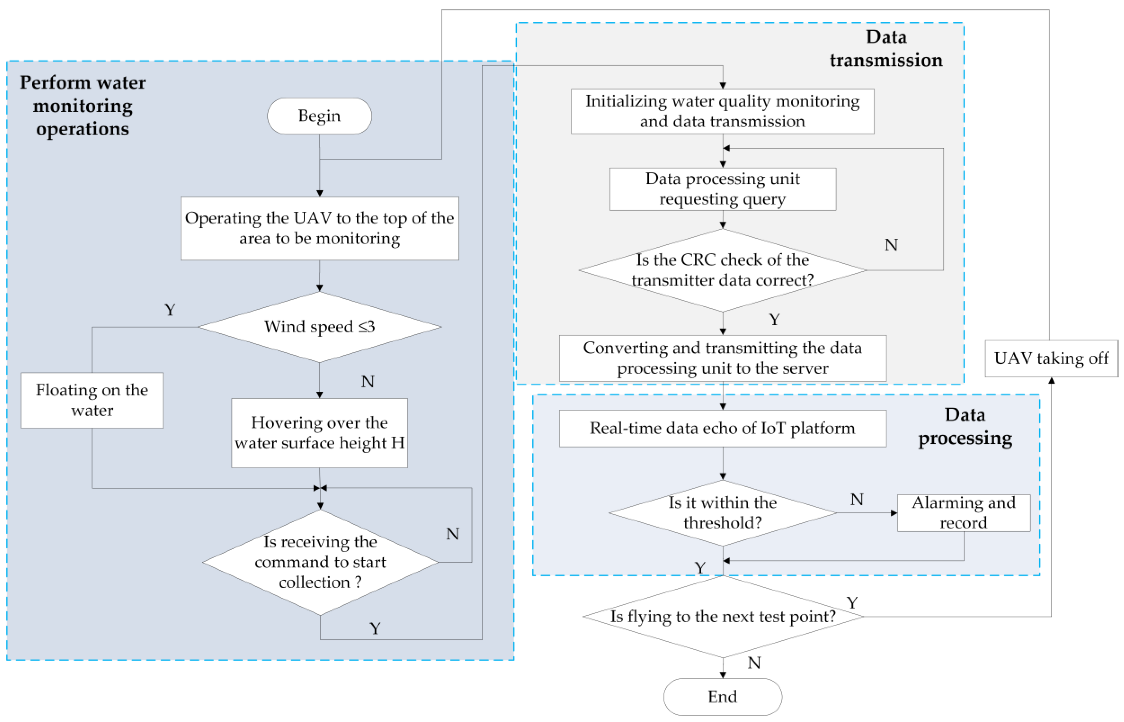
Figure 13.
Flow chart of data collection using a UAV.
Figure 13.
Flow chart of data collection using a UAV.
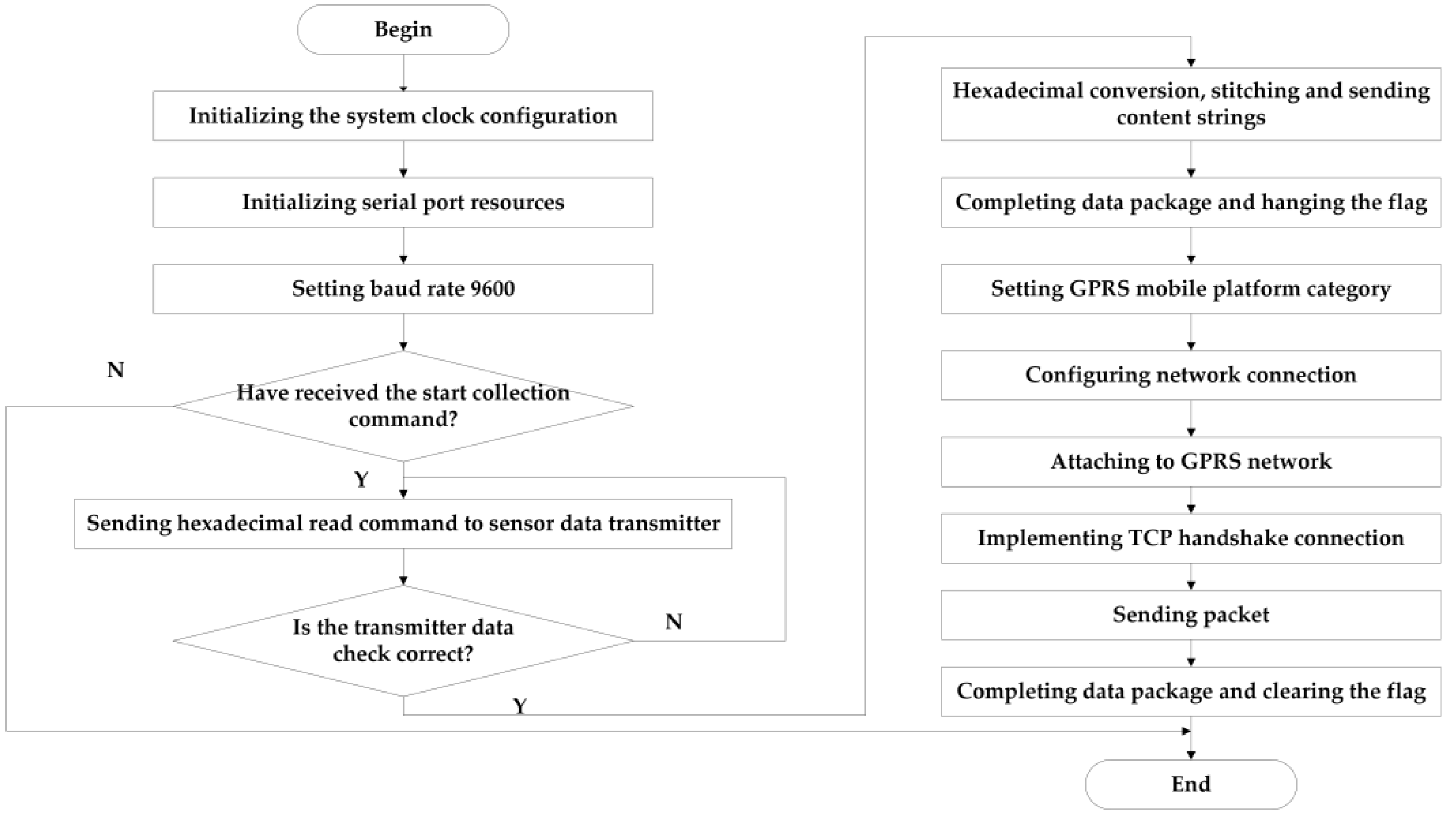
Figure 14.
Remote data transmission flowchart.
Figure 14.
Remote data transmission flowchart.
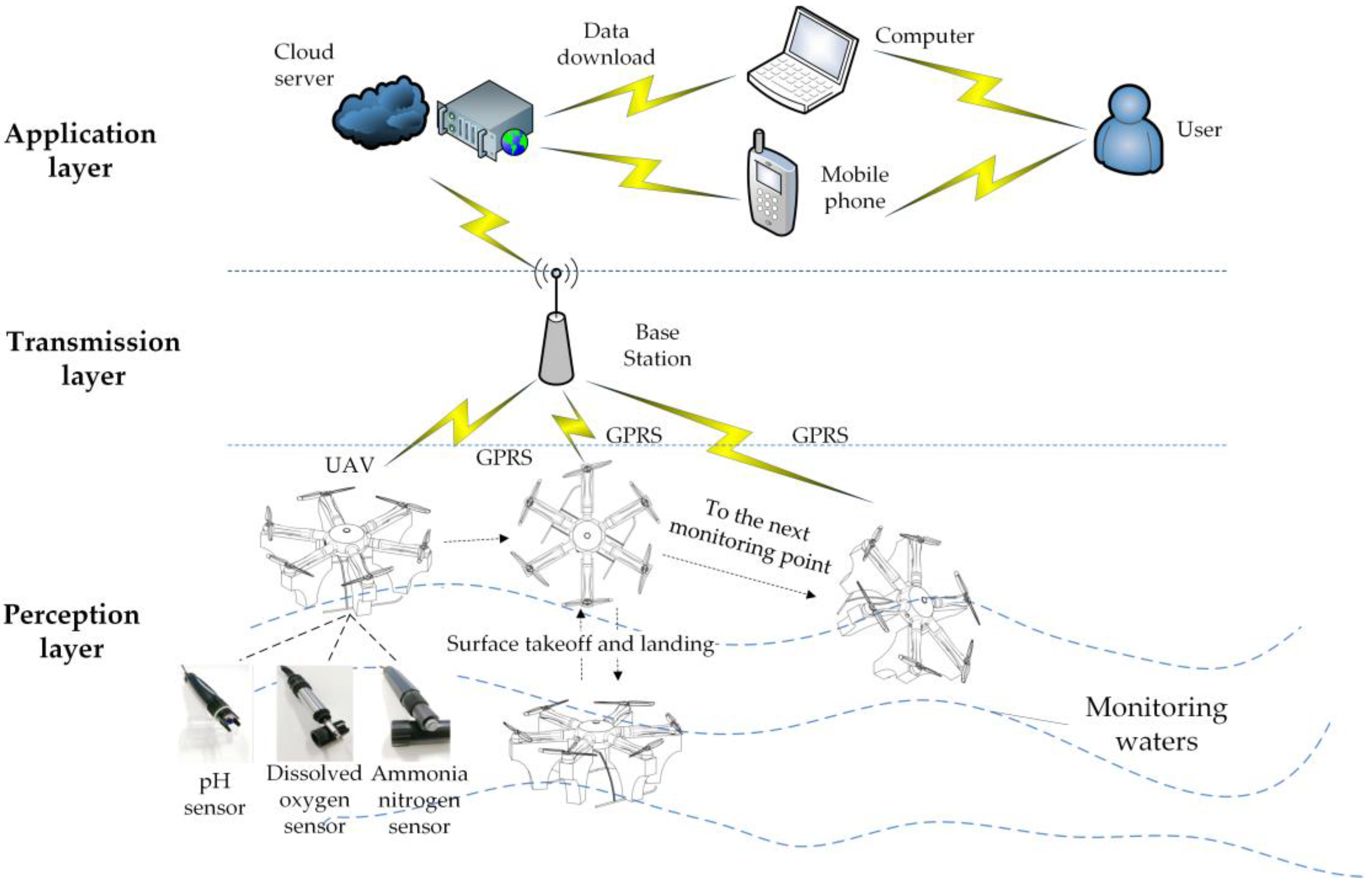
Figure 15.
Schematic diagram of UAV water quality collection and transmission.
Figure 15.
Schematic diagram of UAV water quality collection and transmission.
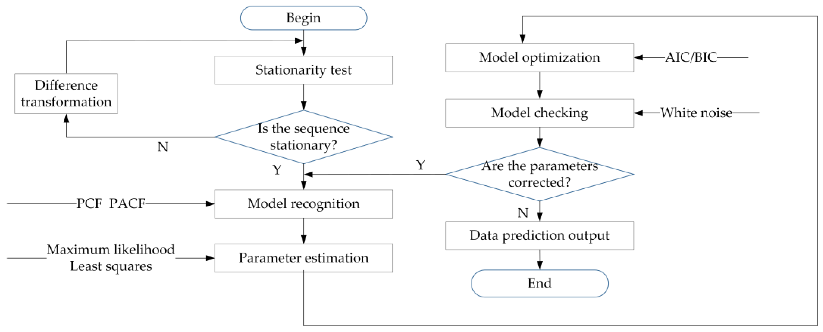
Figure 16.
Modeling flowchart based on time series analysis and prediction.
Figure 16.
Modeling flowchart based on time series analysis and prediction.
Figure 17.
The flow chart of fuzzy neural network water quality evaluation.
Figure 17.
The flow chart of fuzzy neural network water quality evaluation.
Figure 18.
Sensor array monitoring experiment of the water quality monitoring system: (a) two sets of water quality monitoring hardware and (b) a single water quality data processing unit.
Figure 18.
Sensor array monitoring experiment of the water quality monitoring system: (a) two sets of water quality monitoring hardware and (b) a single water quality data processing unit.
Figure 19.
Floating structure test diagram of a floating UAV: (a) sensor installation diagram; (b) inflatable pool test; and (c) sinking depth of the floating structure.
Figure 19.
Floating structure test diagram of a floating UAV: (a) sensor installation diagram; (b) inflatable pool test; and (c) sinking depth of the floating structure.
Figure 20.
Floating water quality monitoring UAV-fixed-point rotation and yaw flight test.
Figure 20.
Floating water quality monitoring UAV-fixed-point rotation and yaw flight test.
Figure 21.
The field experiment in Huangjia Lake: (a) takeoff on the water surface; (b) the cross-regional monitoring experiment of UAV takeoff and landing; and (c) UAV landing experiment.
Figure 21.
The field experiment in Huangjia Lake: (a) takeoff on the water surface; (b) the cross-regional monitoring experiment of UAV takeoff and landing; and (c) UAV landing experiment.
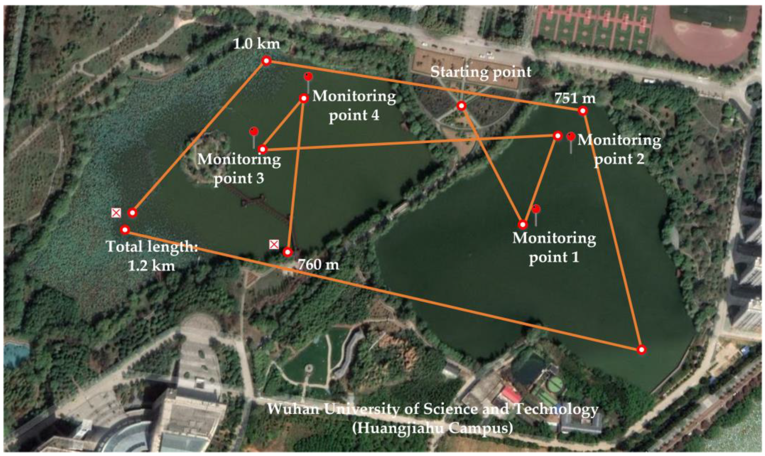
Figure 22.
UAV route map for the entire water quality monitoring process.
Figure 22.
UAV route map for the entire water quality monitoring process.
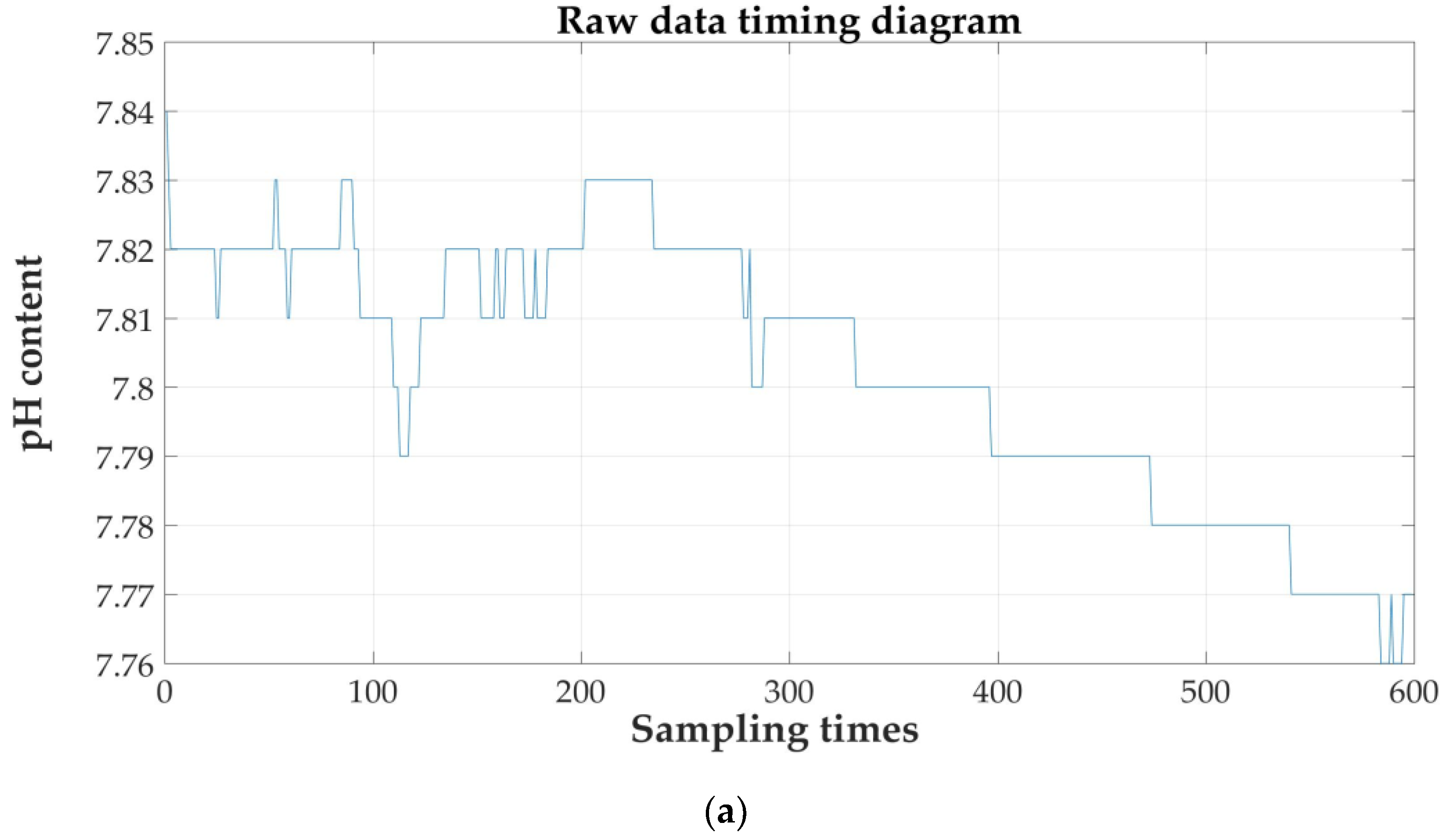
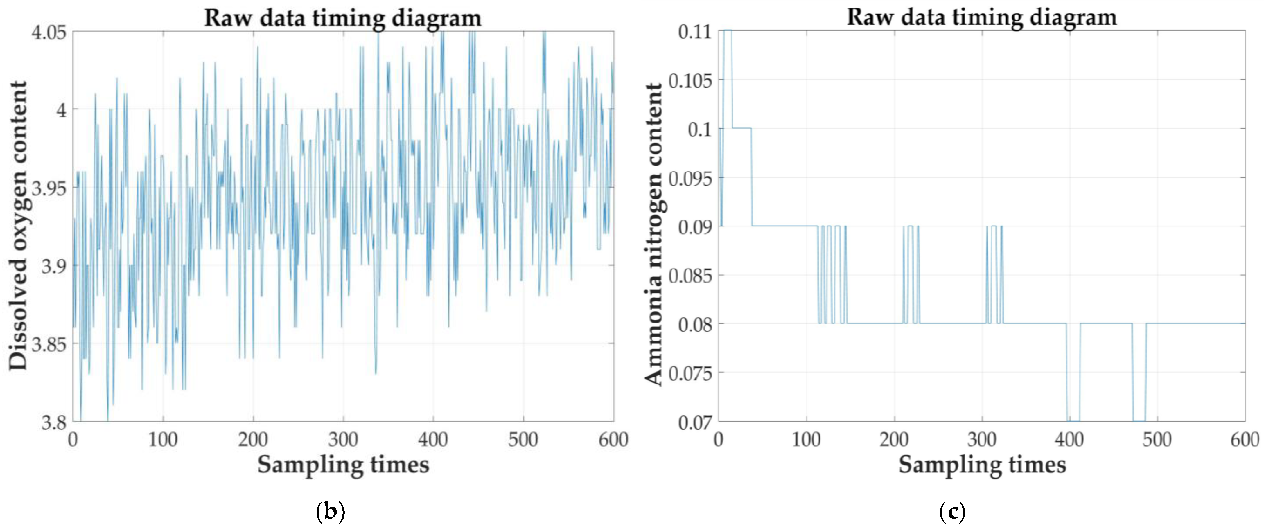
Figure 23.
Raw data timing diagram: (a) pH; (b) DO; and (c) .
Figure 23.
Raw data timing diagram: (a) pH; (b) DO; and (c) .
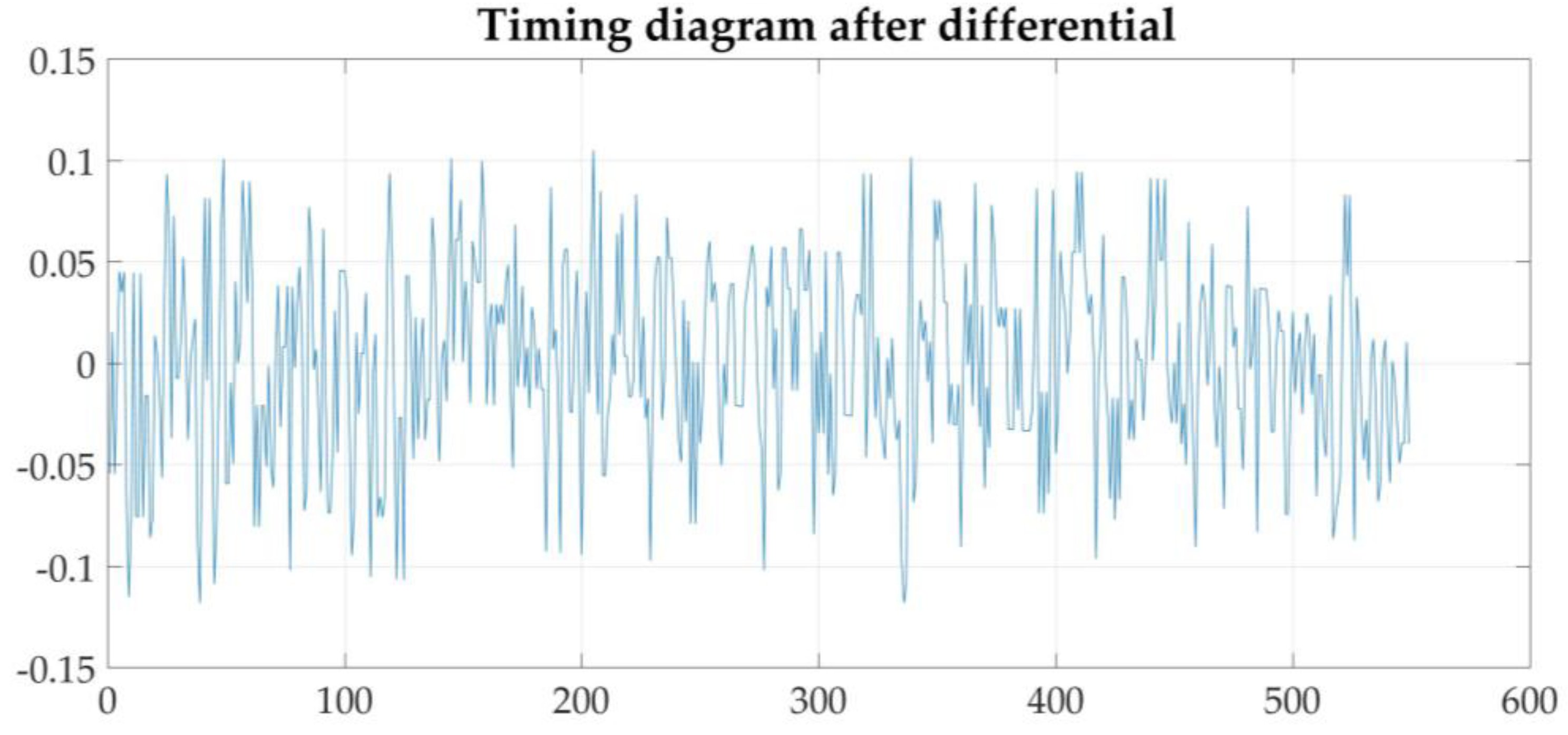
Figure 24.
Sequence diagram of dissolved oxygen after stability treatment.
Figure 24.
Sequence diagram of dissolved oxygen after stability treatment.
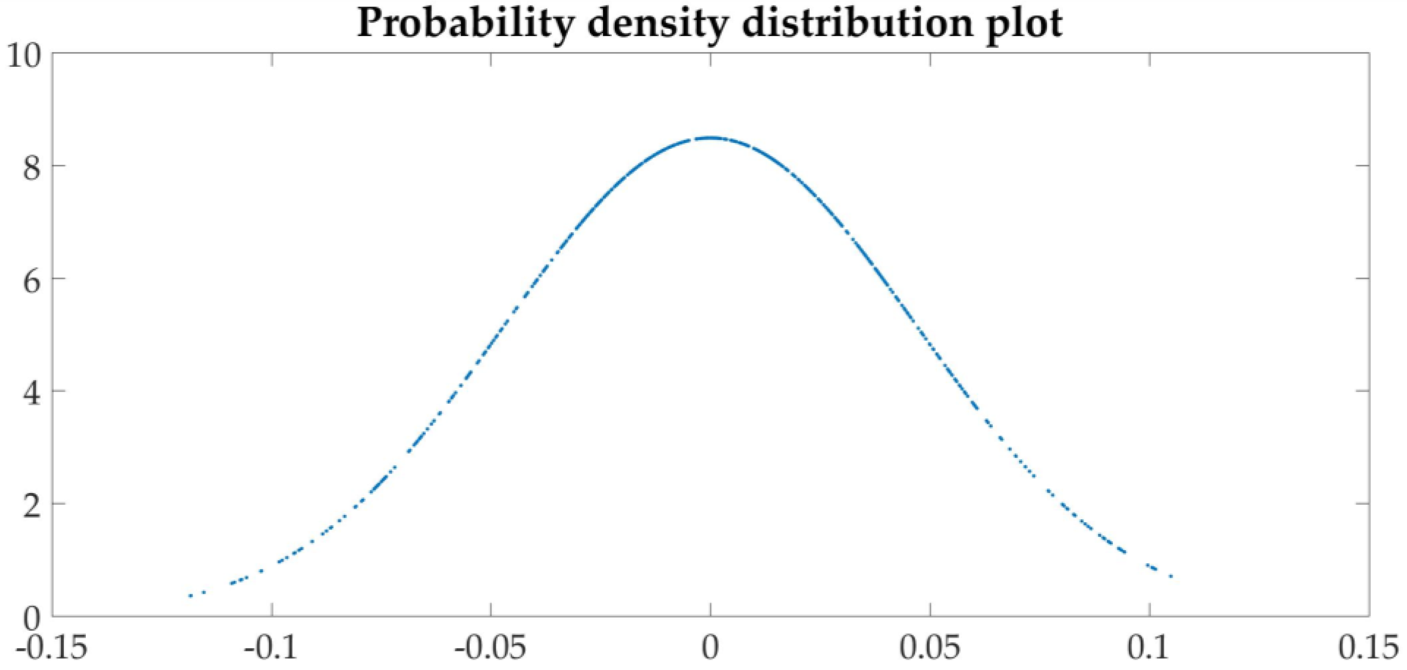
Figure 25.
Probability density distribution.
Figure 25.
Probability density distribution.
Figure 26.
Frequency distribution histogram.
Figure 26.
Frequency distribution histogram.
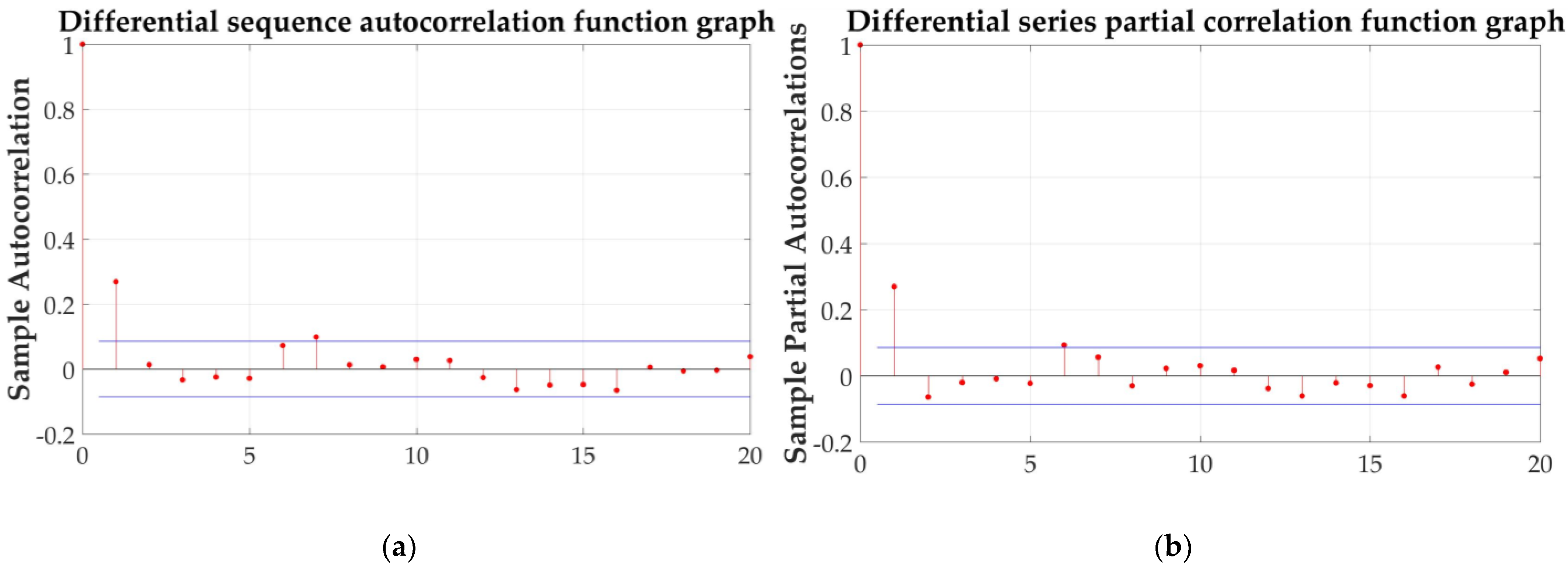
Figure 27.
(a) Autocorrelation function and (b) partial correlation function.
Figure 27.
(a) Autocorrelation function and (b) partial correlation function.
Figure 28.
Time series diagram of the fitted residual sequence.
Figure 28.
Time series diagram of the fitted residual sequence.
Figure 29.
Five steps: (a) probability density distribution; (b) frequency distribution histogram; (c) autocorrelation function; (d) partial correlation function; and (e) fitted residual sequence.
Figure 29.
Five steps: (a) probability density distribution; (b) frequency distribution histogram; (c) autocorrelation function; (d) partial correlation function; and (e) fitted residual sequence.
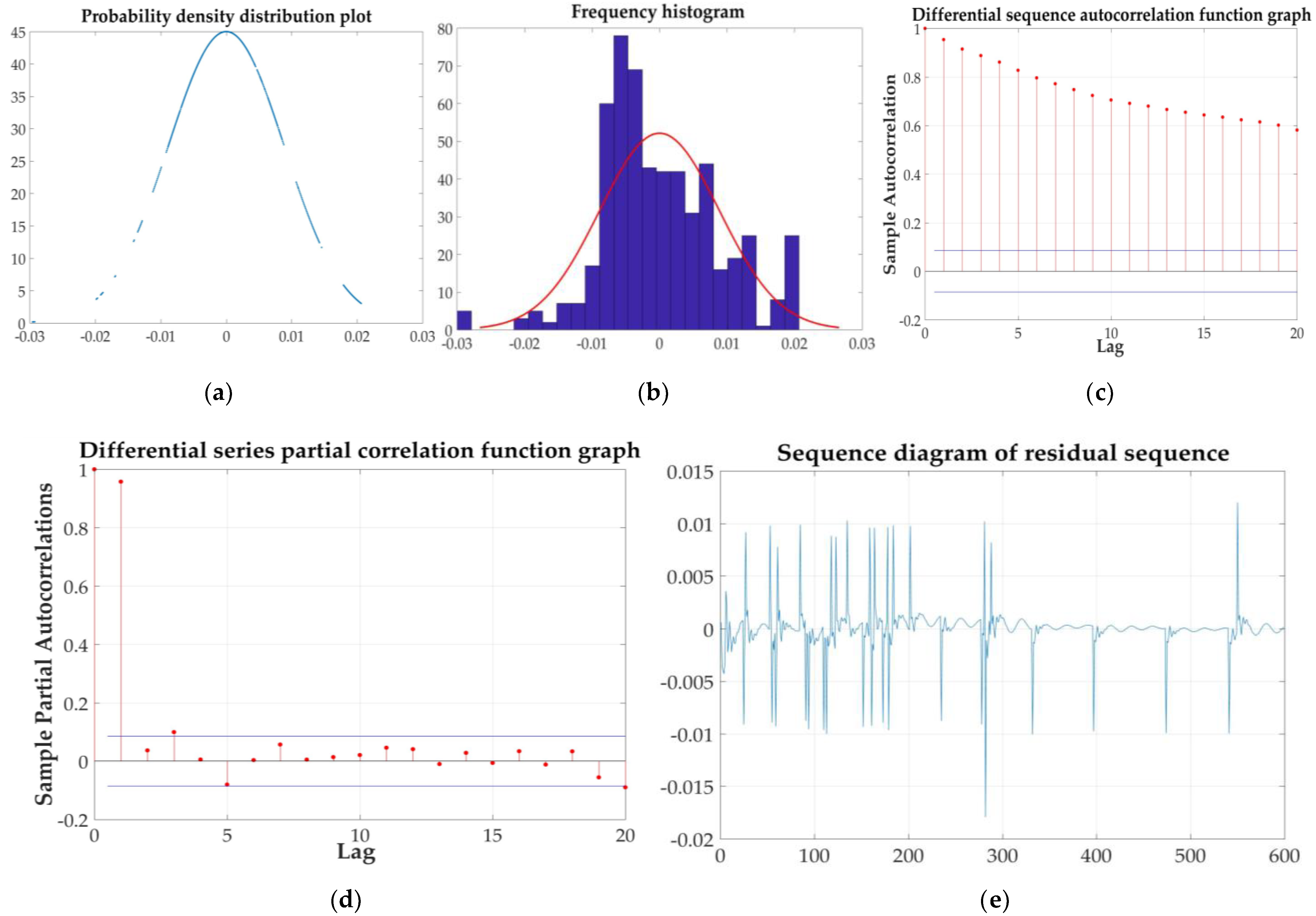
Figure 30.
Five steps: (a) probability density distribution; (b) frequency distribution histogram; (c) autocorrelation function; (d) partial correlation function; and (e) fitted residual sequence.
Figure 30.
Five steps: (a) probability density distribution; (b) frequency distribution histogram; (c) autocorrelation function; (d) partial correlation function; and (e) fitted residual sequence.
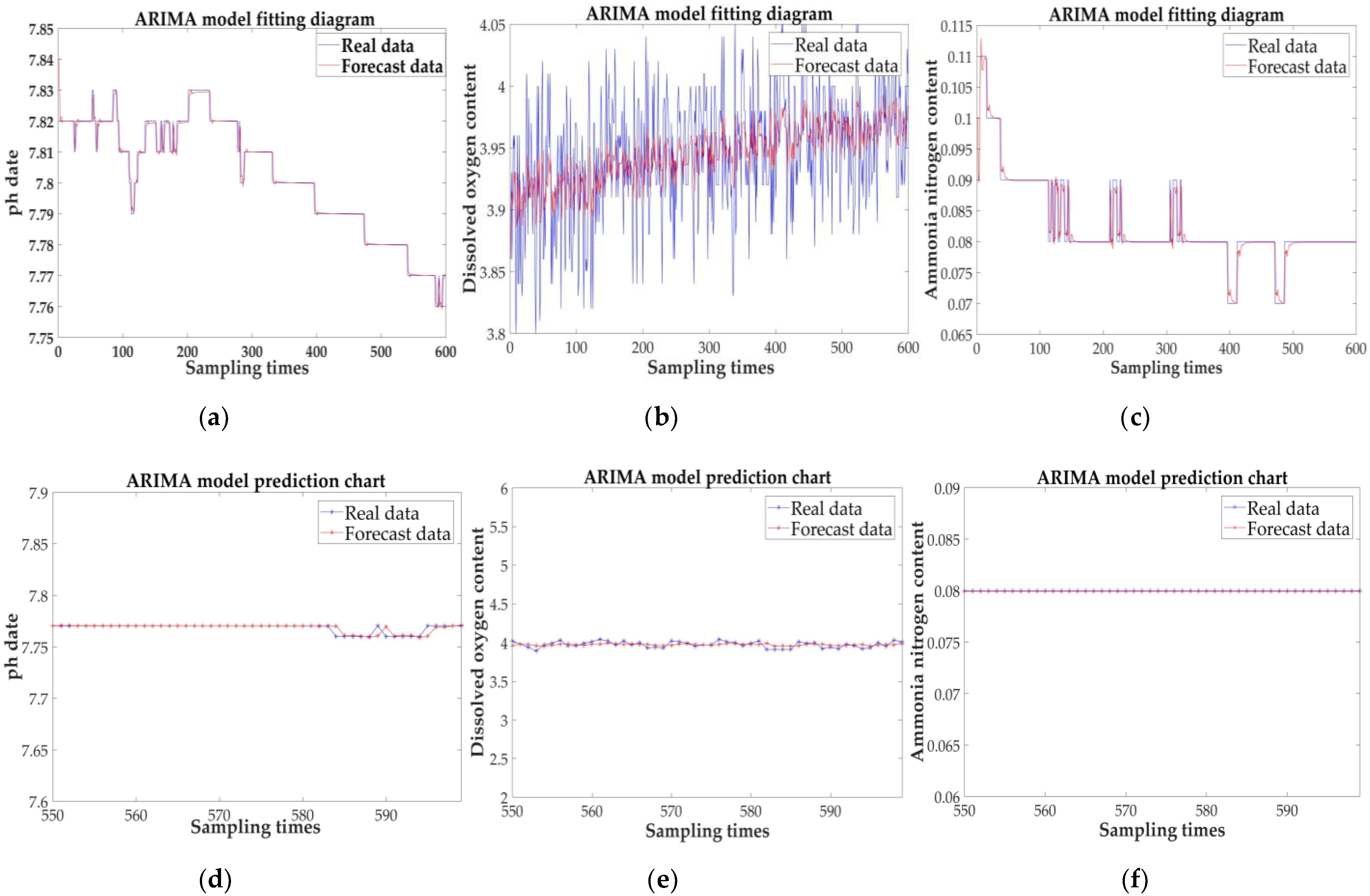
Figure 31.
Fitting graph and prediction graph of the three parameters: (a) fitting effect diagram under the pH; (b) fitting effect diagram under the DO; (c) fitting effect diagram under the ; (d) predicted results for pH; (e) predicted results for DO; and (f) predicted results for .
Figure 31.
Fitting graph and prediction graph of the three parameters: (a) fitting effect diagram under the pH; (b) fitting effect diagram under the DO; (c) fitting effect diagram under the ; (d) predicted results for pH; (e) predicted results for DO; and (f) predicted results for .
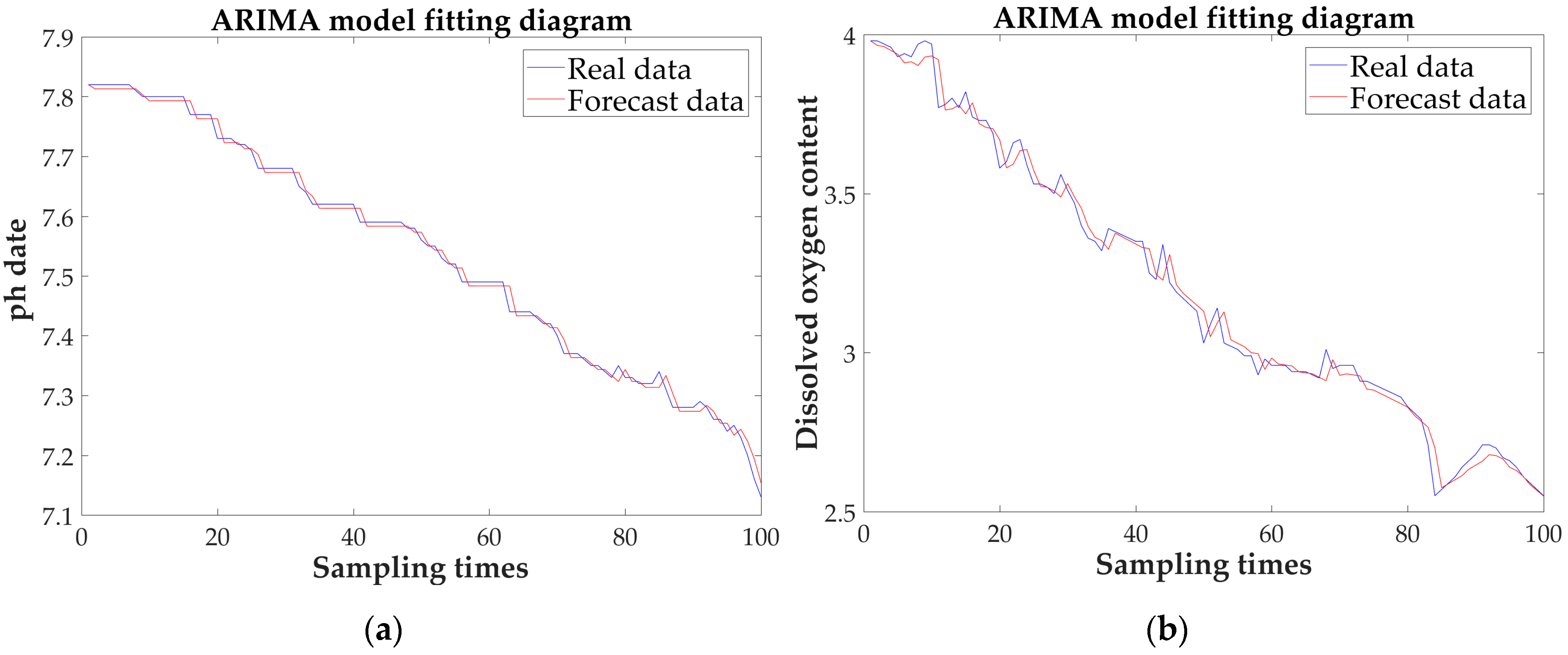
Figure 32.
Fitting graph and prediction graph of the three parameters: (a) fitting effect diagram under the pH; (b) fitting effect diagram under the DO; (c) fitting effect diagram under the ; (d) predicted results for pH; (e) predicted results for DO; and (f) predicted results for .
Figure 32.
Fitting graph and prediction graph of the three parameters: (a) fitting effect diagram under the pH; (b) fitting effect diagram under the DO; (c) fitting effect diagram under the ; (d) predicted results for pH; (e) predicted results for DO; and (f) predicted results for .
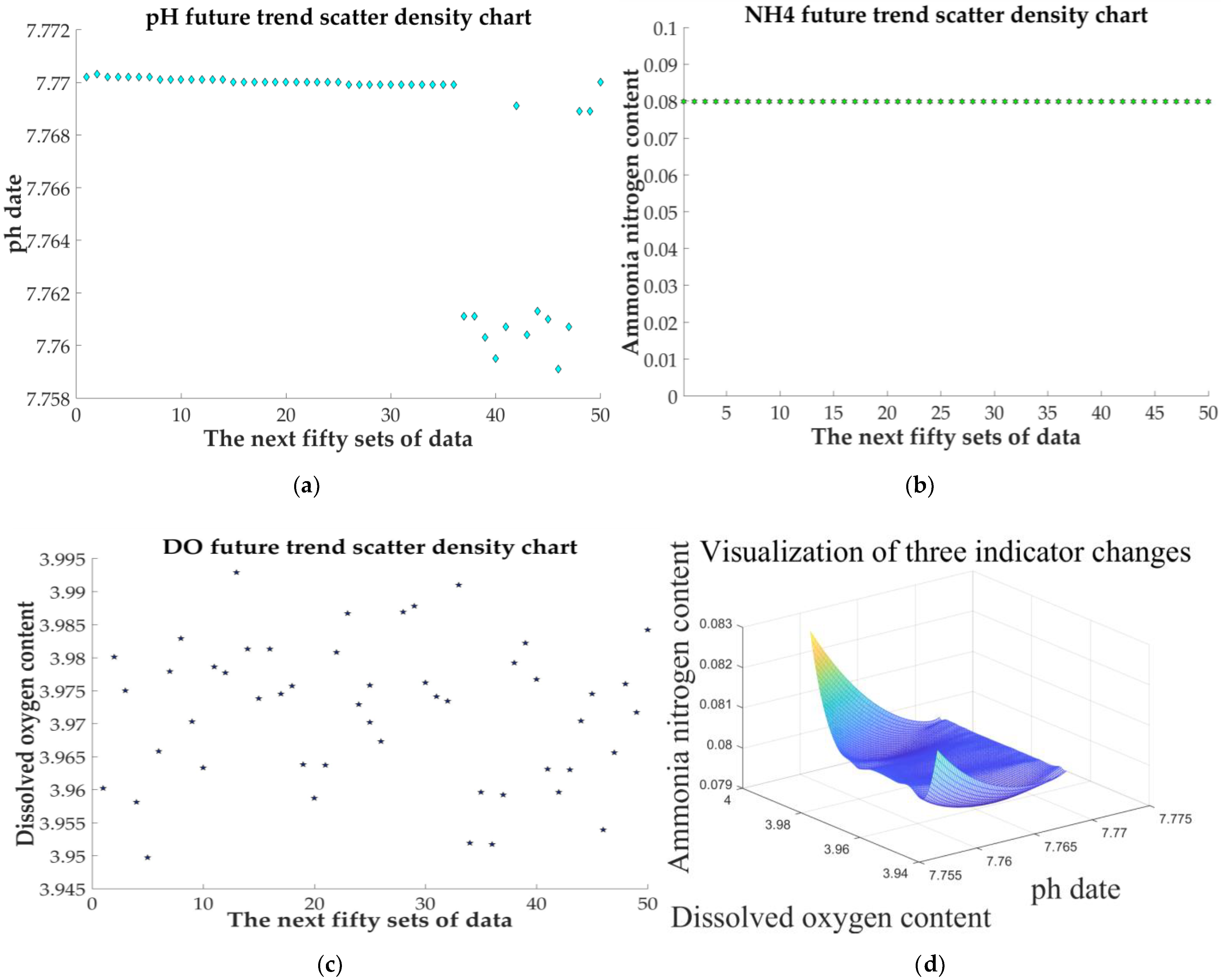
Figure 33.
The scatter plots and the overall visualization of the three sets of data changes: (a) pH; (b) ; (c) DO; and (d) visualization of three indicator changes.
Figure 33.
The scatter plots and the overall visualization of the three sets of data changes: (a) pH; (b) ; (c) DO; and (d) visualization of three indicator changes.
Figure 34.
Actual value of water quality monitoring at a certain moment.
Figure 34.
Actual value of water quality monitoring at a certain moment.
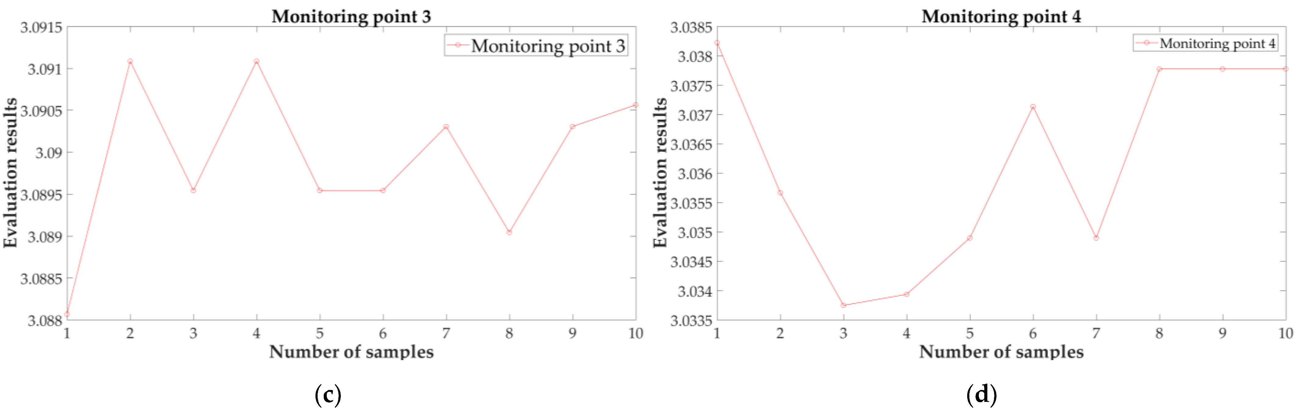
Figure 35.
The water quality in different regions: (a) monitoring point 1; (b) monitoring point 2; (c) monitoring point 3; and (d) monitoring point 4.
Figure 35.
The water quality in different regions: (a) monitoring point 1; (b) monitoring point 2; (c) monitoring point 3; and (d) monitoring point 4.
Table 1.
Water quality prediction methods.
Table 1.
Water quality prediction methods.
| Classification | Use | Limitation |
|---|
| Nonmechanical methods | Gray model prediction [16,17,18] | Make medium and long-term forecasts | Large deviation |
| Time series analysis [19,20,21,22] | Random time series method | Markov | Manage data that are difficult to express as a function of time | Large amount of data support |
| Box–Jenkins |
| Deterministic time series | Time series smoothing | The original data changes have a certain law | Cannot handle data that are difficult to express as a function of time |
| Trend extrapolation |
| Seasonal variation forecast |
| Artificial neural network prediction [23,24,25] | Long Short-Term Memory (deep learning method) | Improve unstable time series with more fixed components. | High requirements for development time, data volume, and calculation cost |
| Back Propagation neural network | Nonlinear time series data |
| Mechanism methods | Water quality numerical model [26,27,28] | Need extensive hydrological data modeling |
Table 2.
Water quality evaluation method.
Table 2.
Water quality evaluation method.
| Classification Method | Evaluation Method |
|---|
| Stage | Review evaluation |
| Present situation evaluation |
| Prejudge evaluation |
| Use | Agricultural irrigation |
| Industrial production |
| Domestic drinking |
| Index number relationship | Single-factor evaluation |
| Multi-factor evaluation |
| Type of water body | Surface water quality evaluation |
| Groundwater quality evaluation |
| Method | Fuzzy comprehensive evaluation method [29,30,31] |
| Artificial neural network evaluation method |
Table 3.
Parameters of three electrode probes.
Table 3.
Parameters of three electrode probes.
| Parameter Index | pH Probe | Dissolved Oxygen Probe | Ammonia Nitrogen Probe |
|---|
| Measuring range | 0–14 pH | 0–20 mg/L | 0–10 mg/L |
| Resolution | 0.01 pH, 0.1 °C | 0.01 mg/L, 0.1 °C | 0.01 mg/L, 0.1 °C |
| Precision | ±0.02 pH, ±0.2 °C | ±0.5% FS, ±0.3 °C | ±1% FS, ±0.3 °C |
| Output load | <300 Ω | <300 Ω | <300 Ω |
| Working voltage | DC12V | DC12V | DC12V |
Table 4.
Fishery water index ranges corresponding to the three index factors studied in this paper.
Table 4.
Fishery water index ranges corresponding to the three index factors studied in this paper.
| Index Factor | Index Range |
|---|
| pH | 6.5–8.5 (freshwater) |
| DO | ≥3 mg/L |
| NH4 ± N | ≤2 mg/L |
Table 5.
Surface Water Environmental Quality Standard GB3828-2002.
Table 5.
Surface Water Environmental Quality Standard GB3828-2002.
| Index Factor | Class I | Class II | Class III | Class IV | Class V |
|---|
| pH | 7.0–8.0 | 6.0–7.0/8.0–9.0 | 5.0–6.0/9.0–10.0 | 4.0–5.0/10.0–11.0 | 0–4/11–14 |
| DO | 8 | 6–8 | 4–6 | 2–4 | 0–2 |
| 0–0.2 | 0.2–0.5 | 0.5–1.0 | 1.0–1.5 | 2.0 |
Table 6.
Water quantitative evaluation index.
Table 6.
Water quantitative evaluation index.
| Quantify Grade/Range/Score | pH | DO | | Network Output Range (3.0–3.3) |
|---|
| Excellent/(90–100)/100 | 6–8 | 4–8 | ≤0.2 | 3.0–3.1 |
| Good/(70–90)/70 | 5–6 or 8–9 | 2–4 or 8–10 | 0.2–0.3 | 3.1–3.2 |
| Poor/(<70)/40 | <5 or >9 | <2 or >10 | >0.3 | 3.2–3.3 |
| Weight | 0.4 | 0.3 | 0.3 | |
Table 7.
The monitoring results of two sets of water quality sensors connected to the IoT platform.
Table 7.
The monitoring results of two sets of water quality sensors connected to the IoT platform.
| | Water Quality Monitoring Experiment | Water Quality Monitoring Comparison Experiment |
|---|
| pH | 6.68 pH | 6.68 pH |
| Dissolved oxygen | 4.75 mg/L | 4.45 mg/L |
| Ammonia nitrogen content | 0.15 mg/L | 0.14 mg/L |
| Temperature | 12.5 °C | 12.4 °C |
Table 8.
Monitoring flight process indicators.
Table 8.
Monitoring flight process indicators.
| Index | Value | Index | Value | Index | Value |
|---|
| Number of monitoring points | 4 | The distance between monitoring points 1 and 2 | 102 m | Monitoring region area | 200,000 m2 |
| Number of takeoffs | 4 | The distance between monitoring points 2 and 3 | 208 m | Task execution time | 157 min |
| Number of landings | 4 | The distance between monitoring points 3 and 4 | 70 m | Starting point voltage | 25.25 V |
| Total number of takeoffs and landings | 5 | Total horizontal route | 760 m | End point voltage | 22.60 V |
Table 9.
Analysis of the maximum error in the prediction results of pH value, dissolved oxygen content, and ammonia nitrogen content in the sunny experiment.
Table 9.
Analysis of the maximum error in the prediction results of pH value, dissolved oxygen content, and ammonia nitrogen content in the sunny experiment.
| Sequence | Real Data | Predicted Data | Absolute Error | Relative Error |
|---|
| pH | 7.77 | 7.7595 | 0.0105 | 0.135% |
| DO | 3.89 | 3.9581 | −0.0681 | 1.751% |
| NH4 ± N | 0.08 | 0.079875 | 0.000125 | 0.156% |
Table 10.
Analysis of the maximum error in the prediction results of pH value, dissolved oxygen content, and ammonia nitrogen content in the rainy experiment.
Table 10.
Analysis of the maximum error in the prediction results of pH value, dissolved oxygen content, and ammonia nitrogen content in the rainy experiment.
| Sequence | Real Data | Predicted Data | Absolute Error | Relative Error |
|---|
| pH | 7.77 | 7.16 | 0.61 | 7.851% |
| DO | 2.71 | 2.659 | 0.051 | 1.882% |
| NH4 ± N | 0.1 | 0.1092 | −0.0092 | 9.2% |


