
Numerical Analysis of 2-D Positioned, Indoor, Fuzzy-Logic, Autonomous Navigation System Based on Chromaticity and Frequency-Component Analysis of LED Light


Abstract
:1. Introduction
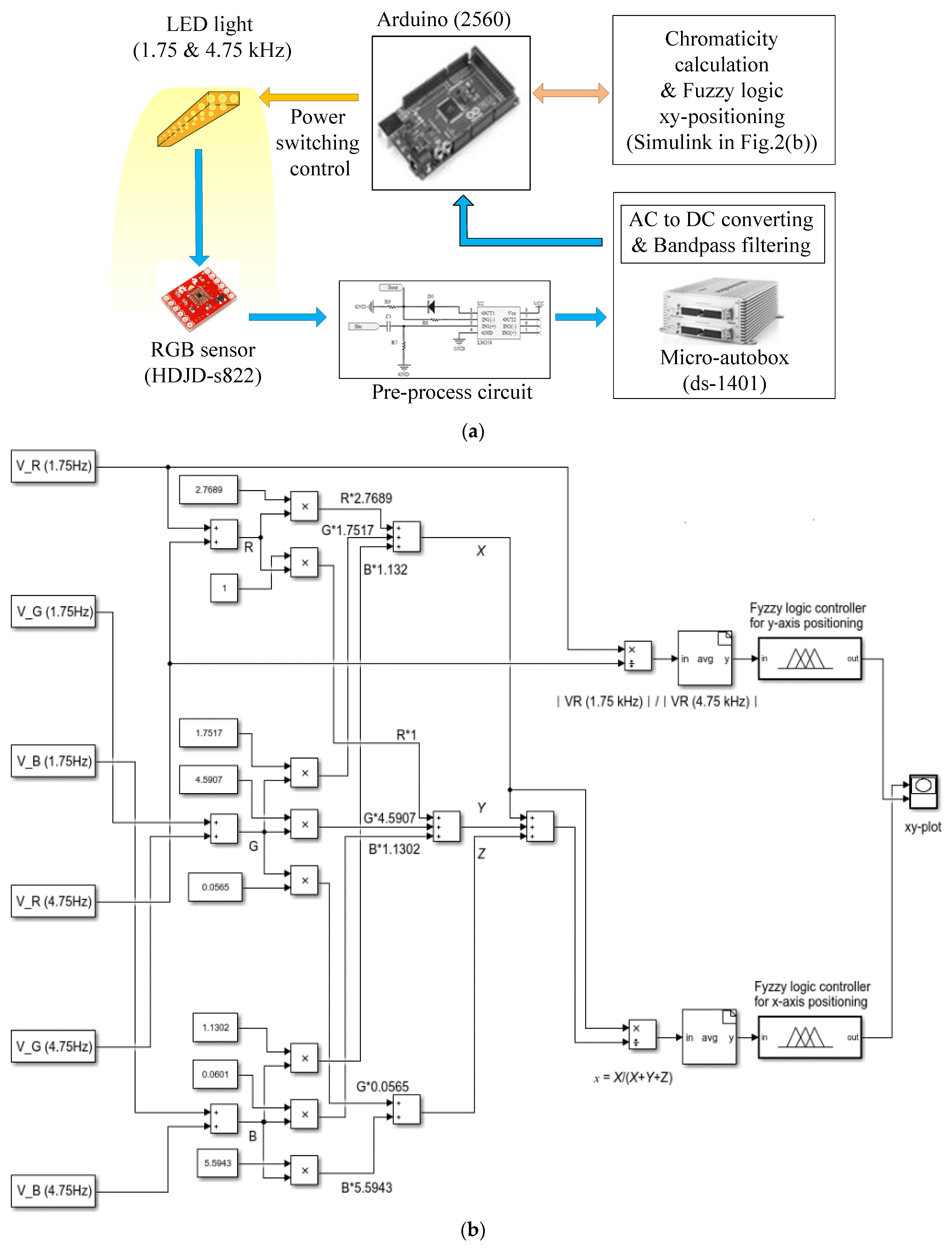
2. Positioning Method
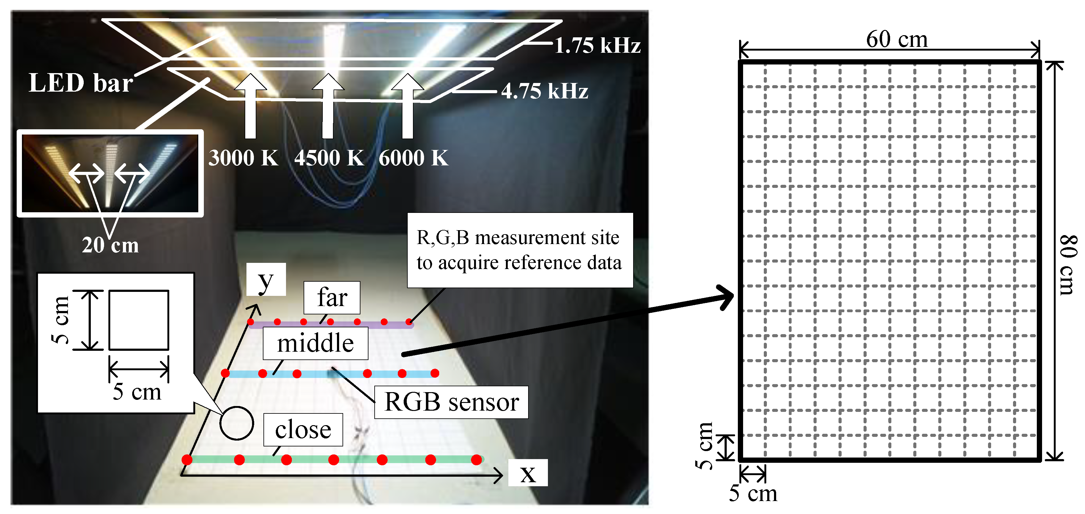
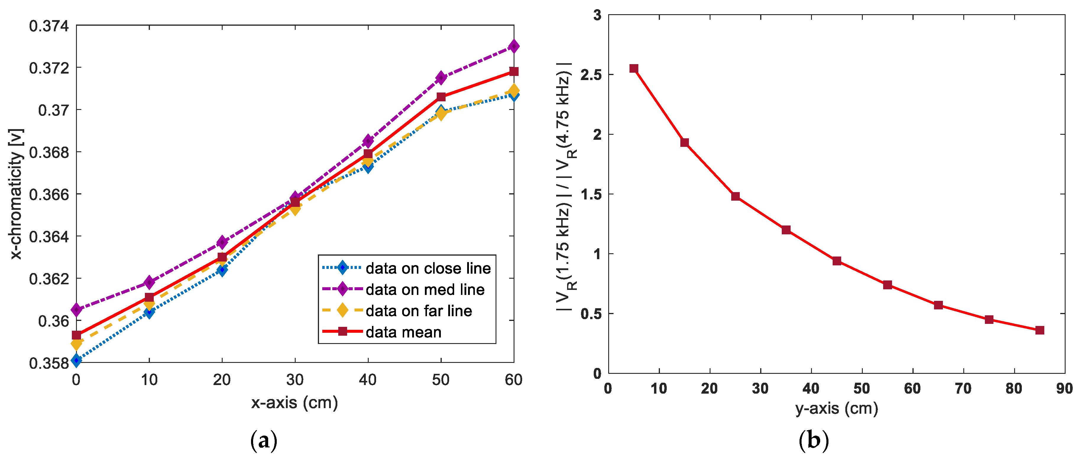
2.1. Experimental Environment
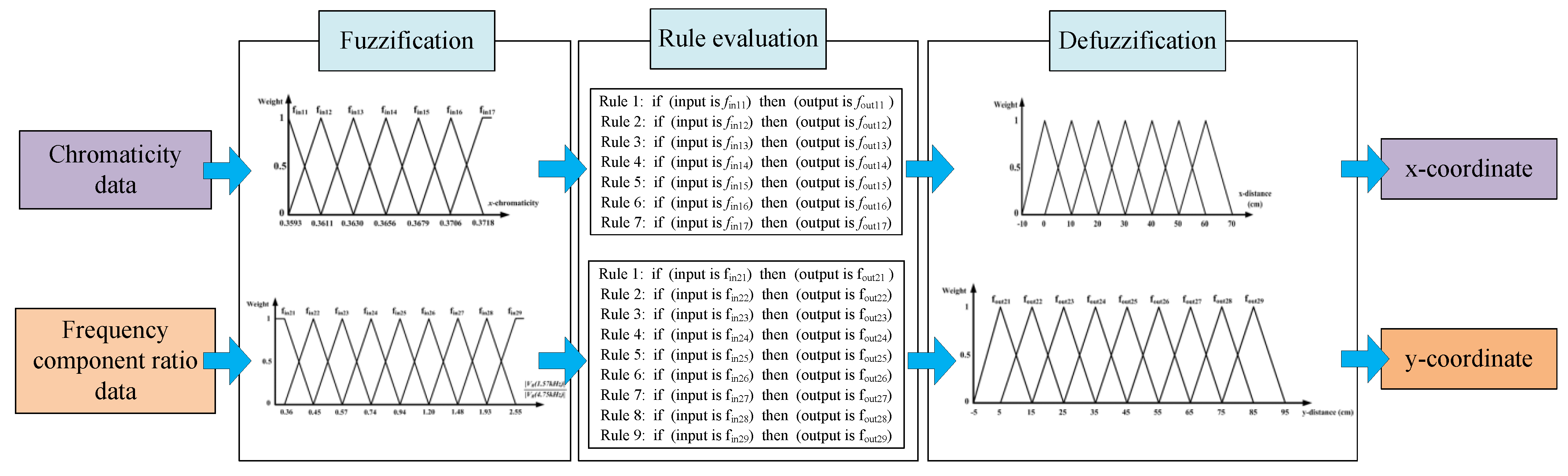
2.2. Fuzzy Positioning System
3. Fuzzy-Logic Autonomous Navigation System
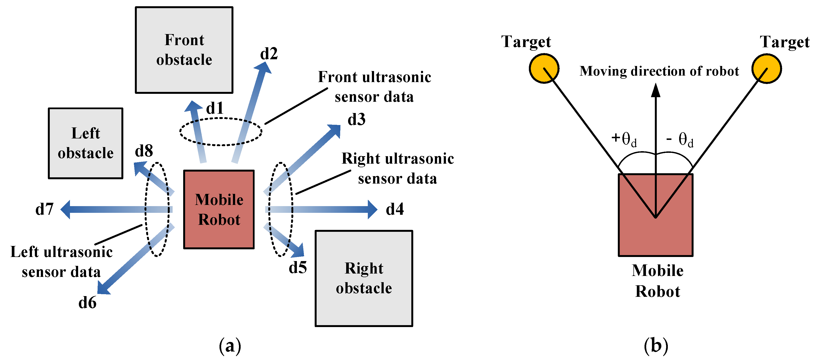
3.1. Sensors of Navigation System
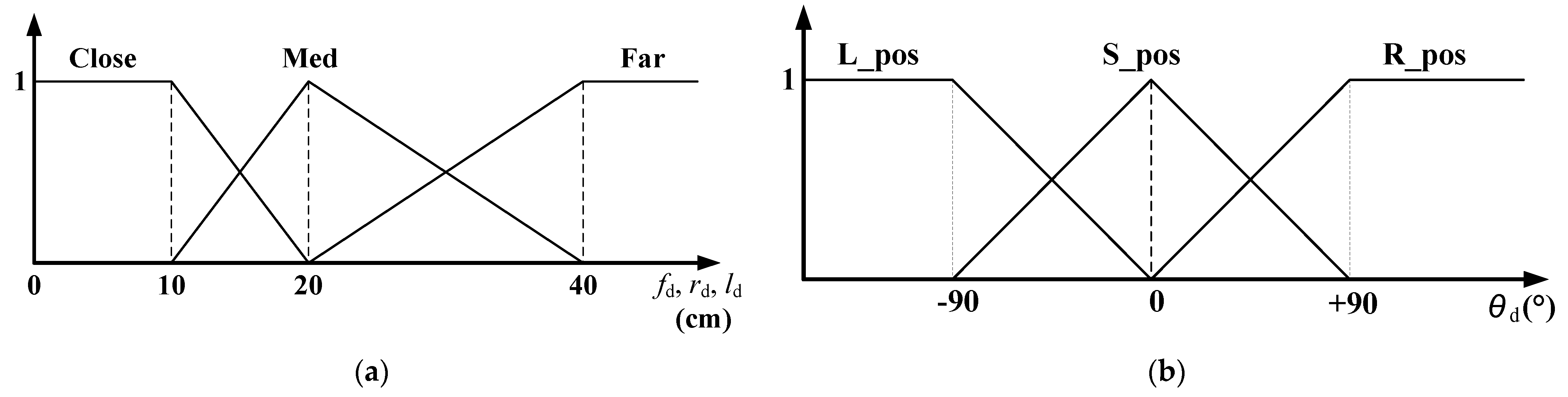
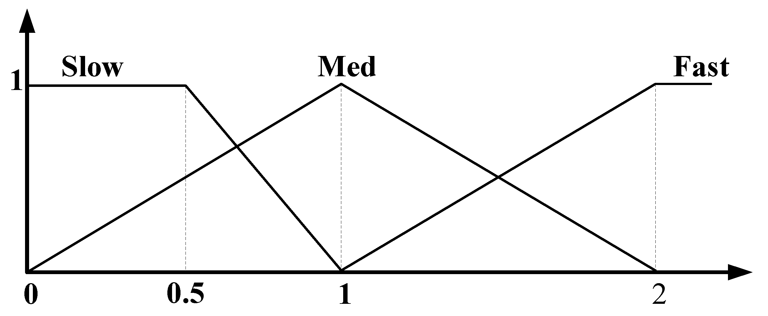
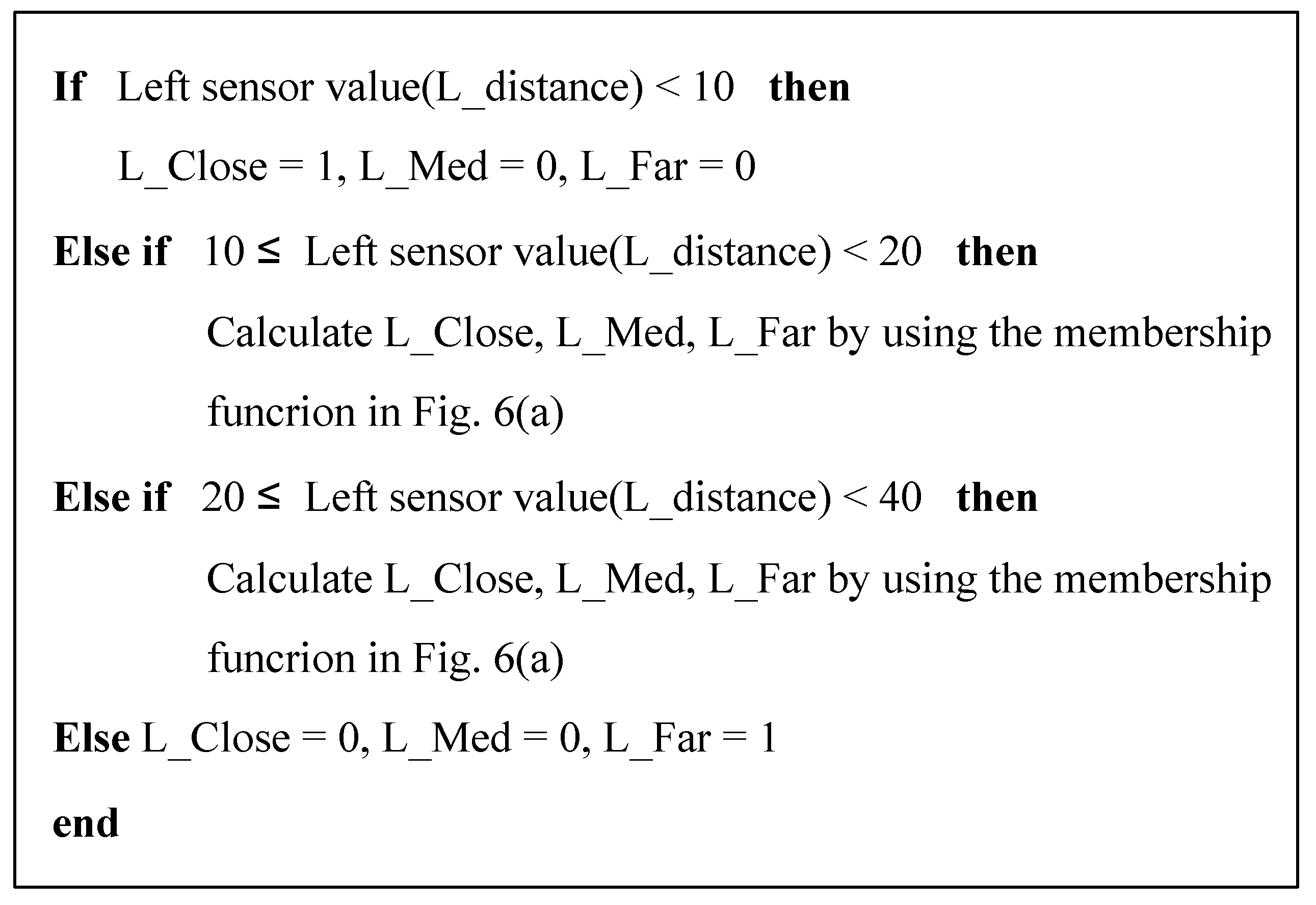
3.2. Fuzzification Process of Distance Data
3.3. Behavior Rule-Evaluation Process
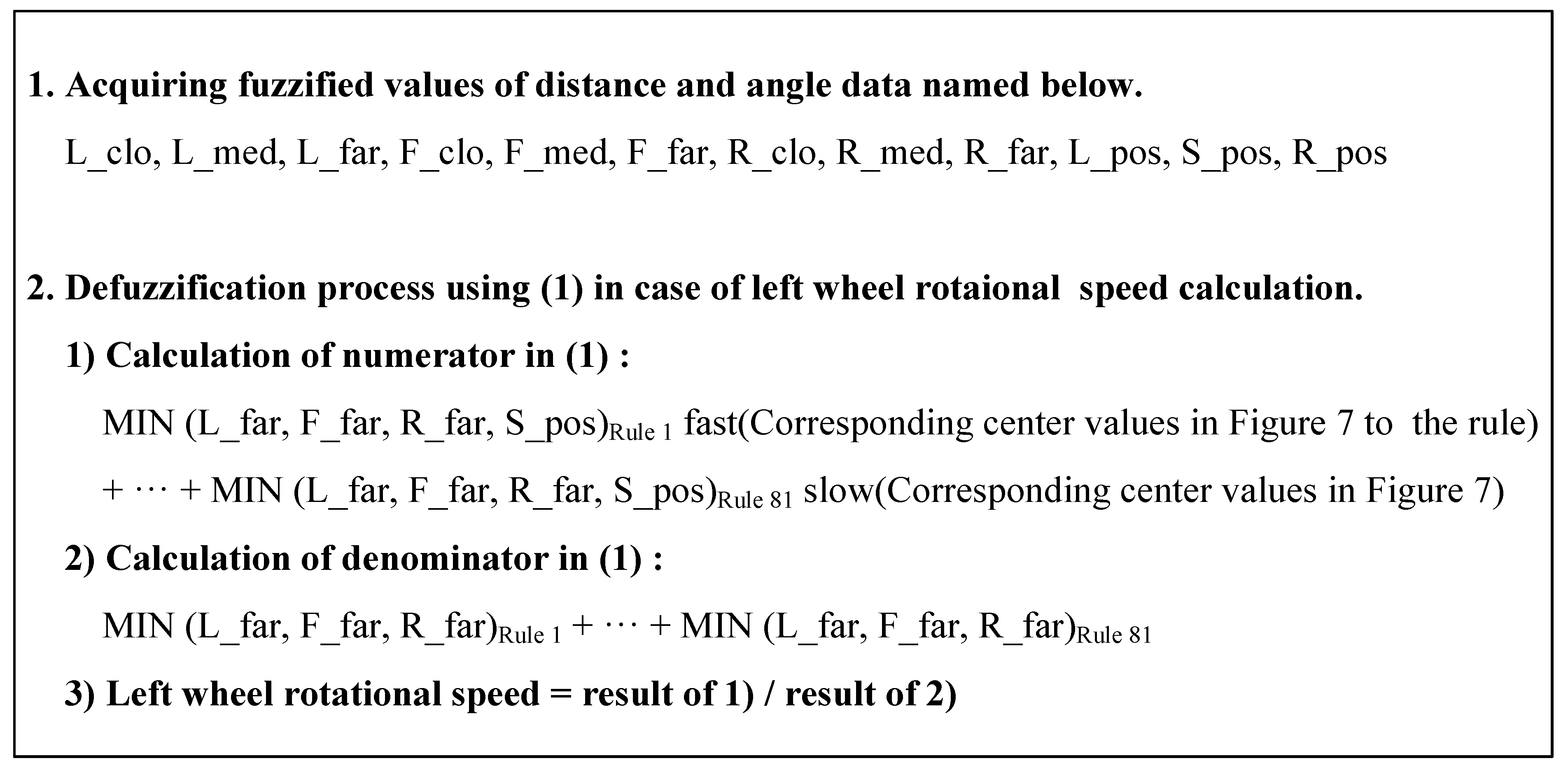
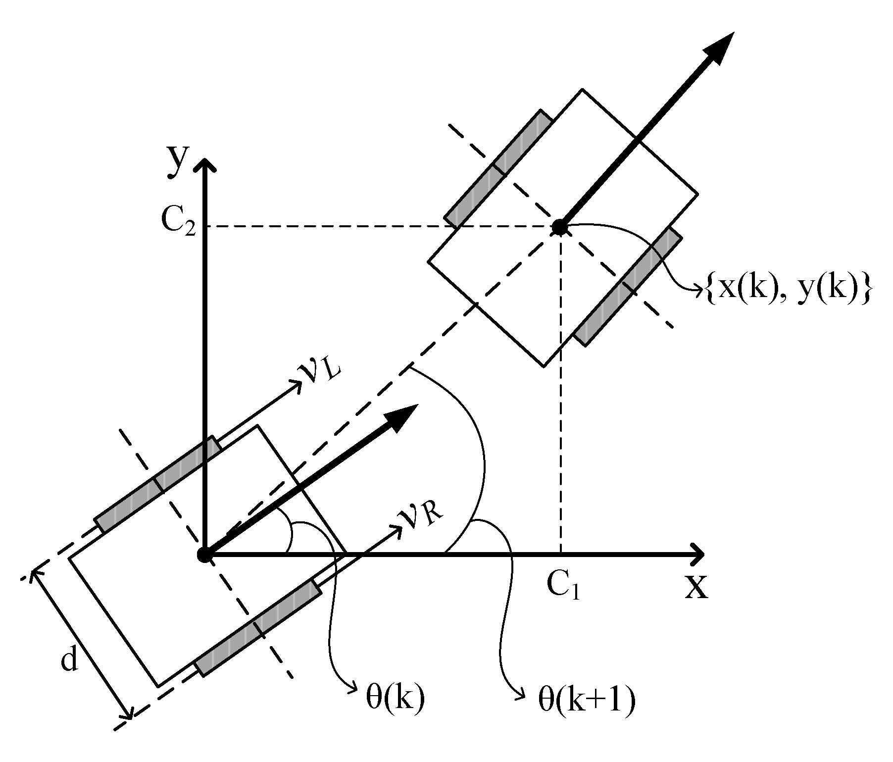
3.4. Defuzzification Process to Produce Robot Motion
4. Potential Field Autonomous Navigation System
4.1. Sensors of the Navigation System
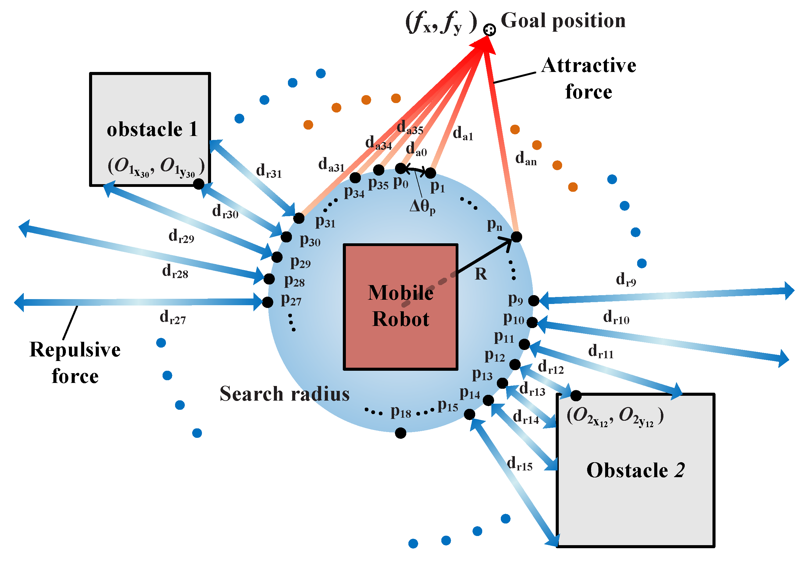
4.2. Potential Field Navigation Algorithm
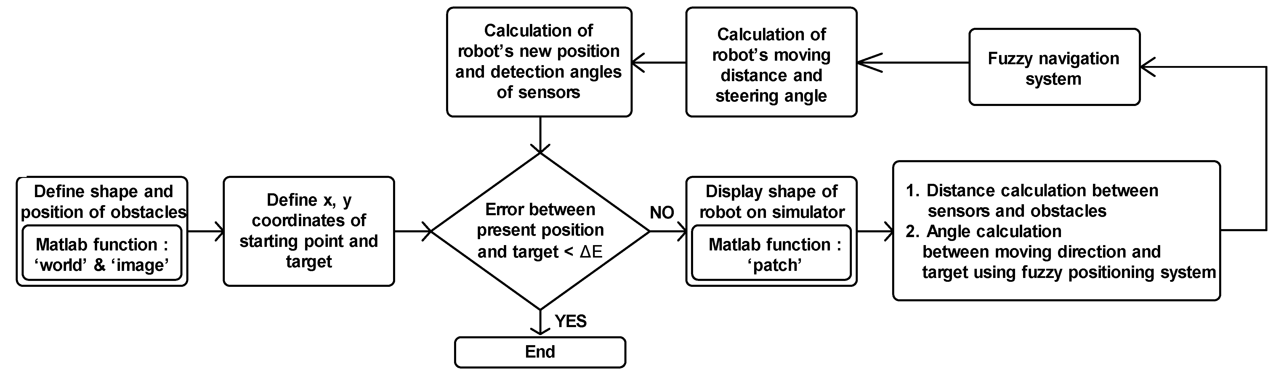
5. Design of Autonomous Navigation Simulator
6. Results
7. Conclusions
Author Contributions
Funding
Institutional Review Board Statement
Informed Consent Statement
Acknowledgments
Conflicts of Interest
References
- Jeong, J.H.; Lee, D.H.; Byun, G.S.; Cho, H.R.; Cho, Y.H. The tunnel lane positioning system of an autonomous vehicle in the LED lighting. J. Korean Inst. Intell. Transp. Syst. 2017, 16, 186–195. [Google Scholar] [CrossRef]
- Jeong, J.H.; Kim, M.; Byun, G.S. Position recognition for an autonomous vehicle based on vehicle-to-led infrastructure. AETA 2016 Recent Adv. Electr. Eng. Relat. Sci. Lect. Notes Electr. Eng. 2017, 415, 913–921. [Google Scholar]
- Kong, S.H.; Jeong, G.S. GPS/GNSS based vehicular positioning and navigation techniques. Int. J. Automot. Technol. 2015, 37, 24–28. [Google Scholar]
- Kong, S.H.; Jeon, S.Y.; Ko, H.W. Status and trends in the sensor fusion positioning technology. J. Korean Inst. Commun. Inf. Sci. 2015, 32, 45–53. [Google Scholar]
- Lee, J.K. Automatic driving cars developments trends and implications. Inst. Korean Electr. Electron. Eng. 2015, 64, 24–28. [Google Scholar]
- Kabanza, F.; Lamine, K.B. Specifying failure and progress conditions in a behavior-based robot programming system. In Proceedings of the 4th International Cognitive Robotics Workshop, Valencia, Spain, 23−24 August 2004; pp. 11–16. [Google Scholar]
- Li, W. Fuzzy Logic-Based ‘Perception-action’ behavior control of mobile robot in uncertain environments. Proc. IEEE Int. Conf. Fuzzy Syst. 1994, 3, 1626–1631. [Google Scholar]
- Zhang, N.; Beetner, D.; Wunsch, D.C., II; Hemmelman, B.; Hasan, A. An embedded real-time neuro-fuzzy controller for mobile robot navigation. In Proceedings of the 14th IEEE International Conference on Fuzzy Systems, 2005. FUZZ ‘05, Reno, NV, USA, 25 May 2005; pp. 319–323. [Google Scholar]
- Pandey, A.; Pandey, S.; DR, P. Mobile robot navigation and obstacle avoidance technique: A review. Int. J. Robot. Autom. 2017, 2, 96–105. [Google Scholar] [CrossRef] [Green Version]
- Yun, D.S.; Yu, H.S. Development of the optimized autonomous navigation algorithm for the unmanned vehicle using extended Kalman filter. Korean Soc. Automot. Eng. 2008, 16, 7–14. [Google Scholar]
- Chung, B.M.; Seok, J.W.; Cho, C.S.; Lee, J.W. Autonomous tracking control of intelligent vehicle using GPS information. J. Korean Soc. Precis. Eng. 2008, 25, 58–66. [Google Scholar]
- Zhu, H.; Yuen, K.-V.; Mihaylova, L.; Leung, H. Overview of environment perception for intelligent vehicles. IEEE Trans. Intell. Transp. Syst. 2017, 18, 2584–2601. [Google Scholar] [CrossRef] [Green Version]
- Wang, J.; Schroedl, S.; Mezger, K.; Ortloff, R.; Joos, A.; Passegger, T. Lane keeping based on location technology. IEEE Trans. Intell. Transp. Syst. 2005, 6, 351–356. [Google Scholar] [CrossRef]
- Ma, B.; Lakshmanan, S.; Hero, A.O. Simultaneous detection of lane and pavement boundaries using model-based multisensor fusion. IEEE Trans. Intell. Transp. Syst. 2000, 1, 135–147. [Google Scholar] [CrossRef]
- Topfer, D.; Spehr, J.; Effertz, J.; Stiller, C. Efficient road scene understanding for intelligent vehicles using compositional hierarchical models. IEEE Trans. Intell. Transp. Syst. 2015, 16, 441–451. [Google Scholar] [CrossRef]
- Nakajima, M.; Haruyama, S. New indoor navigation system for visually impaired people using visible light communication. EURASIP J. Wirel. Commun. Netw. 2013, 2013, 37–46. [Google Scholar] [CrossRef] [Green Version]
- Vongkulbhisal, J.; Chantaramolee, B.; Zhao, Y.; Mohammed, W.S. A fingerprinting-based indoor localization system using intensity modulation of light emitting diodes. Microw. Opt. Technol. Lett. 2012, 54, 1218–1227. [Google Scholar] [CrossRef]
- Kim, H.S.; Kim, D.R.; Yang, S.H.; Son, Y.H.; Han, S.K. An indoor visible light communication positioning system using a RF carrier allocation technique. J. Lightwave Technol. 2012, 31, 134–144. [Google Scholar] [CrossRef]
- Cossu, G.; Presi, M.; Corsini, R.; Choudhury, P.; Khalid, A.M.; Ciaramella, E. A visible light localization aided optical wireless system. In Proceedings of the IEEE GLOBECOM Workshops, Houston, TX, USA, 5–9 December 2011; pp. 802–807. [Google Scholar]
- Zhuang, Y.; Hua, L.; Qi, L.; Yang, J.; Cao, P.; Cao, Y.; Wu, Y.; Thompson, J.; Haas, H. A survey of positioning systems using visible LED lights. IEEE Commun. Surv. Tutor. 2018, 20, 1963–1988. [Google Scholar] [CrossRef] [Green Version]
- del Campo-Jimenez, G.; Perandones, J.M.; Lopez-Hernandez, F.J. A VLC-based beacon location system for mobile applications. In Proceedings of the IEEE International Conference on Localization and GNSS (ICL-GNSS), Turin, Italy, 25–27 June 2013; pp. 1–4. [Google Scholar]
- Fang, J.; Yang, Z.; Long, S.; Wu, Z.; Zhao, X.; Liang, F.; Jiang, Z.L.; Chen, Z. High-speed indoor navigation system based on visible light and mobile phone. IEEE Photonics J. 2017, 9, 1–11. [Google Scholar] [CrossRef]
- Rahman, M.S.; Haque, M.M.; Kim, K.-D. Indoor positioning by LED visible light communication and image sensors. Int. J. Electr. Comput. Eng. 2011, 1, 161–170. [Google Scholar] [CrossRef]
- Jeong, J.H.; Byun, G.S.; Park, K. Fuzzy logic vehicle positioning system based on chromaticity and frequency components of LED illumination. IEEE Photonics J. 2019, 11, 1–12. [Google Scholar] [CrossRef]
- Ünal, A.S.İ.L.; Erkan, U.S.L.U. Potential field path planning and potential field path tracking. In Proceedings of the Innovations in Intelligent Systems and Applications Conference (ASYU), Istanbul, Turkey, 15–17 October 2020; pp. 1–4. [Google Scholar]
- Lin, X.; Wang, Z.-Q.; Chen, X.-Y. Path planning with improved artificial potential field method based on decision tree. In Proceedings of the 27th Saint Petersburg International Conference on Integrated Navigation Systems (ICINS), Saint Petersburg, Russia, 25–27 May 2020; pp. 1–5. [Google Scholar]


| Rule | if | ld | and | fd | and | rd | and | θd | then | LVel | and | RVel |
|---|---|---|---|---|---|---|---|---|---|---|---|---|
| 1 | if | Far | and | Far | and | Far | and | S_pos | then | Fast | and | Fast |
| 2 | Far | Far | Far | L_pos | Fast | Slow | ||||||
| 3 | Far | Far | Far | R_pos | Slow | Fast |
| Rule | if | ld | and | fd | and | rd | and | θd | then | LVel | and | RVel |
|---|---|---|---|---|---|---|---|---|---|---|---|---|
| 4 | if | Far | and | Far | and | Close | and | L_pos | then | Med | and | Med |
| 5 | Close | Far | Far | R_pos | Med | Med |
| Rule | if | ld | and | fd | and | rd | and | θd | then | LVel | and | RVel |
|---|---|---|---|---|---|---|---|---|---|---|---|---|
| 6 | if | Med | and | Close | and | Close | and | any | then | Slow | and | Fast |
| 7 | Close | Close | Med | any | Fast | Slow | ||||||
| 8 | Close | Med | Close | any | Med | Med |
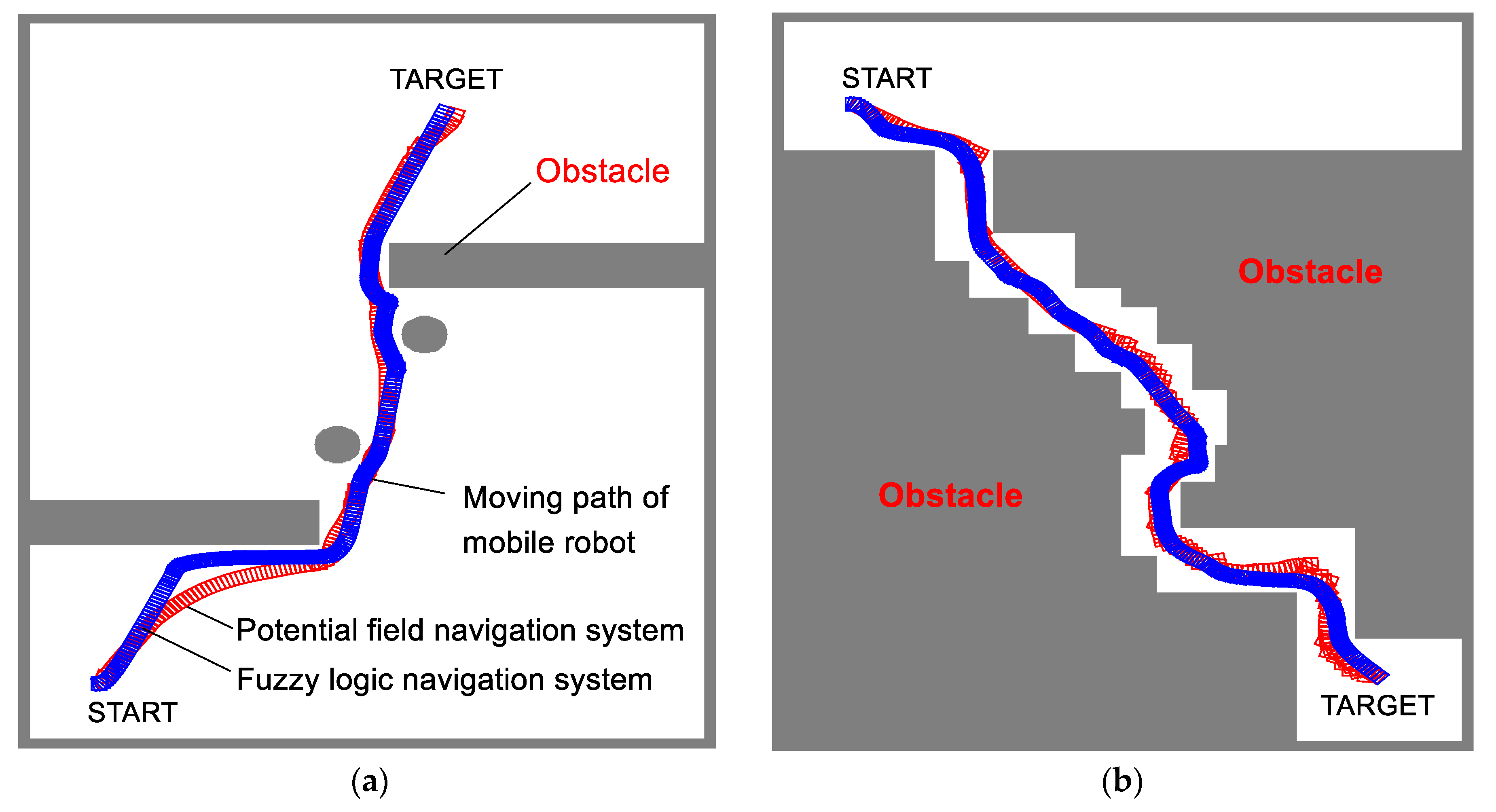
| Simulation Data | Simulation 1 (Figure 13a) | Simulation 2 (Figure 13b) | Simulation 3 (Figure 13c) | Simulation 4 (Figure 13d) | |
|---|---|---|---|---|---|
| Length of path | Fuzzy logic navigation | 79.60 cm | 88.41 cm | 111.86 cm | 299.78 cm |
| Potential field navigation | 77.36 cm | 105.11 cm | 128.90 cm | 333.40 cm | |
| Navigation time | Fuzzy logic navigation | 99.34 s | 133.33 s | 161.39 s | 312.21 s |
| Potential field navigation | 57.43 s | 76.24 s | 92.74 s | 223.10 s | |
| Mean of velocity | Fuzzy logic navigation | 0.80 cm/s | 0.66 cm/s | 0.69 cm/s | 0.96 cm/s |
| Potential field navigation | 1.35 cm/s | 1.38 cm/s | 1.39 cm/s | 1.49 cm/s | |
Publisher’s Note: MDPI stays neutral with regard to jurisdictional claims in published maps and institutional affiliations. |
© 2021 by the authors. Licensee MDPI, Basel, Switzerland. This article is an open access article distributed under the terms and conditions of the Creative Commons Attribution (CC BY) license (https://creativecommons.org/licenses/by/4.0/).
Share and Cite
Jeong, J.-H.; Park, K. Numerical Analysis of 2-D Positioned, Indoor, Fuzzy-Logic, Autonomous Navigation System Based on Chromaticity and Frequency-Component Analysis of LED Light. Sensors 2021, 21, 4345. https://doi.org/10.3390/s21134345
Jeong J-H, Park K. Numerical Analysis of 2-D Positioned, Indoor, Fuzzy-Logic, Autonomous Navigation System Based on Chromaticity and Frequency-Component Analysis of LED Light. Sensors. 2021; 21(13):4345. https://doi.org/10.3390/s21134345
Chicago/Turabian StyleJeong, Jae-Hoon, and Kiwon Park. 2021. "Numerical Analysis of 2-D Positioned, Indoor, Fuzzy-Logic, Autonomous Navigation System Based on Chromaticity and Frequency-Component Analysis of LED Light" Sensors 21, no. 13: 4345. https://doi.org/10.3390/s21134345
APA StyleJeong, J.-H., & Park, K. (2021). Numerical Analysis of 2-D Positioned, Indoor, Fuzzy-Logic, Autonomous Navigation System Based on Chromaticity and Frequency-Component Analysis of LED Light. Sensors, 21(13), 4345. https://doi.org/10.3390/s21134345