
Design of an SVM Classifier Assisted Intelligent Receiver for Reliable Optical Camera Communication

 , ,
, ,  , and
, and 
Abstract
:1. Introduction
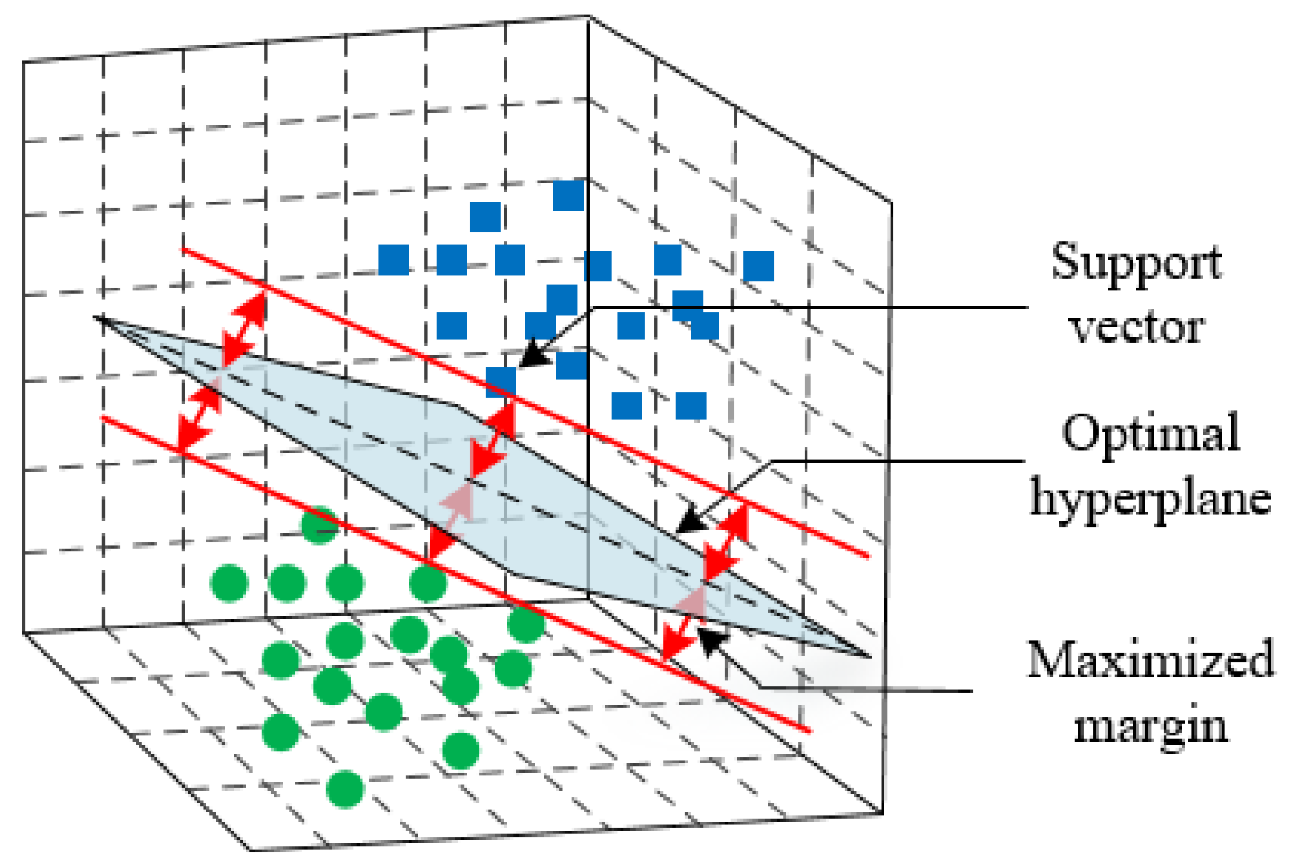
2. Support Vector Machine
3. OCC System Overview
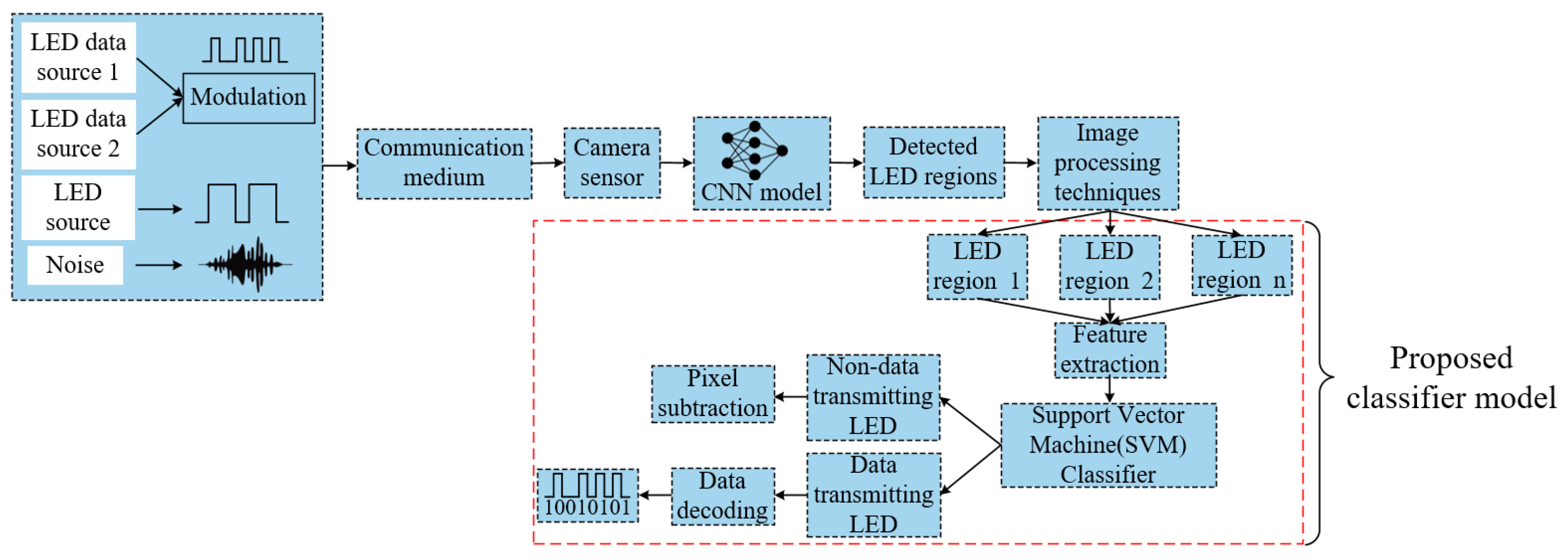
3.1. OCC System Architecture
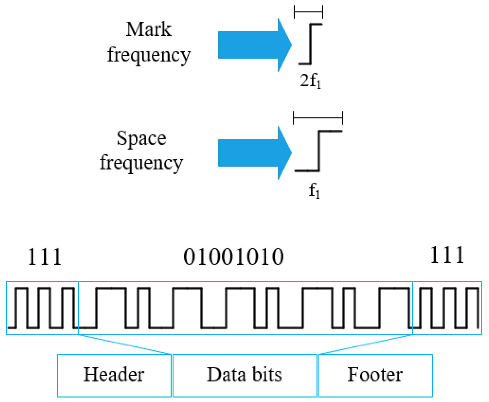
3.2. FSOOK Modulation
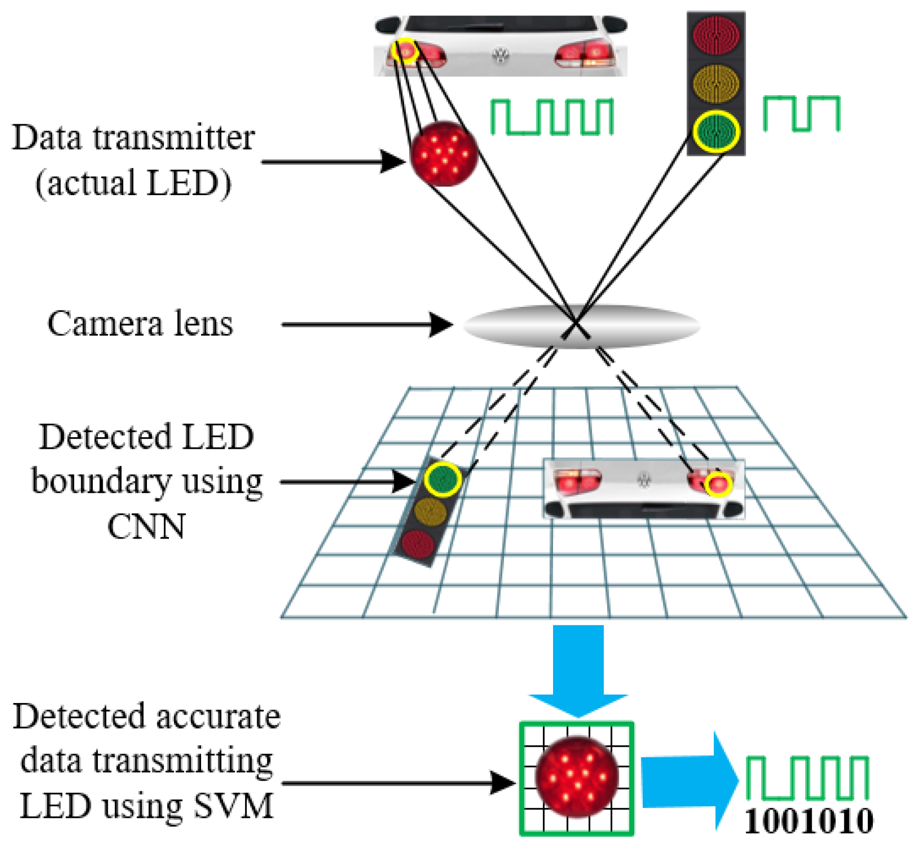
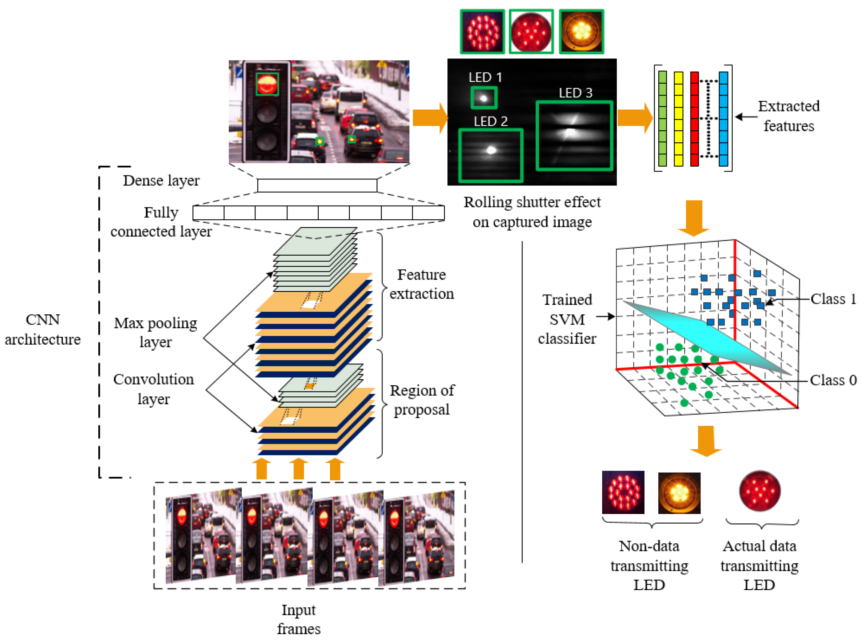
3.3. Proposed SVM Classifier Assisted Intelligent Receiver
3.3.1. LED Region Detection by a Convolutional Neural Network
3.3.2. Accurate Data Transmitting LED Region Separation
3.3.3. Data Decoding Method from the Accurate LED Region
| Algorithm 1 Demodulation Scheme at the Receiver. |
| Input: Captured image of all LEDs state. |
| Output: “11101011...” from accurate data transmitting LED region. |
| 1: read each RGB image ; |
| 2: detection of each LED region by CNN and separate regions ; |
| 3: convert to grayscale image ; |
| 4: draw contour on each of the ; |
| 5: for no. of separated LED region do |
| 6: extract features ; |
| 7: pass features to trained SVM classifier; |
| 8: recognize accurate data transmitting LED region; |
| 9: end for |
| 10: normalize each row intensities’ values ; |
| 11: set median of normalized values as threshold ; |
| 12: for do |
| 13: if then |
| 14: assign “1”; |
| 15: else |
| 16: assign “0”; |
| 17: end if |
| 18: calculate width of successive “0” and width of successive “0”; |
| 19: end for |
| 20: if then |
| 21: set “0”; |
| 22: else |
| 23: set “1”; |
| 24: end if |
4. Data Set Preparation
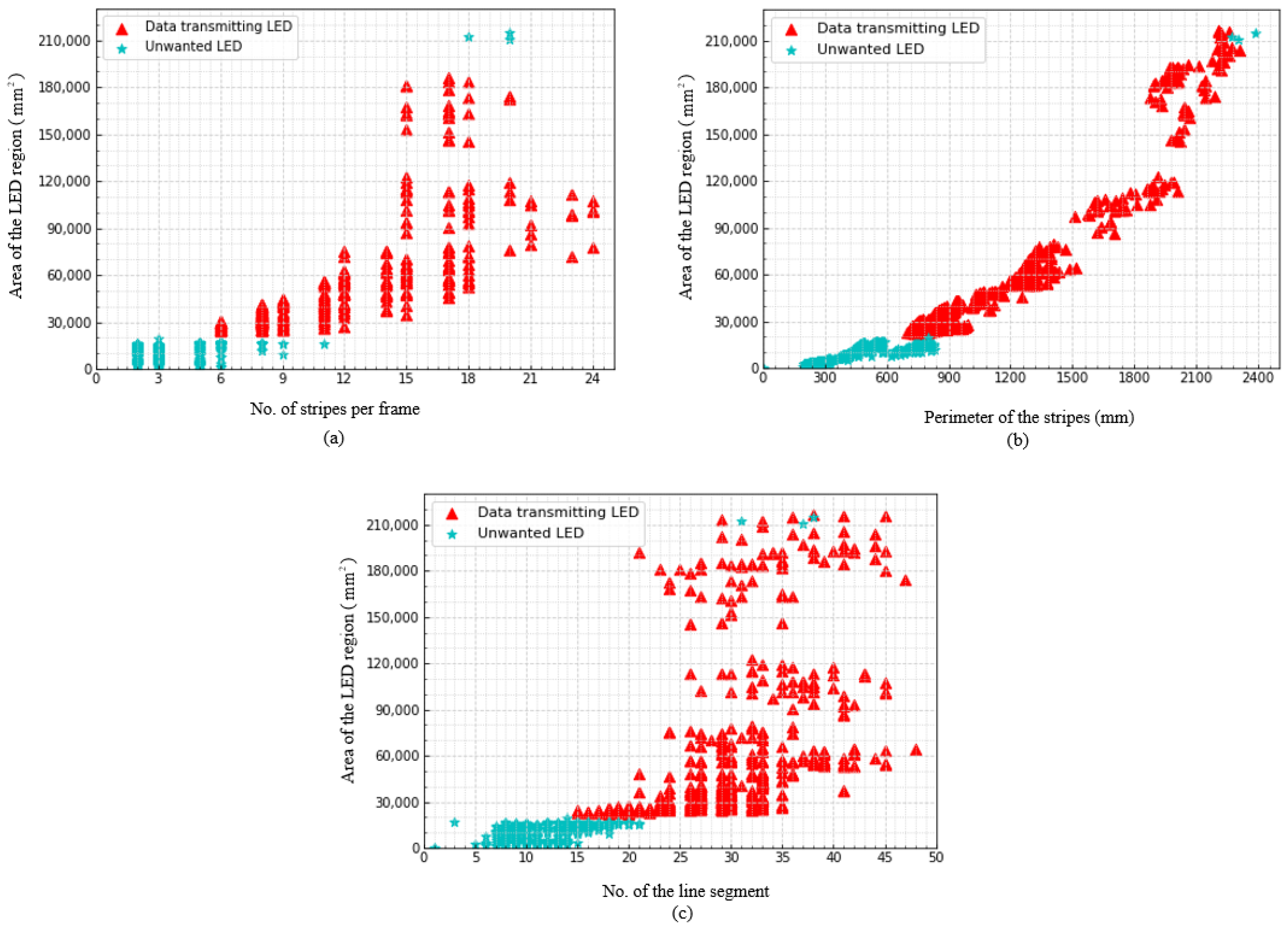
4.1. Zero Order Moments or Area of LED Region ()
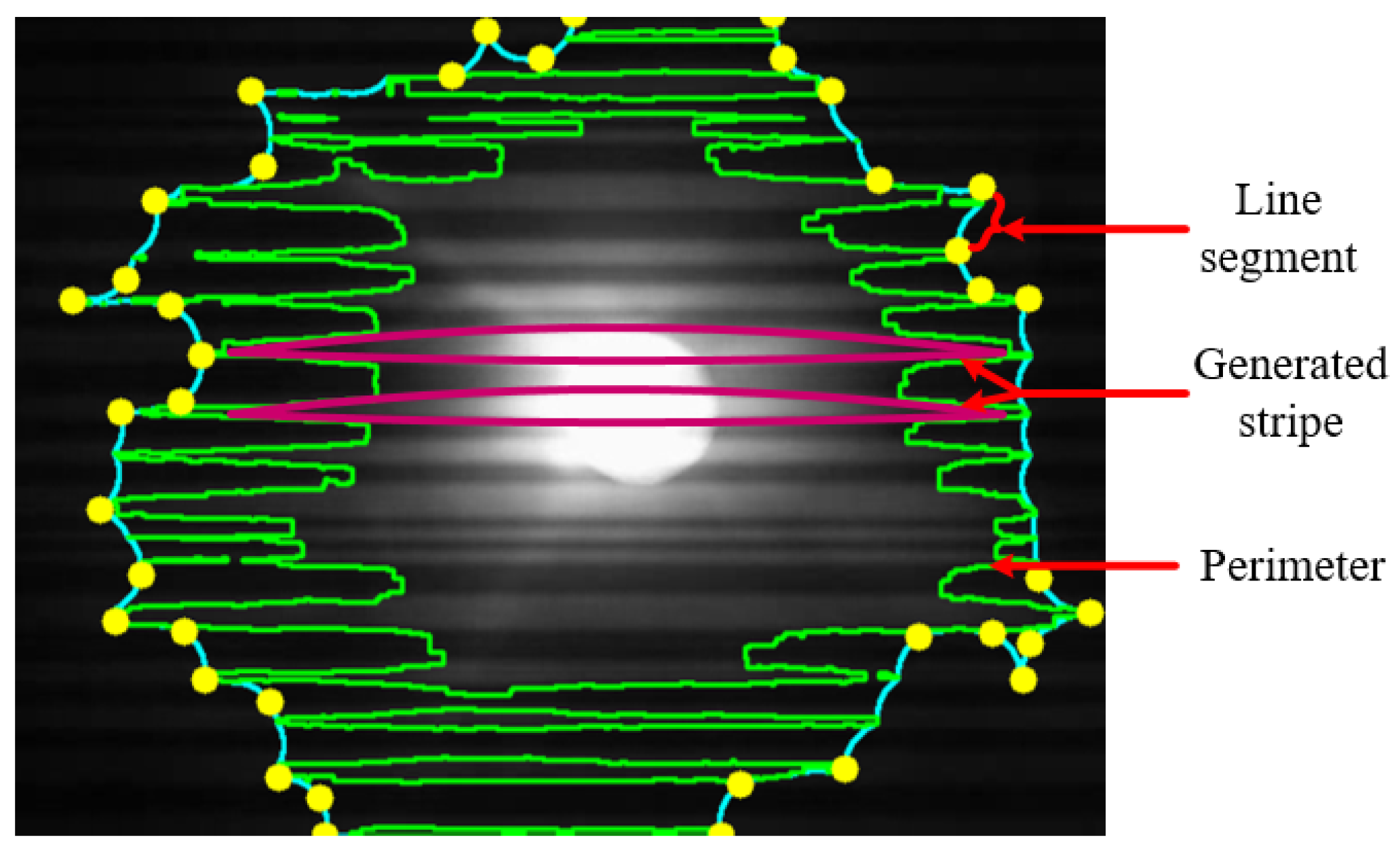
4.2. No. of Stripes per LED Region ()
4.3. Perimeter of Combined Stripes Contour ()
4.4. No. of Line Segment of Combined Stripes Contour ()
5. Experimental Results
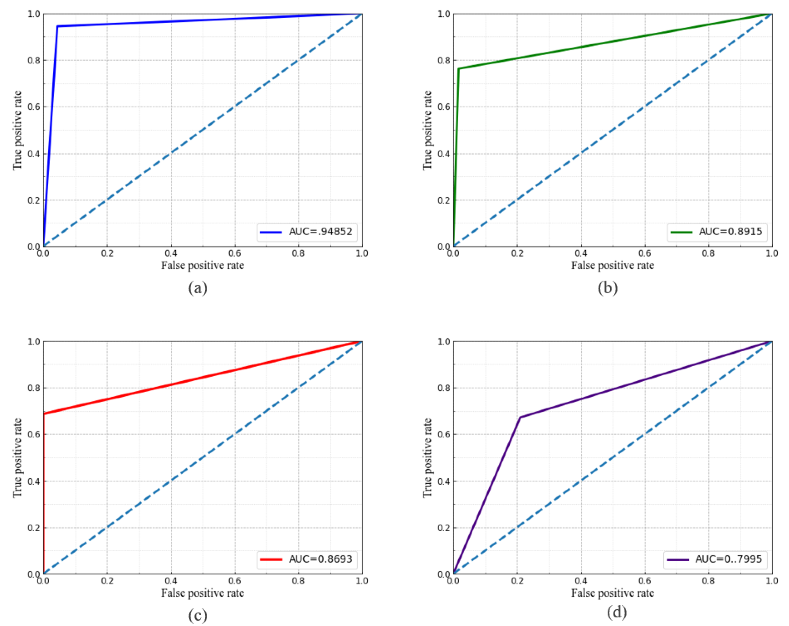
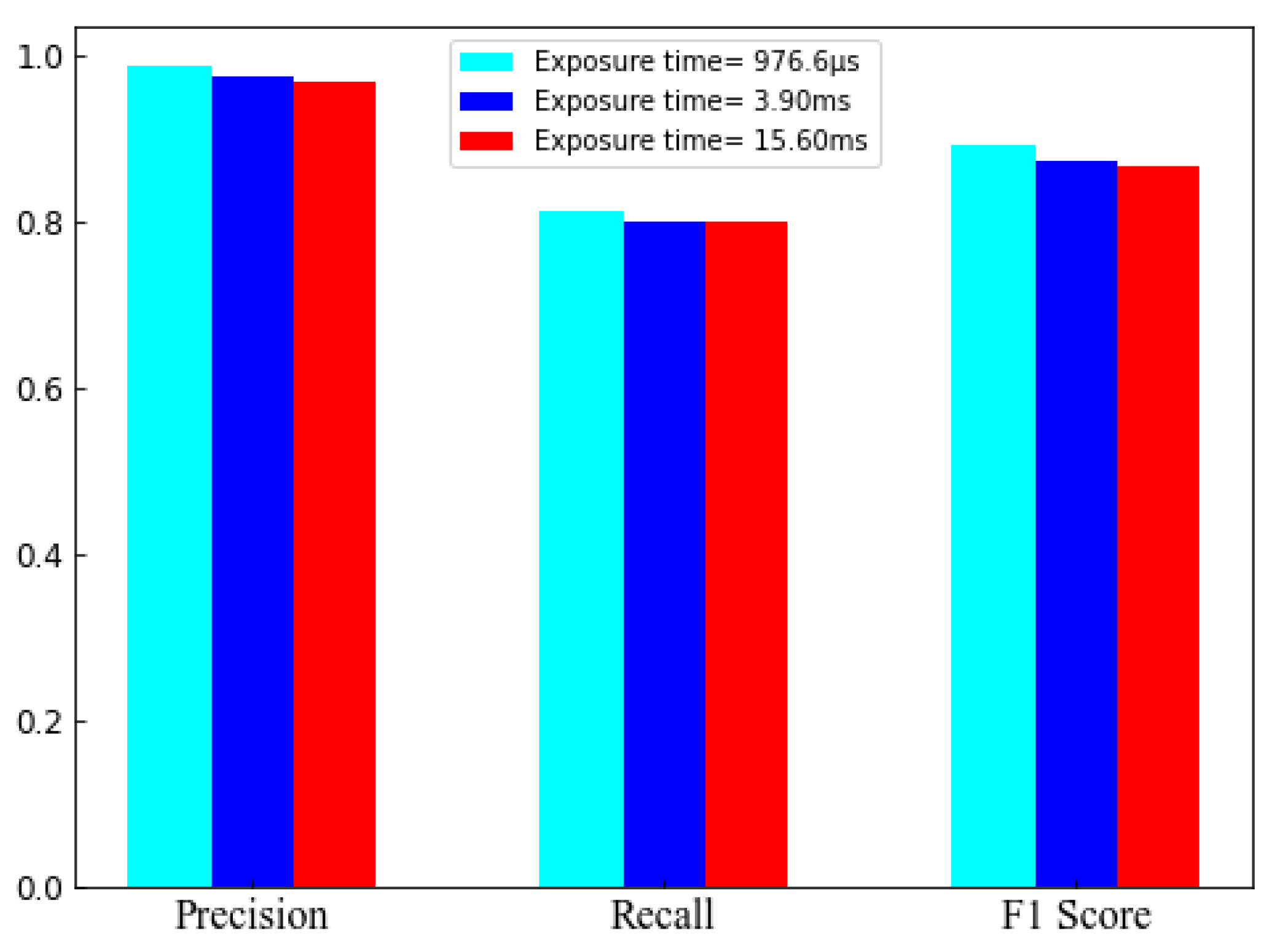
5.1. Classifier Performance
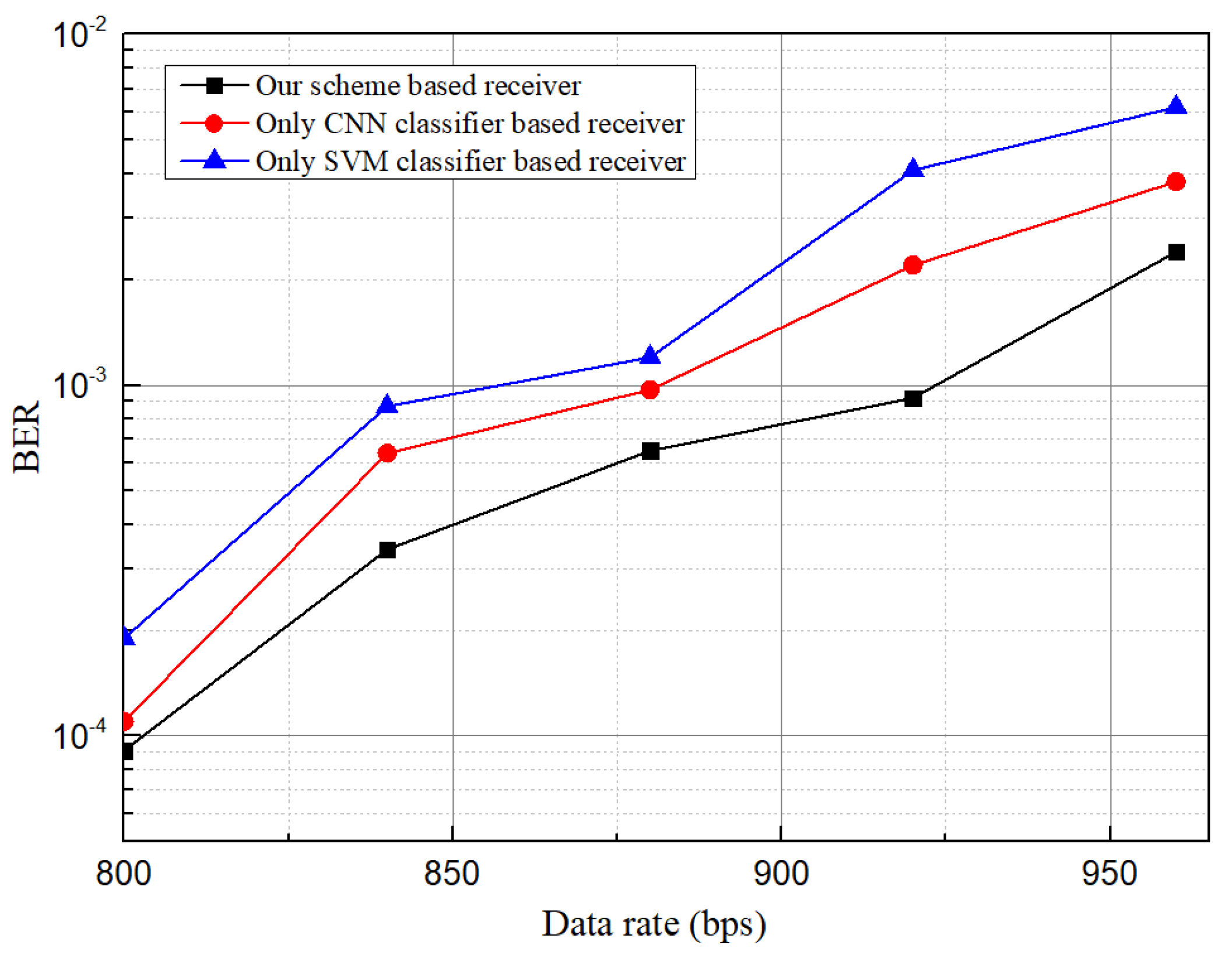
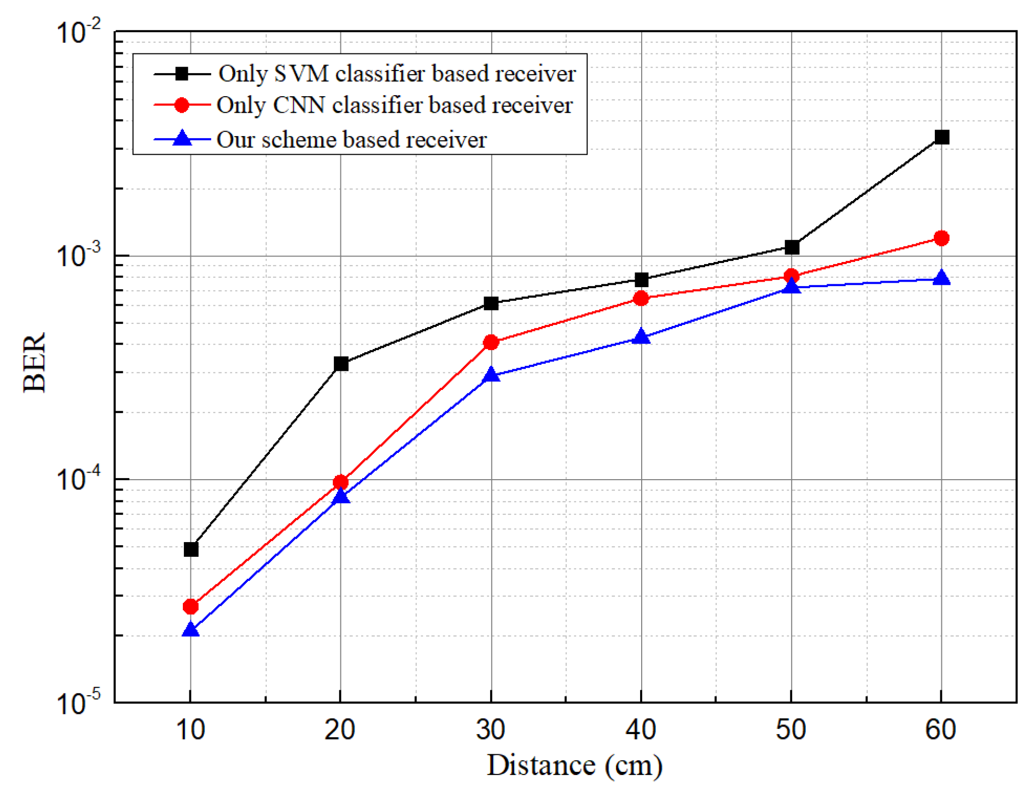
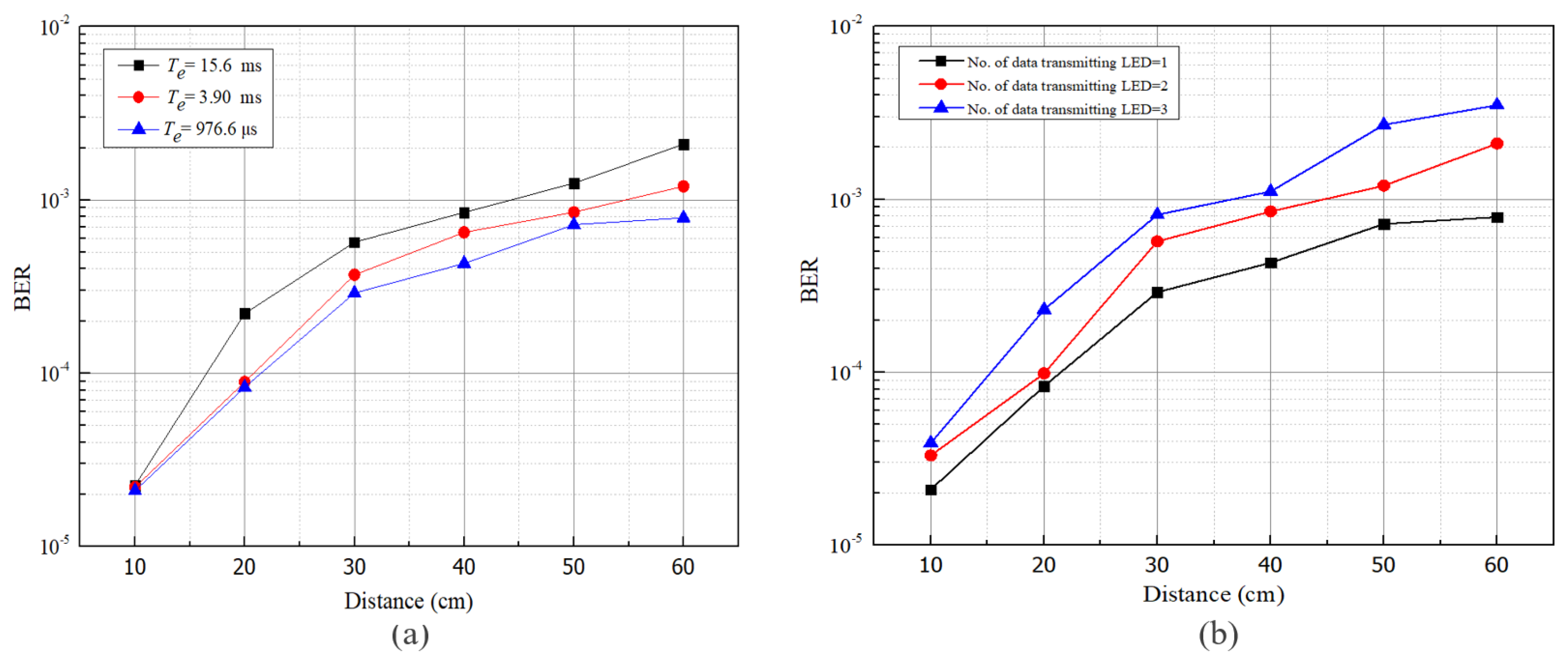
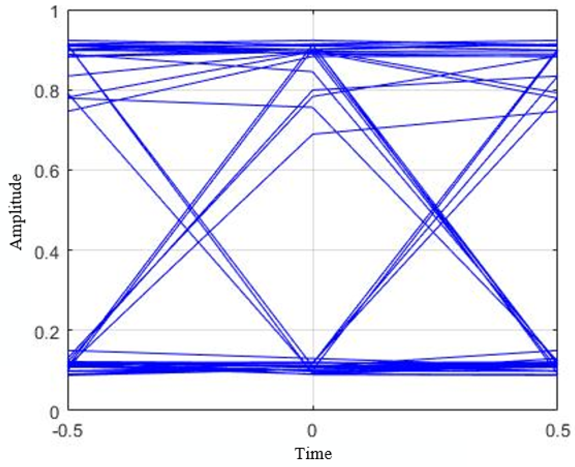
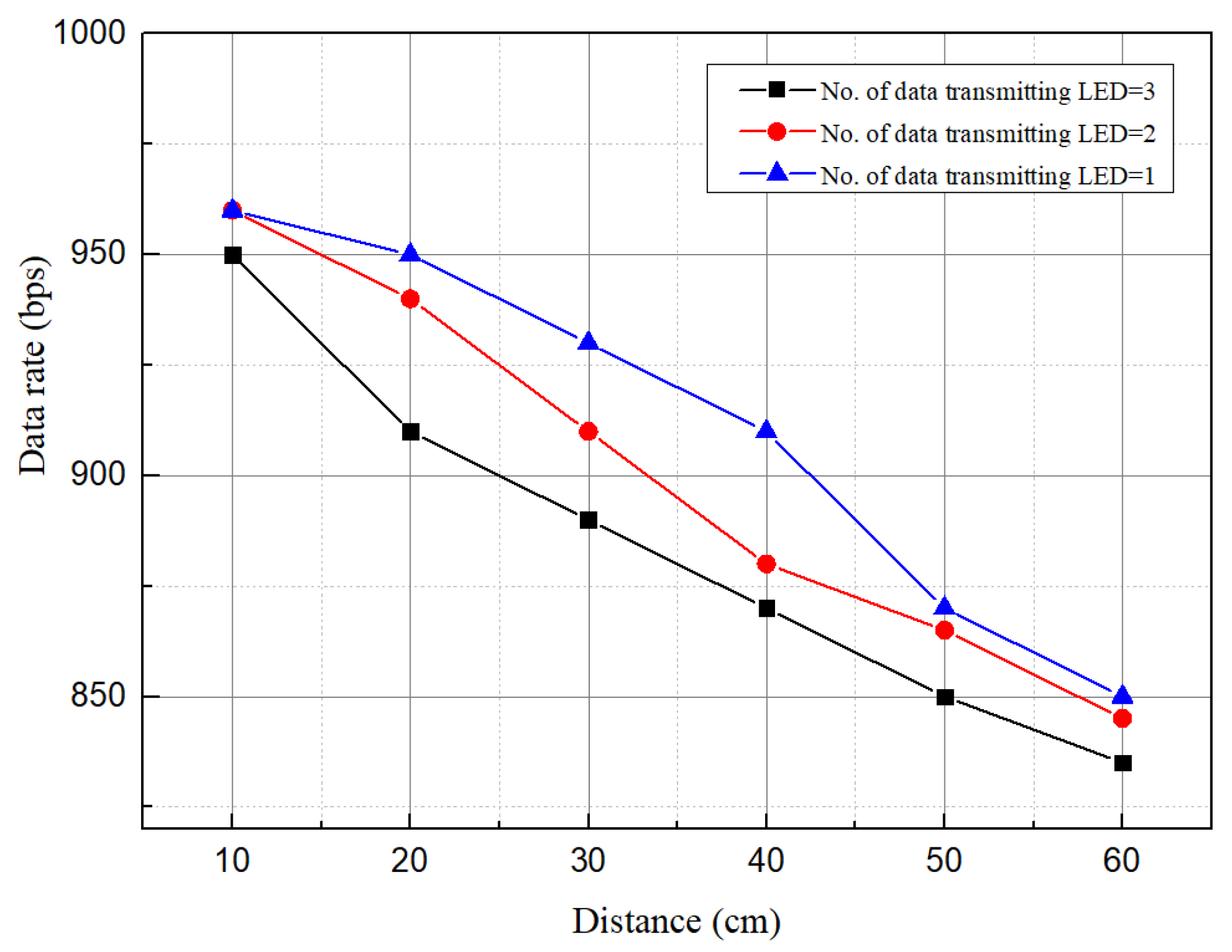
5.2. BER, Data Rate, and ISI Analysis
6. Conclusions
Author Contributions
Funding
Institutional Review Board Statement
Informed Consent Statement
Data Availability Statement
Conflicts of Interest
References
- Chow, C.W.; Yeh, C.H.; Liu, Y.; Liu, Y.F. Digital signal processing for light emitting diode based visible light communication. IEEE Photon. Soc. Newsl. 2012, 26, 9–13. [Google Scholar]
- Liao, C.-L.; Ho, C.-L.; Chang, Y.-F.; Wu, C.-H.; Wu, M.-C. High-speed light-emitting diodes emitting at 500 nm with 463-MHz modulation bandwidth. IEEE Electron. Device Lett. 2014, 35, 563–565. [Google Scholar] [CrossRef]
- Luo, P.; Zhang, M.; Ghassemlooy, Z.; Minh, H.L.; Tsai, H.-M.; Tang, X.; Png, L.C.; Han, D. Experimental demonstration of RGB LED-based optical camera communications. IEEE Photonics J. 2015, 7, 1–12. [Google Scholar] [CrossRef]
- Le, N.T.; Hossain, M.A.; Jang, Y.M. A survey of design and implementation for optical camera communication. Signal Process. Image Commun. 2017, 53, 95–109. [Google Scholar] [CrossRef]
- Yamazato, T.; Takai, I.; Okada, H.; Fujii, T.; Yendo, T.; Arai, S.; Andoh, M.; Harada, T.; Yasutomi, K.; Kagawa, K.; et al. Image-sensor-based visible light communication for automotive applications. IEEE Commun. Mag. 2014, 52, 88–97. [Google Scholar] [CrossRef]
- Chowdhury, M.Z.; Hasan, M.K.; Shahjalal, M.; Hossan, M.T.; Jang, Y.M. Optical wireless hybrid networks: Trends, opportunities, challenges, and research directions. IEEE Commun. Surv. Tutor. 2020, 22, 930–966. [Google Scholar] [CrossRef]
- Takai, I.; Harada, T.; Andoh, M.; Yasutomi, K.; Kagawa, K.; Kawahito, S. Optical vehicle-to-vehicle communication system using LED transmitter and camera receiver. IEEE Photonics J. 2014, 6, 1–14. [Google Scholar] [CrossRef]
- Chowdhury, M.Z.; Hossan, M.T.; Shahjalal, M.; Hasan, M.K.; Jang, Y.M. A new 5G eHealth architecture based on optical camera communication: An Overview, Prospects, and Applications. IEEE Consum. Electron. Mag. 2020, 9, 23–33. [Google Scholar] [CrossRef]
- Katz, M.; Ahmed, I. Opportunities and Challenges for Visible Light Communications in 6G. In Proceedings of the 2nd 6G Wireless Summit (6G SUMMIT), Levi, Finland, 17–20 March 2020. [Google Scholar]
- Marabissi, D.; Mucchi, L.; Caputo, S.; Nizzi, F.; Pecorella, T.; Fantacci, R.; Nawaz, T.; Seminara, M.; Catani, J. Experimental Measurements of a Joint 5G-VLC Communication for Future Vehicular Networks. J. Sens. Actuator Netw. 2020, 9, 32. [Google Scholar] [CrossRef]
- Pham, T.L.; Shahjalal, M.; Bui, V.; Jang, Y.M. Deep Learning for Optical Vehicular Communication. IEEE Access 2020, 8, 102691–102708. [Google Scholar] [CrossRef]
- Chen, Q.; Wen, H.; Deng, R.; Chen, M.; Geng, K. Spaced color shift keying modulation for camera-based visible light communication system using rolling shutter effect. Opt. Commun. 2019, 449, 19–23. [Google Scholar] [CrossRef]
- Roberts, R.D. Undersampled frequency shift ON-OFF keying (UFSOOK) for camera communications (CamCom). In Proceedings of the 22nd Wireless and Optical Communication Conference, Chongqing, China, 16–18 May 2013. [Google Scholar]
- Liu, N.; Cheng, J.; Holzman, J.F. Undersampled differential phase shift on-off keying for optical camera communications. J. Commun. Netw. 2017, 2, 47–56. [Google Scholar] [CrossRef] [Green Version]
- Monteiro, E.; Hranilovic, S. Design and implementation of color-shift keying for visible light communications. J. Lightwave Technol. 2014, 32, 2053–2060. [Google Scholar] [CrossRef] [Green Version]
- Rachim, V.P.; Chung, W.-Y. Multilevel intensity-modulation for rolling shutter-based optical camera communication. IEEE Photonics Technol. Lett. 2018, 30, 903–906. [Google Scholar] [CrossRef]
- Islam, A.; Hossan, M.T.; Jang, Y.M. Convolutional neural networkscheme–based optical camera communication system for intelligent Internet of vehicles. Int. J. Distrib. Sens. Netw. 2018, 14, 1550147718770153. [Google Scholar] [CrossRef]
- Yu, K.; He, J.; Huang, Z. Decoding scheme based on CNN for mobile optical camera communication. Appl. Opt. 2020, 59, 7109–7113. [Google Scholar] [CrossRef]
- Hasan, M.K.; Chowdhury, M.Z.; Shahjalal, M.; Nguyen, V.T.; Jang, Y.M. Performance analysis and improvement of optical camera communication. Appl. Sci. 2018, 8, 2527. [Google Scholar] [CrossRef] [Green Version]
- Nagura, T.; Yamazato, T.; Katayama, M.; Yendo, T.; Fujii, T.; Okada, H. Improved decoding methods of visible light communication system for ITS using LED array and high-speed camera. In Proceedings of the IEEE 71st Vehicular Technology Conference, Taipei, Taiwan, 16–19 May 2010. [Google Scholar]
- Chi, N.; Jia, J.; Hu, F.; Zhao, Y.; Zou, P. Challenges and prospects of machine learning in visible light communication. J. Commun. Inf. Netw. 2020, 5, 302–309. [Google Scholar]
- Yuan, Y.; Zhang, M.; Luo, P. SVM-based detection in visible light communications. Optik 2017, 151, 55–64. [Google Scholar] [CrossRef]
- Li, J.; Guan, W. The optical barcode detection and recognition method based on visible light communication using machine learning. Appl. Sci. 2018, 8, 2425. [Google Scholar] [CrossRef] [Green Version]
- Niu, W.; Ha, Y.; Chi, N. Support vector machine based machine learning method for GS 8QAM constellation classification in seamless integrated fiber and visible light communication system. Sci. China Inf. Sci. 2020, 63, 202306. [Google Scholar] [CrossRef]
- Dosovitskiy, A.; Beyer, L.; Kolesnikov, A.; Weissenborn, D.; Houlsby, N. An image is worth 16 × 16 words: Transformers for image recognition at scale. In Proceedings of the International Conference on Learning Representation, Virtual Conference, Vienna, Austria, 3–7 May 2021. [Google Scholar]
- Yamga, G.M.M.; Ndjiongue, A.R.; Ouahada, K. Low complexity clipped Frequency Shift Keying (FSK) for Visible Light Communications. In Proceedings of the IEEE 7th International Conference on Adaptive Science & Technology (ICAST), Accra, Ghana, 22–24 August 2018. [Google Scholar]
- Bazi, Y.; Melgani, F. Toward an optimal SVM classification system for hyperspectral remote sensing images. IEEE Trans. Geosci. Remote Sens. 2006, 44, 3374–3385. [Google Scholar] [CrossRef]
- Brereton, R.G.; Lloyd, G.R. Support vector machines for classification and regression. Analyst 2010, 135, 230–267. [Google Scholar] [CrossRef]
- Chavez-Burbano, P.; Rabadan, J.; Guerra, V.; Perez-Jimenez, R. Flickering-Free Distance-Independent Modulation Scheme for OCC. Electronics 2021, 10, 1103. [Google Scholar] [CrossRef]
- Li, P.; Zhao, W. Image fire detection algorithms based on convolutional neural networks. Case Stud. Therm. Eng. 2020, 19, 100625. [Google Scholar] [CrossRef]
- Pedronette, D.C.G.; Torres, R. Shape retrieval using contour features and distance optimization. In Proceedings of the International Conference on Computer Vision Theory and Applications, Angers, France, 17–21 May 2010. [Google Scholar]
- Vincent, L. Morphological transformations of binary images with arbitrary structuring elements. Signal Process. 1991, 22, 3–23. [Google Scholar] [CrossRef]
- Ashtputre, S.; Sharma, M.; Ramaiya, M. Image segmentation based on moments and color map. In Proceedings of the International Conference on Communication Systems and Network Technologies, Gwalior, India, 5–8 April 2013. [Google Scholar]
- Douglas, D.H.; Peucker, T.K. Algorithms for the reduction of the number of points required to represent a digitized line or its caricature. Cartogr. Int. J. Geogr. Inf. Geovis. 1973, 10, 112–122. [Google Scholar] [CrossRef] [Green Version]


| Type | Function |
|---|---|
| Linear | |
| Radial basis function (RBF) | |
| Polynomial | |
| Sigmoid |
| Parameter | Value |
|---|---|
| LED diameter | 10 mm |
| Camera exposure time | ms, ms, and s |
| Camera frame rate | 30 fps |
| Camera image resolution | |
| Mark and space frequency | 4000 kHz and 2000 kHz |
| Learning rate | |
| No. of epoch | 30 |
| Kernels | RBF, linear, polynomial, and sigmoid |
| No. of Data Transmitting LED | Linear | RBF | Polynomial | Sigmoid | |
|---|---|---|---|---|---|
| One | Accuracy (%) | 92.09 | 94.92 | 89.45 | 80.93 |
| AUC | 0.89 | 0.94 | 0.87 | 0.79 | |
| Two | Accuracy (%) | 90.05 | 93.10 | 87.91 | 81.36 |
| AUC | 0.85 | 0.91 | 0.83 | 0.81 | |
| Three | Accuracy (%) | 87.76 | 89.91 | 88.13 | 79.87 |
| AUC | 0.84 | 0.88 | 0.85 | 0.77 |
Publisher’s Note: MDPI stays neutral with regard to jurisdictional claims in published maps and institutional affiliations. |
© 2021 by the authors. Licensee MDPI, Basel, Switzerland. This article is an open access article distributed under the terms and conditions of the Creative Commons Attribution (CC BY) license (https://creativecommons.org/licenses/by/4.0/).
Share and Cite
Rahman, M.H.; Shahjalal, M.; Hasan, M.K.; Ali, M.O.; Jang, Y.M. Design of an SVM Classifier Assisted Intelligent Receiver for Reliable Optical Camera Communication. Sensors 2021, 21, 4283. https://doi.org/10.3390/s21134283
Rahman MH, Shahjalal M, Hasan MK, Ali MO, Jang YM. Design of an SVM Classifier Assisted Intelligent Receiver for Reliable Optical Camera Communication. Sensors. 2021; 21(13):4283. https://doi.org/10.3390/s21134283
Chicago/Turabian StyleRahman, Md. Habibur, Md. Shahjalal, Moh. Khalid Hasan, Md. Osman Ali, and Yeong Min Jang. 2021. "Design of an SVM Classifier Assisted Intelligent Receiver for Reliable Optical Camera Communication" Sensors 21, no. 13: 4283. https://doi.org/10.3390/s21134283
APA StyleRahman, M. H., Shahjalal, M., Hasan, M. K., Ali, M. O., & Jang, Y. M. (2021). Design of an SVM Classifier Assisted Intelligent Receiver for Reliable Optical Camera Communication. Sensors, 21(13), 4283. https://doi.org/10.3390/s21134283