
A Monocular Visual Odometry Method Based on Virtual-Real Hybrid Map in Low-Texture Outdoor Environment


Abstract
1. Introduction
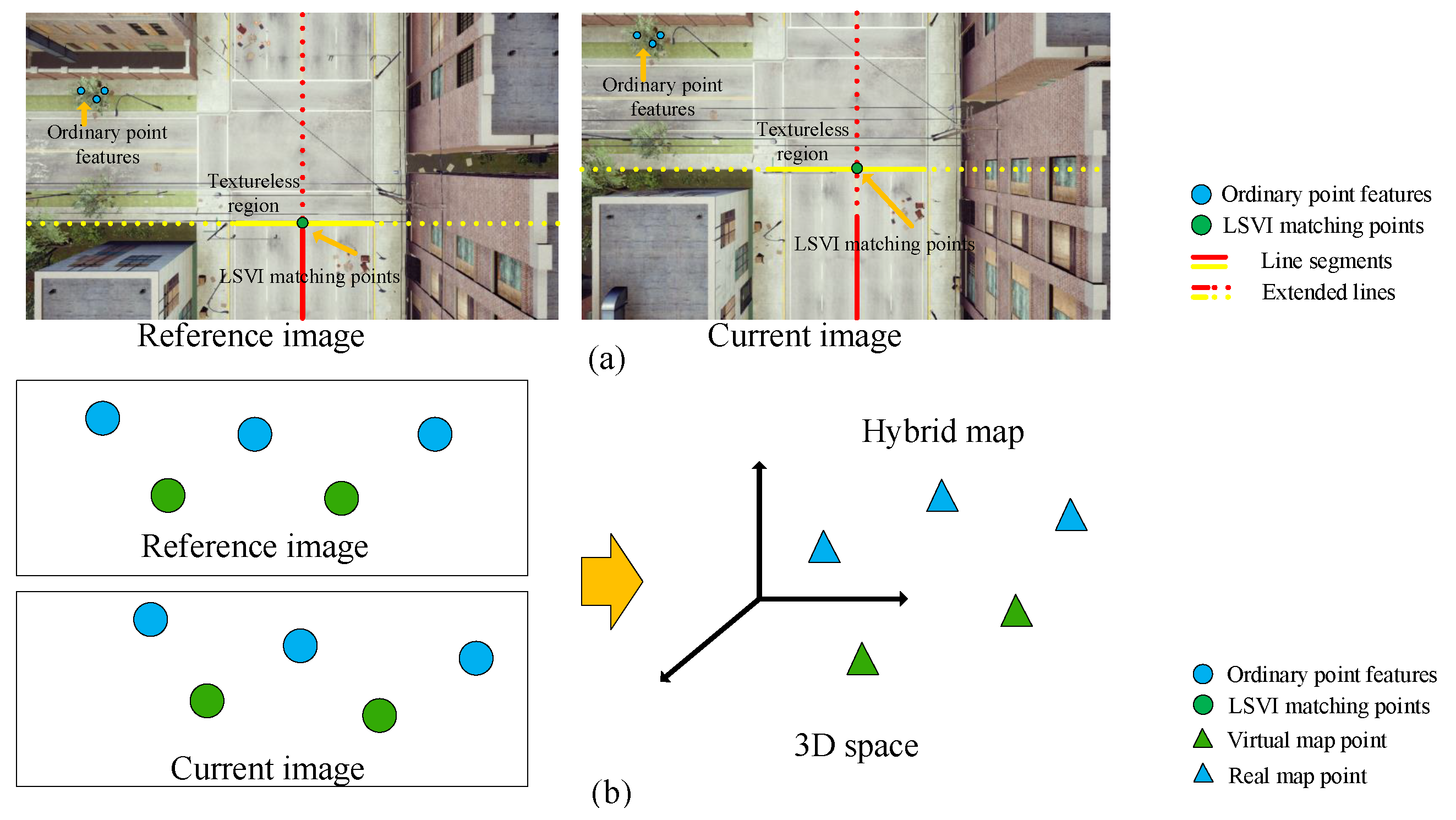
- First, we reprocess line segment features by combining line segments and introduce the concept of virtual intersection matching points.
- Second, we propose the concept of a virtual map using the line segment-based virtual intersection matching points and demonstrate that the virtual map can play the same role as the real map constructed by ordinary point features to participate in camera pose estimation.
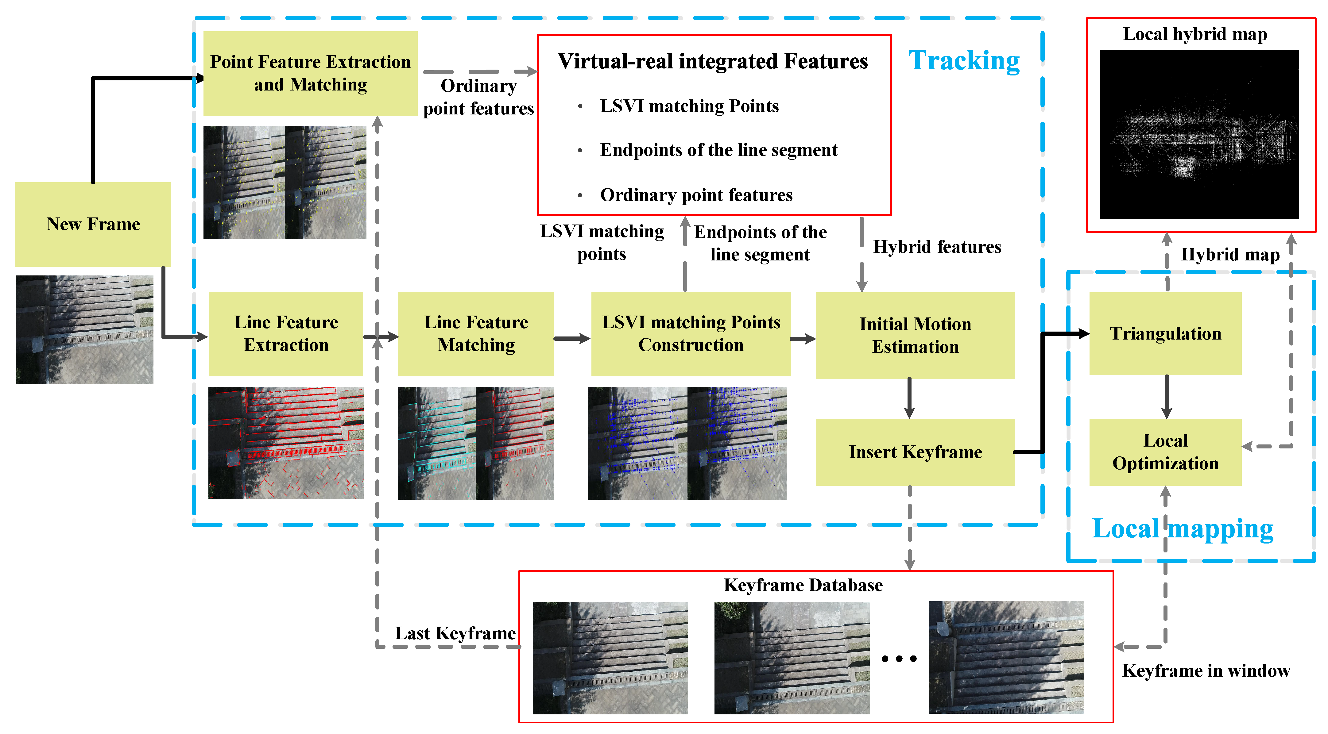
- Third, we propose a monocular VO algorithm based on the virtual-real hybrid map, as shown in Figure 1b, which is built on virtual intersection matching points, endpoints of line segments, and ordinary point features.
2. LSVI Matching Points
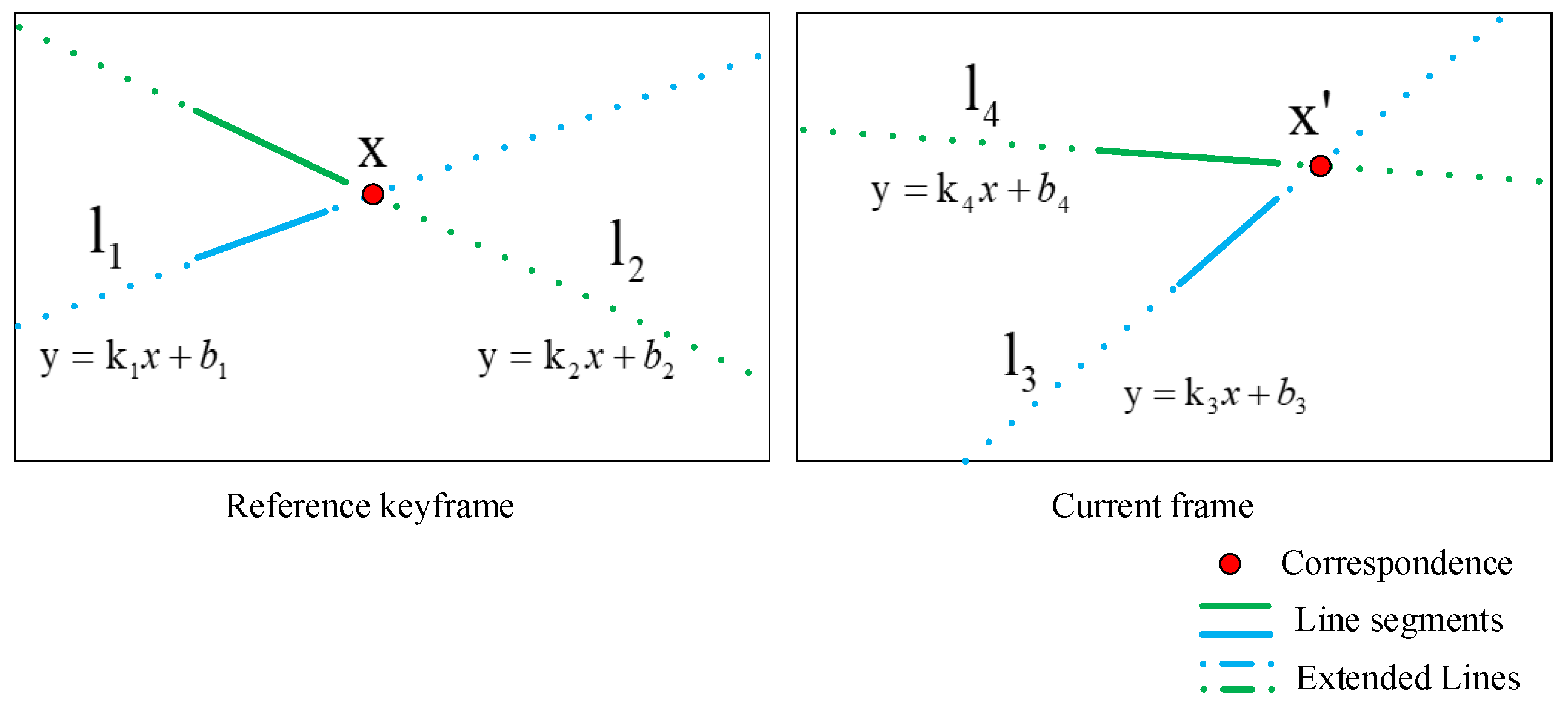
2.1. Definition
2.2. Virtual Map
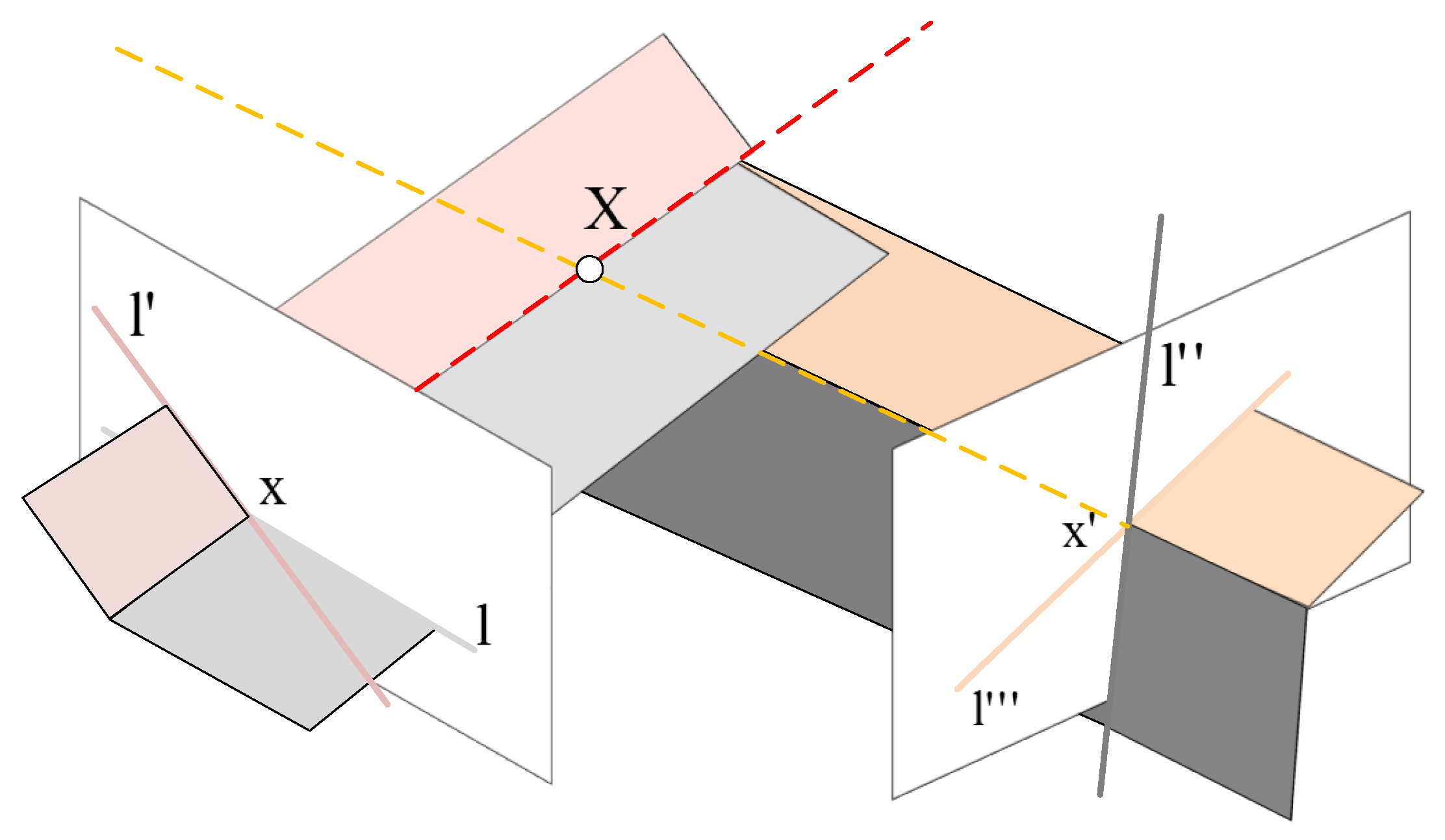
2.3. Demonstration
2.4. Significance of Introducing LSVI Matching Points
3. Virtual-Real Integrated VO Algorithm
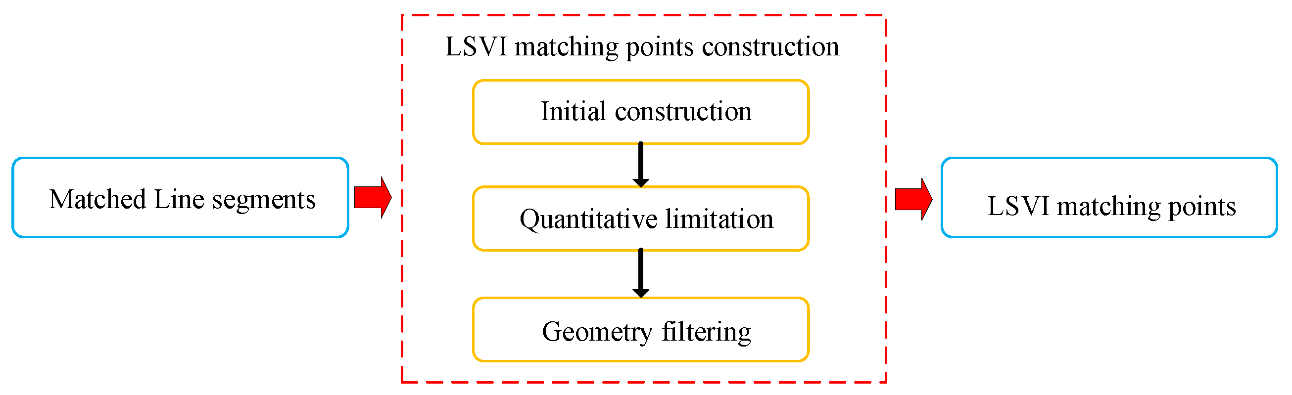
3.1. LSVI Matching Points Construction
3.2. Hybrid Map
3.3. Frame Management
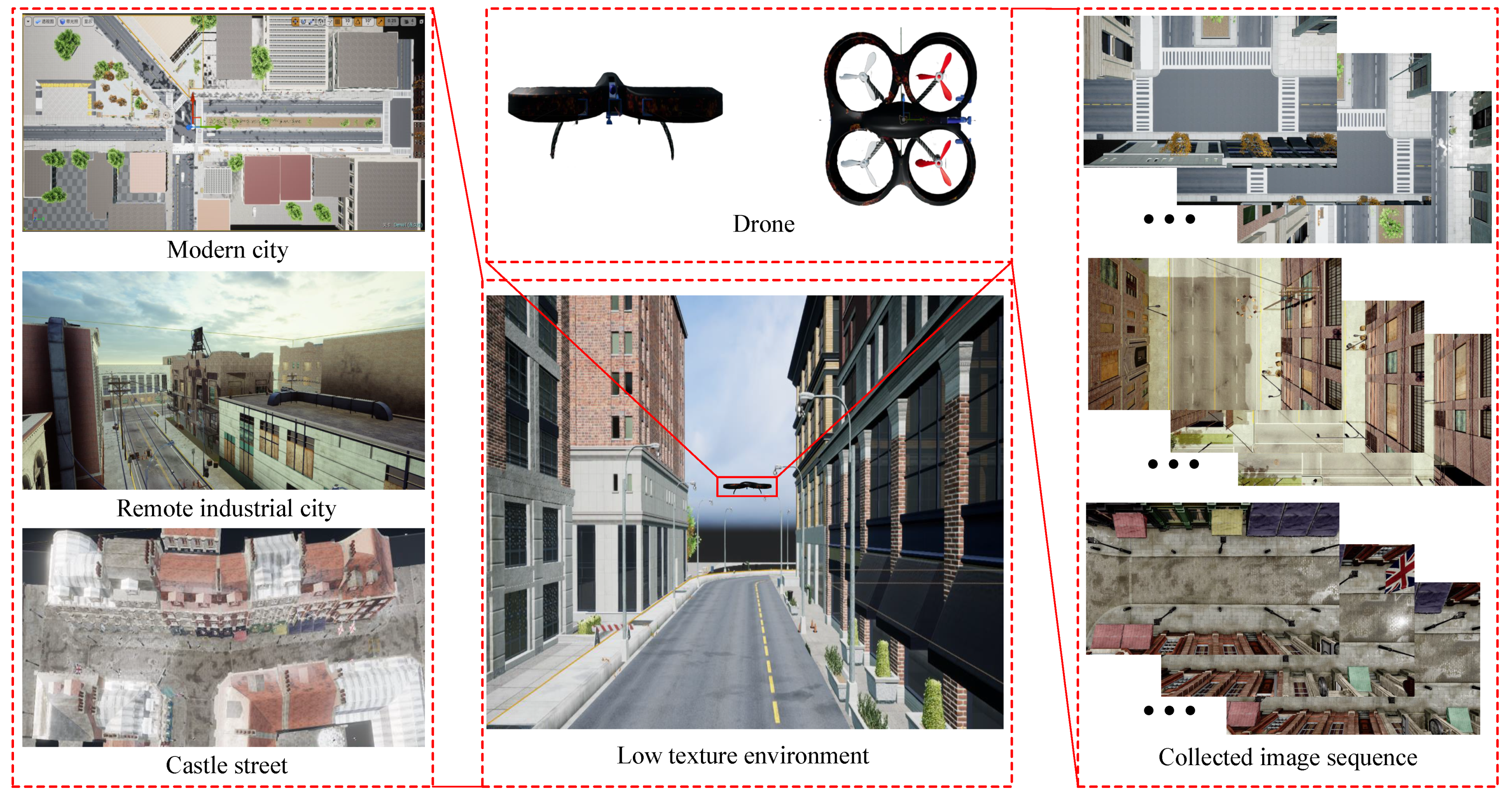
4. Results
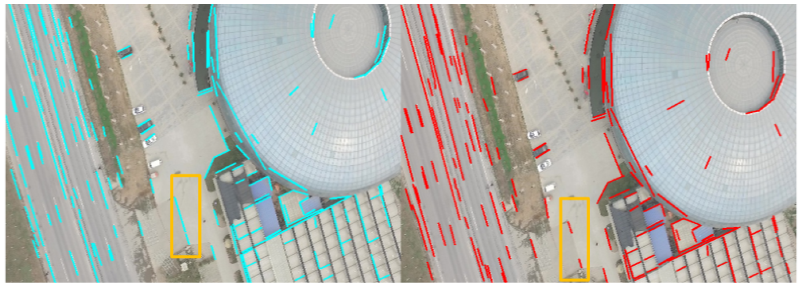
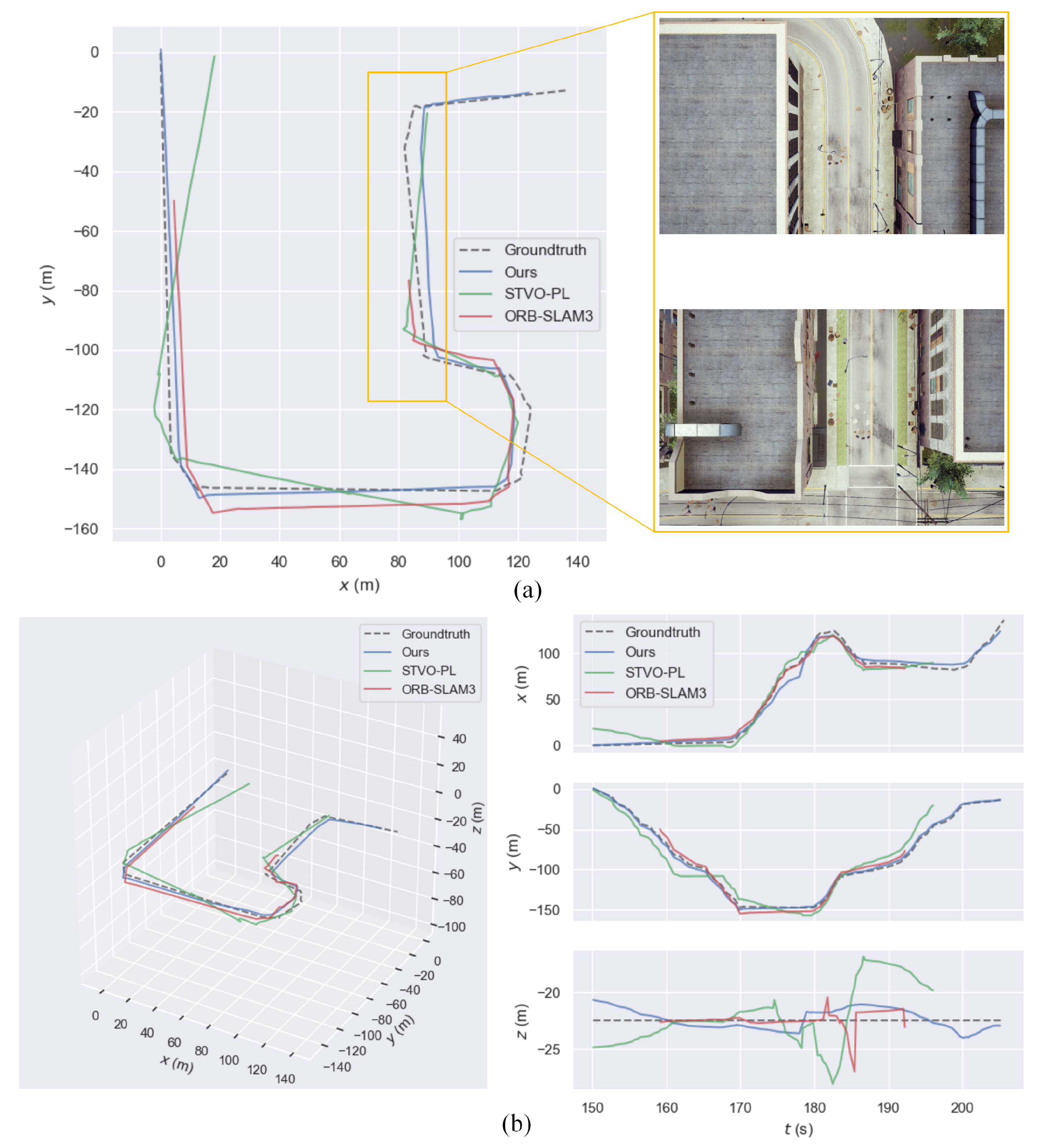
4.1. Qualitative Evaluation
4.2. Quantitative Evaluation
5. Discussion
6. Conclusions
Author Contributions
Funding
Institutional Review Board Statement
Informed Consent Statement
Data Availability Statement
Acknowledgments
Conflicts of Interest
Abbreviations
| VO | Visual odometry algorithm |
| SLAM | Simultaneous Localization and Mapping algorithm |
| UAV | Unmanned aerial vehicle |
| LSVI | Line segments based virtual intersection |
| GPU | Graphics Processing Unit |
| SIFT | Scale-invariant Feature Transform |
| DLT | Direct Linear Transformation |
| PnP | Perspective-n-Point |
| ORB | Oriented FAST and Rotated BRIEF |
| BRISK | Binary Robust Invariant Scalable Keypoints |
| EKF | Extended Kalman filter |
| PTAM | Parallel Tracking and Mapping |
| S-PTAM | Stereo Parallel Tracking and Mapping |
References
- Martin, P.G.; Connor, D.T.; Estrada, N.; El-Turke, A.; Megson-Smith, D.; Jones, C.P.; Kreamer, D.K.; Scott, T.B. Radiological Identification of Near-Surface Mineralogical Deposits Using Low-Altitude Unmanned Aerial Vehicle. Remote Sens. 2020, 12, 3562. [Google Scholar] [CrossRef]
- Zhang, Y.; Han, W.; Niu, X.; Li, G. Maize Crop Coefficient Estimated from UAV-Measured Multispectral Vegetation Indices. Sensors 2019, 19, 5250. [Google Scholar] [CrossRef] [PubMed]
- Huang, W.; Jiang, S.; Jiang, W. A Model-Driven Method for Pylon Reconstruction from Oblique UAV Images. Sensors 2020, 20, 824. [Google Scholar] [CrossRef] [PubMed]
- Liu, C.; Sziranyi, T. Real-Time Human Detection and Gesture Recognition for On-Board UAV Rescue. Sensors 2021, 21, 2180. [Google Scholar] [CrossRef]
- Yang, S.; Scherer, S.A.; Yi, X.; Zell, A. Multi-camera visual SLAM for autonomous navigation of micro aerial vehicles. Robot. Auton. Syst. 2017, 93, 116–134. [Google Scholar] [CrossRef]
- De la Escalera, A.; Izquierdo, E.; Martín, D.; Musleh, B.; García, F.; Armingol, J.M. Stereo visual odometry in urban environments based on detecting ground features. Robot. Auton. Syst. 2016, 80, 1–10. [Google Scholar] [CrossRef]
- Solin, A.; Cortes, S.; Rahtu, E.; Kannala, J. PIVO: Probabilistic Inertial-Visual Odometry for Occlusion-Robust Navigation. In Proceedings of the IEEE Winter Conference on Applications of Computer Vision, Lake Tahoe, NV, USA, 12–15 March 2018; pp. 616–625. [Google Scholar]
- Tateno, K.; Tombari, F.; Navab, N. Large scale and long standing simultaneous reconstruction and segmentation. Comput. Vis. Image Underst. 2017, 157, 138–150. [Google Scholar] [CrossRef]
- Engel, J.; Schöps, T.; Cremers, D. LSD-SLAM: Large-Scale Direct Monocular SLAM. In Proceedings of the European Conference on Computer Vision, Zurich, Switzerland, 06–12 September 2014; pp. 834–849. [Google Scholar]
- Engel, J.; Koltun, V.; Cremers, D. Direct sparse odometry. IEEE Trans. Pattern Anal. Mach. Intell. 2017, 40, 611–625. [Google Scholar] [CrossRef] [PubMed]
- Gao, X.; Wang, R.; Demmel, N.; Cremers, D. LDSO: Direct sparse odometry with loop closure. In Proceedings of the IEEE/RSJ International Conference on Intelligent Robots and Systems, Madrid, Spain, 1–5 October 2018; pp. 2198–2204. [Google Scholar]
- Klein, G.; Murray, D. Parallel tracking and mapping for small AR workspaces. In Proceedings of the IEEE and ACM International Symposium on Mixed and Augmented Reality, Nara, Japan, 13–16 November 2007; pp. 225–234. [Google Scholar]
- Pire, T.; Fischer, T.; Castro, G.; De Cristóforis, P.; Civera, J.; Berlles, J.J. S-PTAM: Stereo parallel tracking and mapping. Robot. Auton. Syst. 2017, 93, 27–42. [Google Scholar] [CrossRef]
- Mur-Artal, R.; Tardós, J.D. Orb-slam2: An open-source slam system for monocular, stereo, and rgb-d cameras. IEEE Trans. Robot. 2017, 33, 1255–1262. [Google Scholar] [CrossRef]
- Leutenegger, S.; Chli, M.; Siegwart, R.Y. BRISK: Binary robust invariant scalable keypoints. In Proceedings of the IEEE International Conference on Computer Vision, Barcelona, Spain, 6–13 November 2011; pp. 2548–2555. [Google Scholar]
- Rublee, E.; Rabaud, V.; Konolige, K.; Bradski, G. ORB: An efficient alternative to SIFT or SURF. In Proceedings of the IEEE International Conference on Computer Vision, Barcelona, Spain, 6–13 November 2011; pp. 2564–2571. [Google Scholar]
- Carlos, C.; Richard, E.; Juan, J.G.R.; José, M.M.M.; Juan, D.T. ORB-SLAM3: An Accurate Open-Source Library for Visual, Visual-Inertial and Multi-Map SLAM. arXiv 2020, arXiv:2007.11898. [Google Scholar]
- Pumarola, A.; Vakhitov, A.; Agudo, A.; Sanfeliu, A.; Moreno-Noguer, F. PL-SLAM: Real-time monocular visual SLAM with points and lines. In Proceedings of the IEEE International Conference on Robotics and Automation, Singapore, 29 May–3 June 2017; pp. 4503–4508. [Google Scholar]
- Eade, E.; Drummond, T. Edge landmarks in monocular SLAM. Image Vis. Comput. 2009, 27, 588–596. [Google Scholar] [CrossRef]
- Zhou, H.; Zou, D.; Pei, L.; Ying, R.; Liu, P.; Yu, W. StructSLAM: Visual SLAM with building structure lines. IEEE Trans. Veh. Technol. 2015, 64, 1364–1375. [Google Scholar] [CrossRef]
- Vakhitov, A.; Funke, J.; Moreno-Noguer, F. Accurate and linear time pose estimation from points and lines. In Proceedings of the European Conference on Computer Vision, Amsterdam, The Netherlands, 8–16 October 2016; pp. 583–599. [Google Scholar]
- Gomez-Ojeda, R.; Gonzalez-Jimenez, J. Robust stereo visual odometry through a probabilistic combination of points and line segments. In Proceedings of the IEEE International Conference on Robotics and Automation, Stockholm, Sweden, 16–21 May 2016; pp. 2521–2526. [Google Scholar]
- Gomez-Ojeda, R.; Moreno, F.A.; Zuñiga-Noël, D.; Scaramuzza, D.; Gonzalez-Jimenez, J. PL-SLAM: A stereo SLAM system through the combination of points and line segments. IEEE Trans. Robot. 2019, 35, 734–746. [Google Scholar] [CrossRef]
- Yang, S.; Song, Y.; Kaess, M.; Scherer, S. Pop-up SLAM: Semantic Monocular Plane SLAM for Low-texture Environments. In Proceedings of the IEEE/RSJ International Conference on Intelligent Robots and Systems, Daejeon, Korea, 9–14 October 2016; pp. 1222–1229. [Google Scholar]
- Yang, S.; Maturana, D.; Scherer, S. Real-time 3D Scene Layout from a Single Image Using Convolutional Neural Networks. In Proceedings of the IEEE International Conference on Robotics and Automation, Stockholm, Sweden, 16–21 May 2016; pp. 2183–2189. [Google Scholar]
- Fu, Q.; Yu, H.; Lai, L.; Wang, J.; Peng, X.; Sun, W.; Sun, M. A Robust RGB-D SLAM System With Points and Lines for Low Texture Indoor Environments. IEEE Sens. J. 2019, 19, 9908–9920. [Google Scholar] [CrossRef]
- Fabian, S.; Friedrich, F. Combining Edge Images and Depth Maps for Robust Visual Odometry. In Proceedings of the British Machine Vision Conference, London, UK, 4–7 September 2017; pp. 1–12. [Google Scholar]
- Hartley, R.; Zisserman, A. Multiple View Geometry in Computer Vision; Cambridge University Press: Cambridge, UK, 2003. [Google Scholar]
- Lepetit, V.; Moreno-Noguer, F.; Fua, P. EPnP: An Accurate O(n) Solution to the PnP Problem. Int. J. Comput. Vis. 2009, 81, 155–166. [Google Scholar] [CrossRef]
- Schönberger, J.L.; Frahm, J. Structure-from-Motion Revisited. In Proceedings of the IEEE Conference on Computer Vision and Pattern Recognition, Las Vegas, NV, USA, 27–30 June 2016; pp. 4104–4113. [Google Scholar]
- Triggs, B.; McLauchlan, P.F.; Hartley, R.I.; Fitzgibbon, A.W. Bundle adjustment—A modern synthesis. In Proceedings of the International Workshop on Vision Algorithms, Corfu, Greece, 21–22 September 1999; pp. 298–372. [Google Scholar]
- Von Gioi, R.G.; Jakubowicz, J.; Morel, J.M.; Randall, G. LSD: A fast line segment detector with a false detection control. IEEE Trans. Pattern Anal. Mach. Intell. 2008, 32, 722–732. [Google Scholar] [CrossRef] [PubMed]
- Zhang, L.; Koch, R. An efficient and robust line segment matching approach based on LBD descriptor and pairwise geometric consistency. J. Vis. Commun. Image Represent. 2013, 24, 794–805. [Google Scholar] [CrossRef]
- Wu, C. A GPU Implementation of Scale Invariant Feature Transform (SIFT). Available online: https://github.com/pitzer/SiftGPU (accessed on 10 February 2021).
- Nocedal, J.; Wright, S. Numerical Optimization, 2nd ed.; Springer: Berlin, Germany, 2006. [Google Scholar]
- Kümmerle, R.; Grisetti, G.; Strasdat, H.; Konolige, K.; Burgard, W. g2o: A general framework for graph optimization. In Proceedings of the IEEE International Conference on Robotics and Automation, Shanghai, China, 9–13 May 2011; pp. 3607–3613. [Google Scholar]
- Shah, S.; Kapoor, A.; Dey, D.; Lovett, C. AirSim: High-Fidelity Visual and Physical Simulation for Autonomous Vehicles. Field Serv. Robot. 2017, 5, 621–635. [Google Scholar]
- Grupp, M. evo: Python Package for the Evaluation of Odometry and SLAM. Available online: https://github.com/MichaelGrupp/evo (accessed on 10 February 2021).


| Methods | IndustrialCity-d | CastleStreet-d | CastleStreet-f | ModernCity-d |
|---|---|---|---|---|
| ORB-SLAM3 | 9.501 | 0.491 | 0.129 | 2.124 |
| DSO | x | x | x | x |
| STVO-PL | 13.90 | 1.787 | 0.662 | 4.517 |
| Ours | 5.186 | 0.467 | 0.199 | 1.384 |
| Thread | Operation | Time (ms) |
|---|---|---|
| Tracking | Feature detection | 39.1 |
| Feature matching | 2.84 | |
| LSVI matching points construction | 3.98 | |
| Initial motion estimation | 4.13 | |
| Total tracking | 51.1 | |
| Local mapping | Triangulation | 13.7 |
| BA | 51.4 | |
| Total mapping | 65.1 | |
| Total mean | 56.2 | |
Publisher’s Note: MDPI stays neutral with regard to jurisdictional claims in published maps and institutional affiliations. |
© 2021 by the authors. Licensee MDPI, Basel, Switzerland. This article is an open access article distributed under the terms and conditions of the Creative Commons Attribution (CC BY) license (https://creativecommons.org/licenses/by/4.0/).
Share and Cite
Xie, X.; Yang, T.; Ning, Y.; Zhang, F.; Zhang, Y. A Monocular Visual Odometry Method Based on Virtual-Real Hybrid Map in Low-Texture Outdoor Environment. Sensors 2021, 21, 3394. https://doi.org/10.3390/s21103394
Xie X, Yang T, Ning Y, Zhang F, Zhang Y. A Monocular Visual Odometry Method Based on Virtual-Real Hybrid Map in Low-Texture Outdoor Environment. Sensors. 2021; 21(10):3394. https://doi.org/10.3390/s21103394
Chicago/Turabian StyleXie, Xiuchuan, Tao Yang, Yajia Ning, Fangbing Zhang, and Yanning Zhang. 2021. "A Monocular Visual Odometry Method Based on Virtual-Real Hybrid Map in Low-Texture Outdoor Environment" Sensors 21, no. 10: 3394. https://doi.org/10.3390/s21103394
APA StyleXie, X., Yang, T., Ning, Y., Zhang, F., & Zhang, Y. (2021). A Monocular Visual Odometry Method Based on Virtual-Real Hybrid Map in Low-Texture Outdoor Environment. Sensors, 21(10), 3394. https://doi.org/10.3390/s21103394