Improving the Resolution and Accuracy of Groundwater Level Anomalies Using the Machine Learning-Based Fusion Model in the North China Plain


Abstract
1. Introduction
2. Study Area and Data
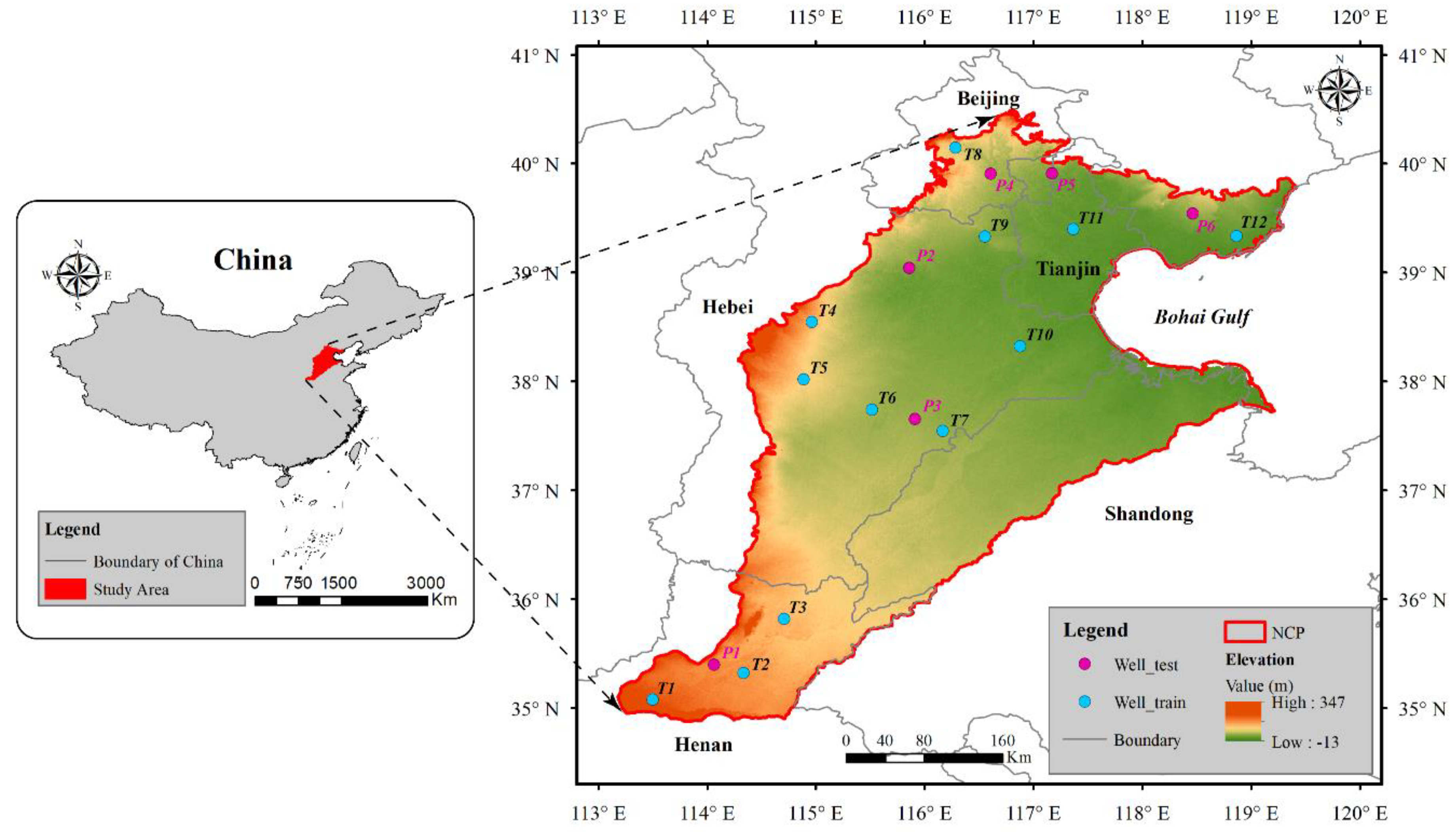
2.1. Study Area
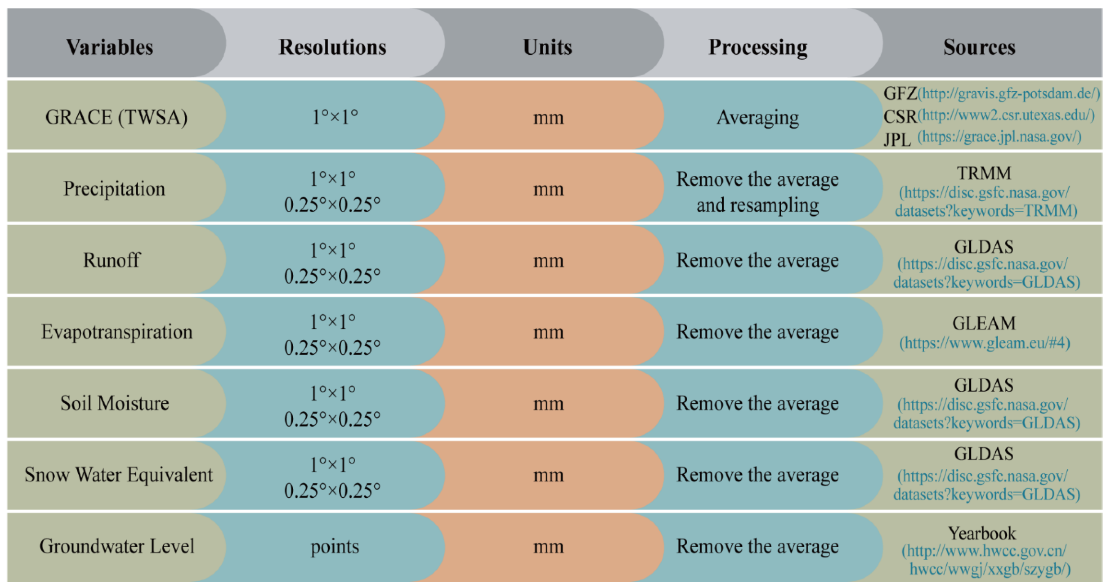
2.2. Data
2.2.1. GRACE TWSA
2.2.2. TRMM Precipitation
2.2.3. GLDAS Data
2.2.4. GLEAM Product
2.2.5. Groundwater Level
3. Methods
3.1. Gradient Boosting Decision Tree
3.2. Downscaling Approach Based on the Noah Model
3.3. Multiple Linear Regression
3.4. Fusion Model Design
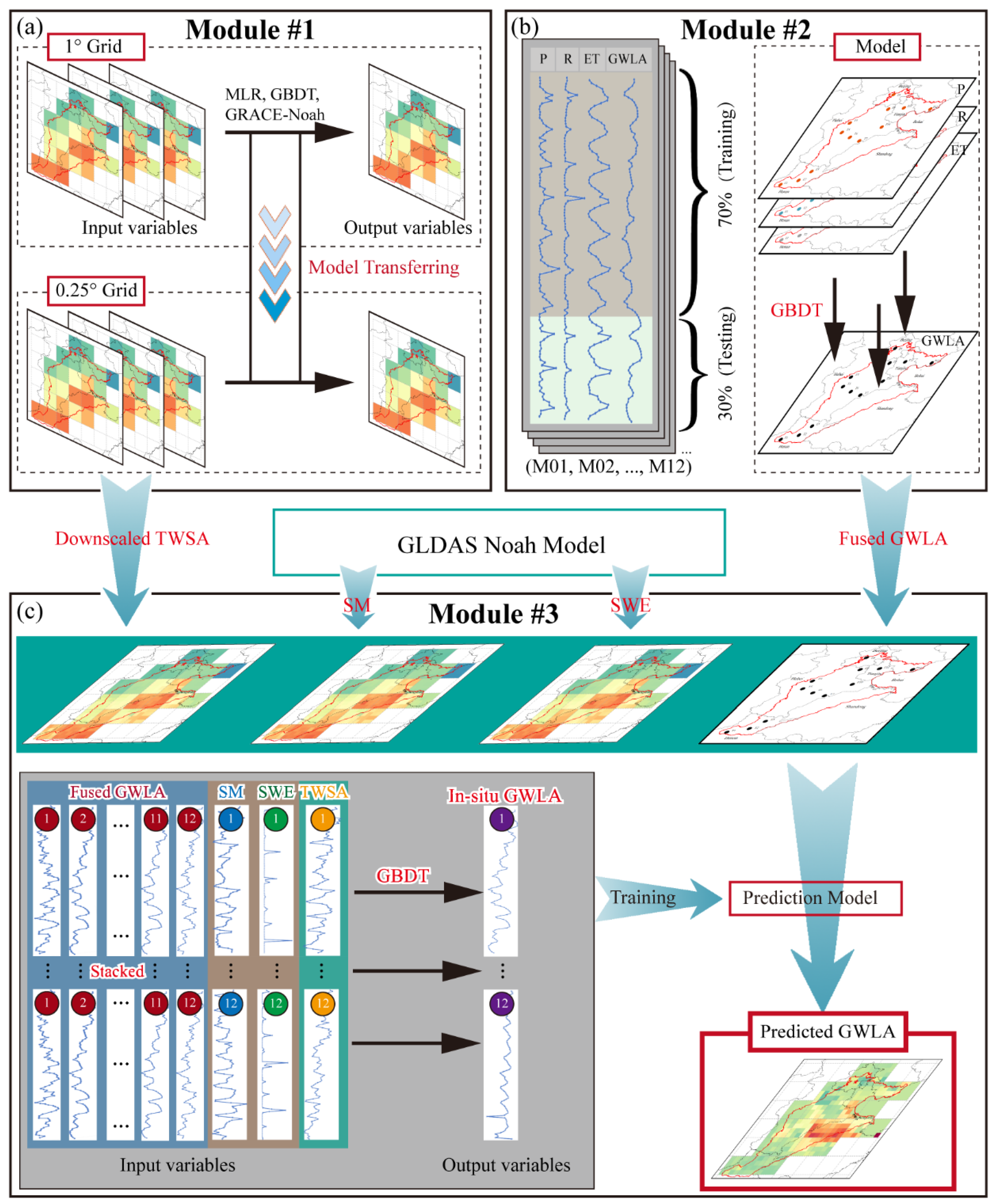
3.4.1. Module #1 for Downscaling
3.4.2. Module #2 for Data Fusion
3.4.3. Module #3 for Prediction
3.5. Model Evaluation and Data Analysis Standards
4. Results
4.1. Evaluation of Downscaling Models
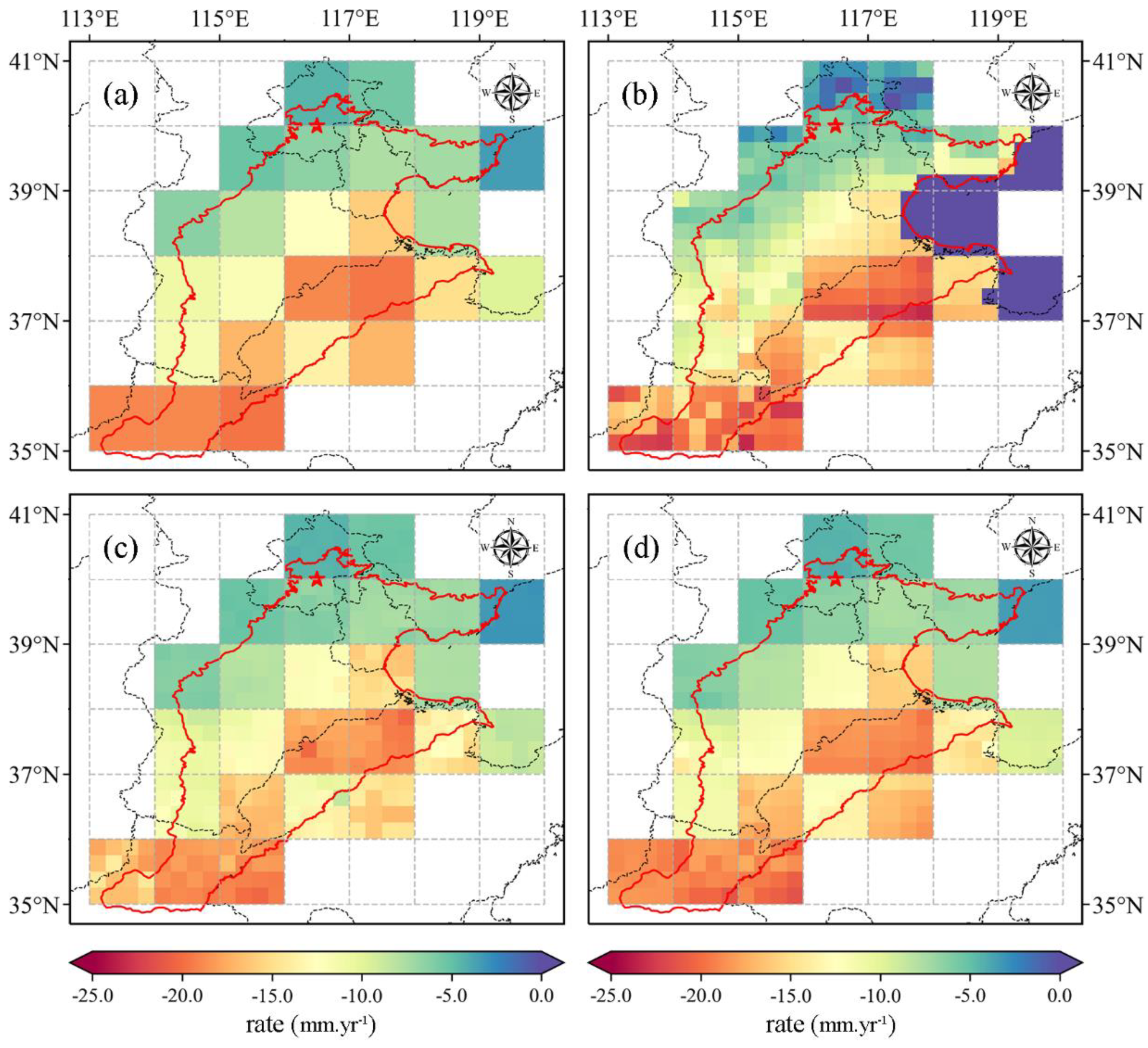
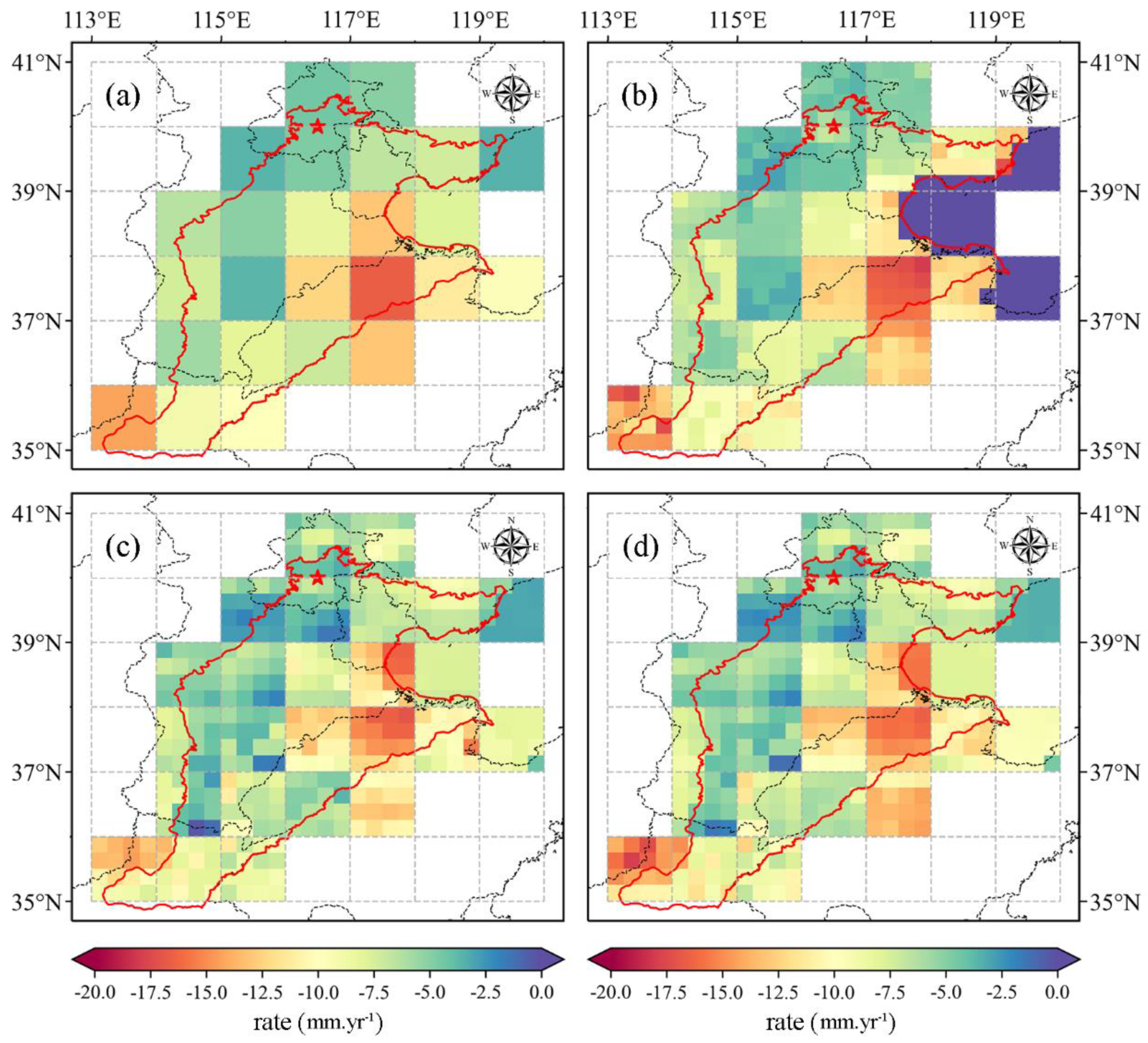
4.1.1. Spatial Resolution
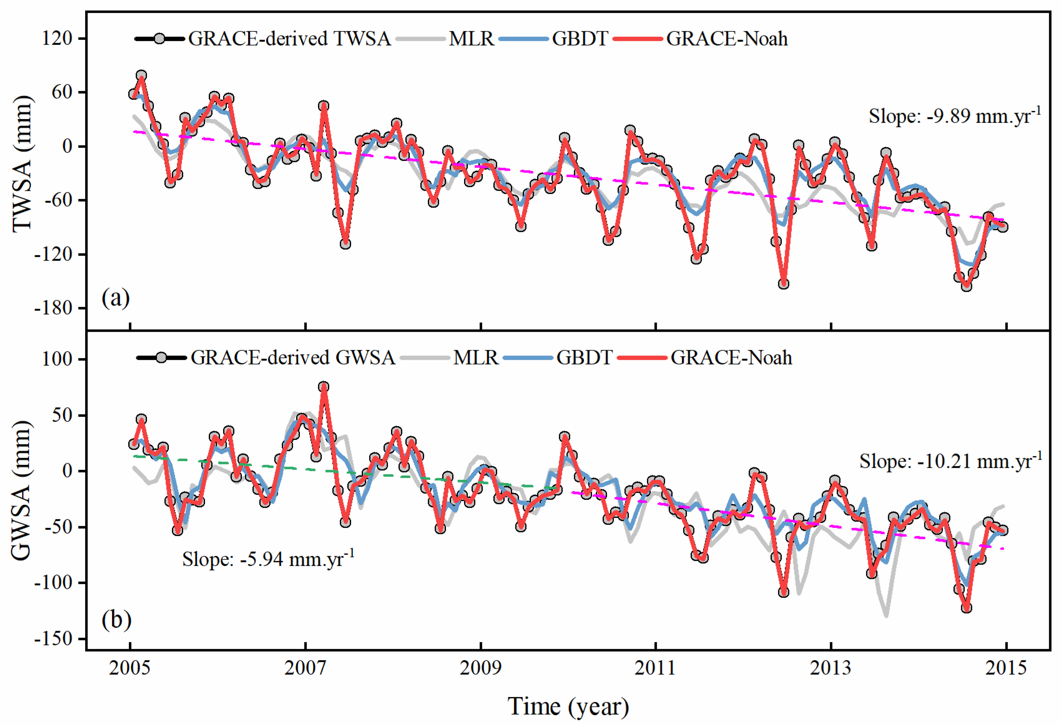
4.1.2. Temporal Resolution
4.2. Results of Data Fusion
4.3. Prediction Performance Analysis
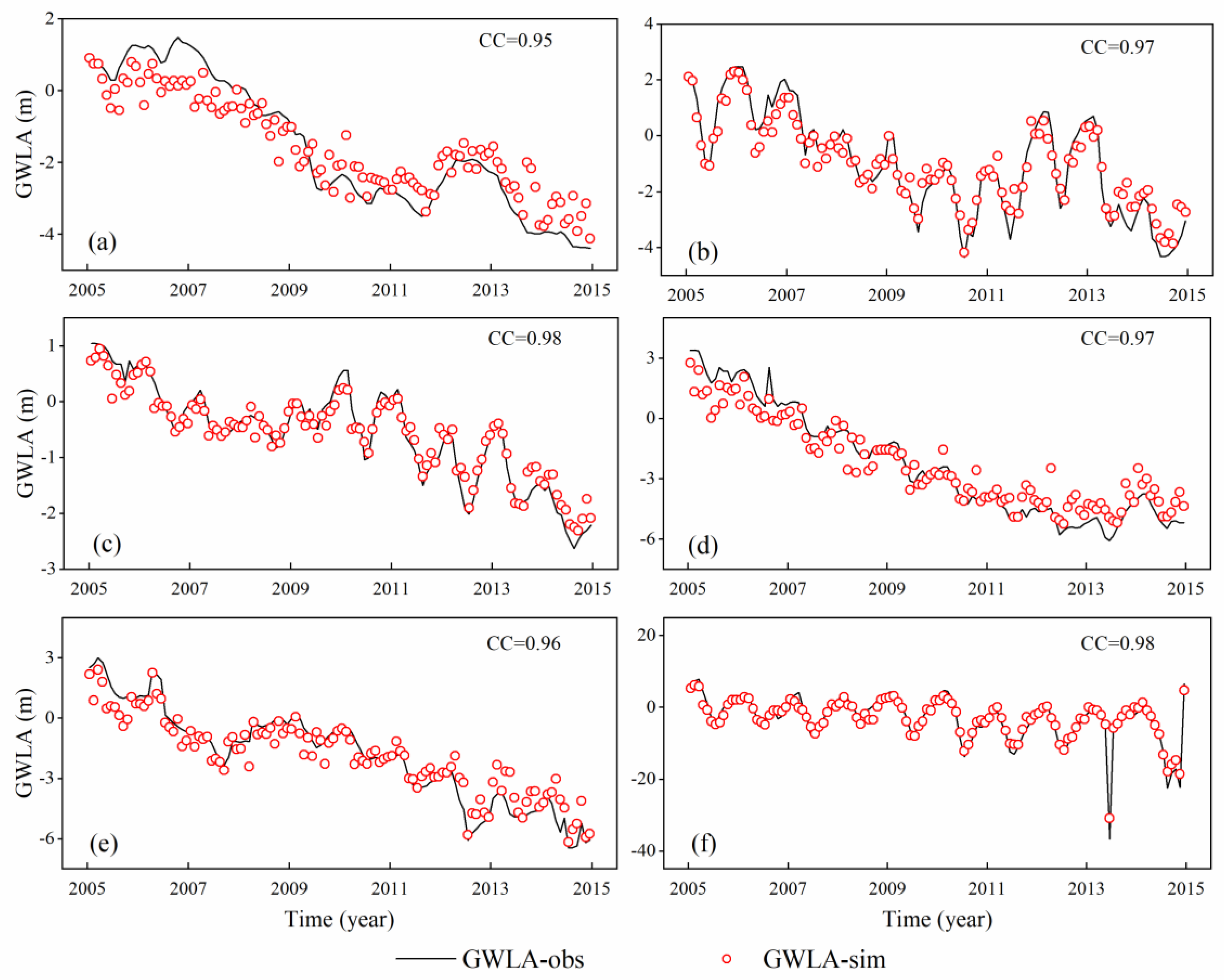
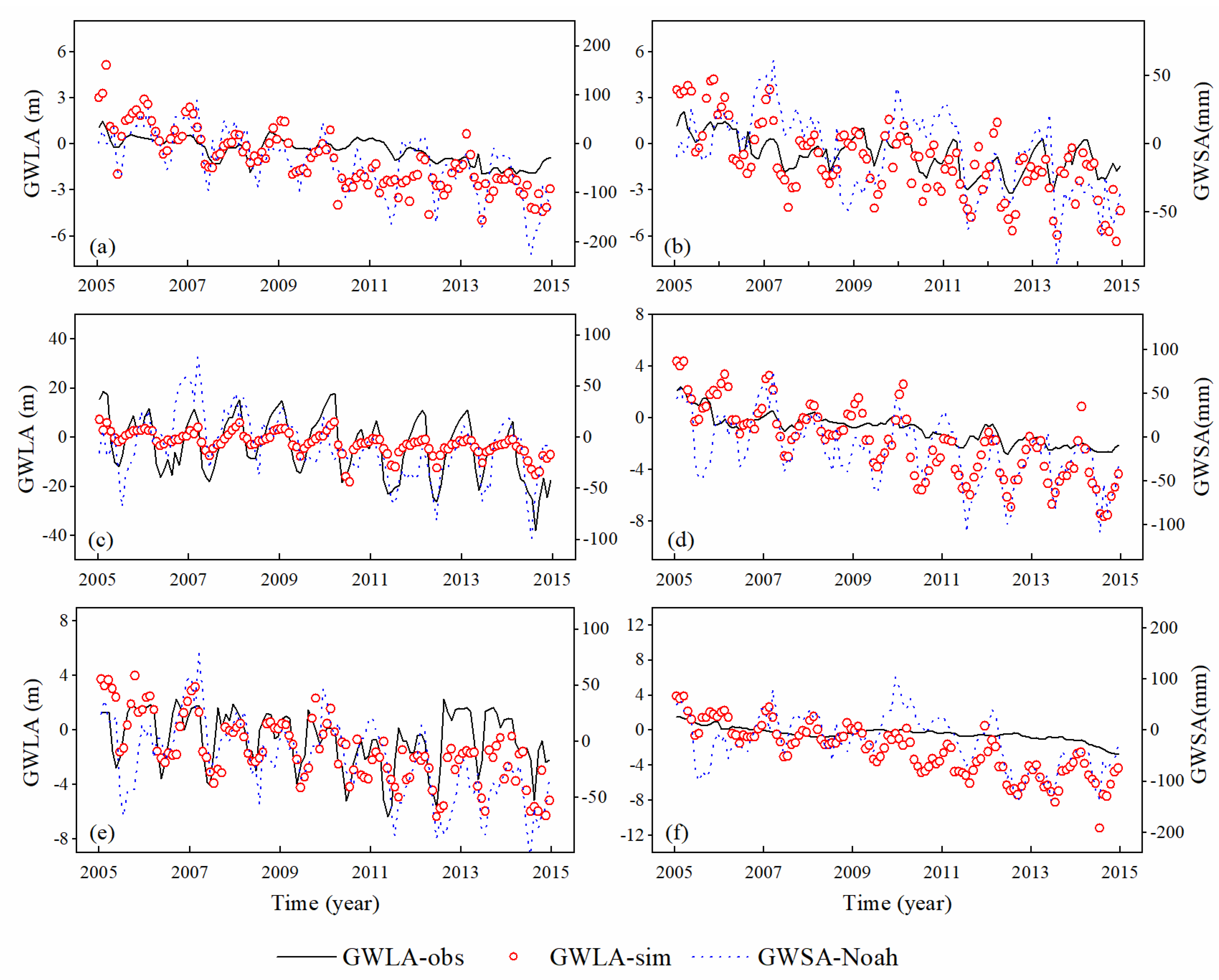
4.4. Verification of In-Situ Observations
5. Discussion
5.1. Efficacy of the Fusion Model
5.2. Limitations and Outlook
6. Conclusions
- (1)
- The machine learning-based fusion model, including three modules (downscaling module, data fusion module, and prediction module), is proposed in the NCP based on the empirical relationships between GRACE and climate drivers. These modules are both independent and integrated because the first two modules provide input variables for the prediction module while exhibiting their functions.
- (2)
- GRACE-derived TWSA is downscaled from 1° to 0.25° by utilizing three downscaling models (MLR, GBDT, and GRACE-Noah models). From the spatial resolution and temporal resolution, we compare the performances of downscaling models, and the findings indicate that the GRACE-Noah model performs the best performance, with the CC value of 0.99 and RMSE value of 1.49 mm in the whole study area. What is more, the verification results with in-situ observations of 18 wells also indicate the same result, with acceptable CC values ranging from 0.24 to 0.78.
- (3)
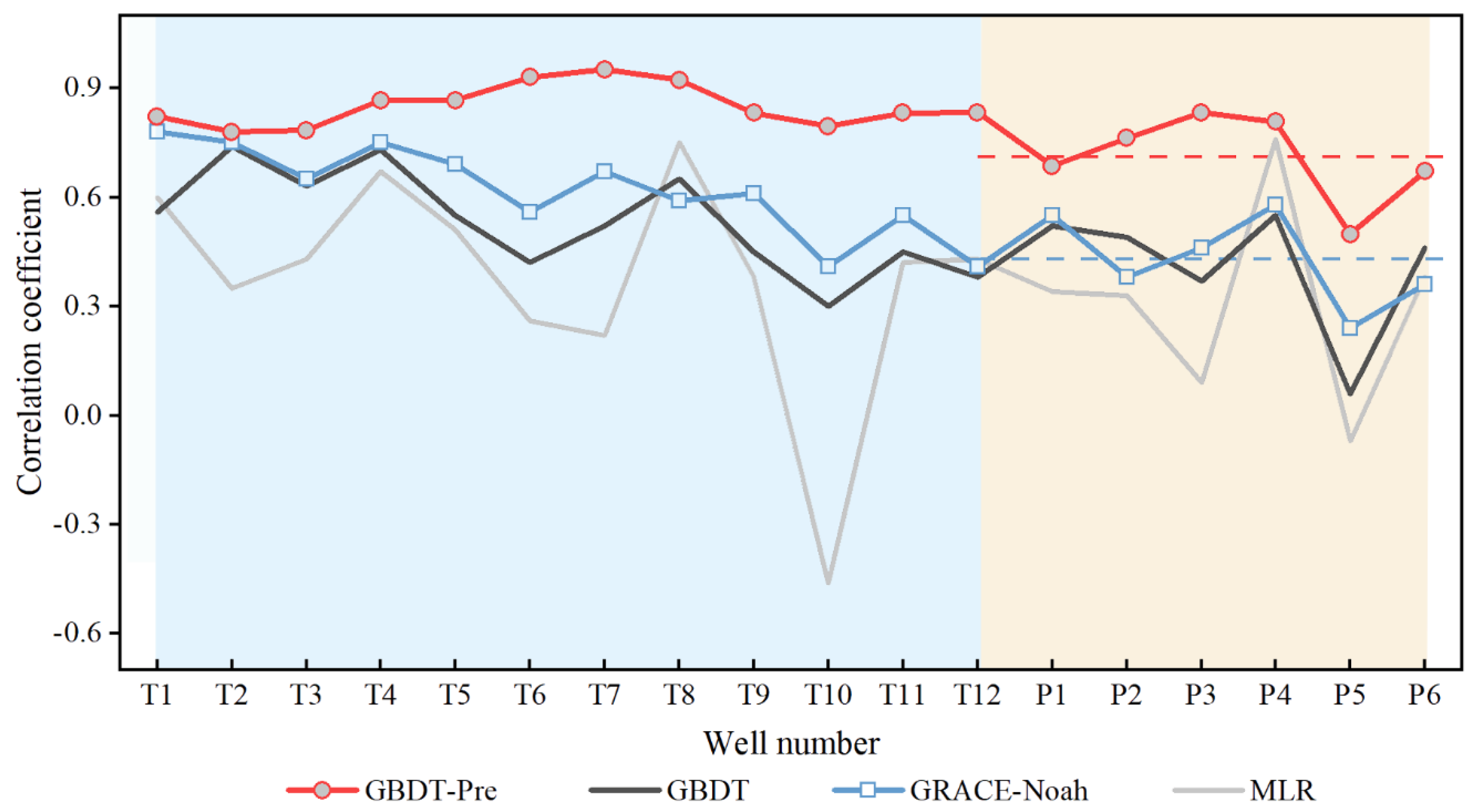
- Based on the downscaled and fused results, the prediction model is developed to obtain the GWLA within the whole NCP, and the verification results (CC values ranging from 0.50 to 0.95) indicate that the performance in simulating the long-term trend is ideal but may be insufficient in numerical prediction. Further, the average CC values of 6 test wells are calculated after prediction, which performs that the predicted result (0.71) is 65.12% higher than the downscaled result (0.43).
Author Contributions
Funding
Data Availability Statement
Conflicts of Interest
References
- Aeschbach-Hertig, W.; Gleeson, T. Regional strategies for the accelerating global problem of groundwater depletion. Nat. Geosci. 2012, 5, 853–861. [Google Scholar] [CrossRef]
- Gleeson, T.; Cuthbert, M.; Ferguson, G.; Perrone, D. Global groundwater sustainability, resources, and systems in the Anthropocene. Annu. Rev. Earth Planet. Sci. 2020, 48, 431–463. [Google Scholar] [CrossRef]
- Morris, B.L.; Lawrence, A.R.L.; Chilton, P.J.C.; Adams, B.; Calow, R.C.; Klinck, B.A. Groundwater and Its Susceptibility to Degradation: A Global Assessment of the Problem and Options for Management; UNEP Early Warning & Assessment Report Series RS. 03-3; UNEP: Nairobi, Kenya, 2003. [Google Scholar]
- Siebert, S.; Burke, J.; Faures, J.M.; Frenken, K.; Hoogeveen, J.; Döll, P.; Portmann, F.T. Groundwater use for irrigation—A global inventory. Hydrol. Earth Syst. Sci. 2010, 14, 1863–1880. [Google Scholar] [CrossRef]
- Taylor, R.G.; Scanlon, B.; Döll, P.; Rodell, M.; van Beek, R.; Wada, Y.; Longuevergne, L.; Leblanc, M.; Famiglietti, J.S.; Edmunds, M.; et al. Ground water and climate change. Nat. Clim. Chang. 2013, 3, 322–329. [Google Scholar] [CrossRef]
- Wu, W.; Lo, M.; Wada, Y.; Famiglietti, J.S.; Reager, J.T.; Yeh, P.J.F.; Ducharne, A.; Yang, Z. Divergent effects of climate change on future groundwater availability in key mid-latitude aquifers. Nat. Commun. 2020, 11, 3710. [Google Scholar] [CrossRef]
- Bierkens, M.F.P.; Wada, Y. Non-renewable groundwater use and groundwater depletion: A review. Environ. Res. Lett. 2019, 14, 063002. [Google Scholar] [CrossRef]
- Lall, U.; Josset, L.; Russo, T. A snapshot of the world’s groundwater challenges. Annu. Rev. Environ. Resour. 2020, 45, 1–24. [Google Scholar] [CrossRef]
- Yin, W.; Li, T.; Zheng, W.; Hu, L.; Han, S.; Tangdamrongsub, N.; Šprlák, M.; Huang, Z. Improving regional groundwater storage estimates from GRACE and global hydrological models over Tasmania, Australia. Hydrogeol. J. 2020, 28, 1809–1825. [Google Scholar] [CrossRef]
- Feng, W.; Shum, C.; Zhong, M.; Pan, Y. Groundwater storage changes in China from satellite gravity: An overview. Remote Sens. 2018, 10, 674. [Google Scholar] [CrossRef]
- Zhang, M.; Hu, L.; Yao, L.; Yin, W. Surrogate Models for Sub-Region Groundwater Management in the Beijing Plain, China. Water 2017, 9, 766. [Google Scholar] [CrossRef]
- Tapley, B.D.; Bettadpur, S.; Ries, J.C.; Thompson, P.F.; Watkins, M.M. GRACE measurements of mass variability in the earth system. Science 2004, 305, 503–505. [Google Scholar] [CrossRef] [PubMed]
- Tapley, B.D.; Bettadpur, S.; Watkins, M.; Reigber, C. The gravity recovery and climate experiment: Mission overview and early results. Geophys. Res. Lett. 2004, 31, L09607. [Google Scholar] [CrossRef]
- Swenson, S.; Wahr, J.; Milly, P.C.D. Estimated accuracies of regional water storage variations inferred from the Gravity Recovery and Climate Experiment (GRACE). Water Resour. Res. 2003, 39, W1223. [Google Scholar] [CrossRef]
- Zhong, Y.; Zhong, M.; Mao, Y.; Ji, B. Evaluation of Evapotranspiration for Exorheic Catchments of China during the GRACE Era: From a Water Balance Perspective. Remote Sens. 2020, 12, 511. [Google Scholar] [CrossRef]
- Yin, W.; Han, S.; Zheng, W.; Yeo, I.; Hu, L.; Tangdamrongsub, N.; Ghobadi-Far, K. Improved water storage estimates within the North China Plain by assimilating GRACE data into the CABLE model. J. Hydrol. 2020, 590, 125348. [Google Scholar] [CrossRef]
- Rodell, M.; Velicogna, I.; Famiglietti, J.S. Satellite-based estimates of groundwater depletion in India. Nature 2009, 460, 999–1002. [Google Scholar] [CrossRef]
- Yin, W.; Hu, L.; Jiao, J.J.; Lo Russo, S. Evaluation of groundwater storage variations in Northern China Using GRACE Data. Geofluids 2017, 2017, 8254824. [Google Scholar] [CrossRef]
- Famiglietti, J.S.; Rodell, M. Water in the balance. Science 2013, 340, 1300–1301. [Google Scholar] [CrossRef]
- Wilby, R.L.; Wigley, T.M.L. Downscaling general circulation model output: A review of methods and limitations. Prog. Phys. Geogr Earth Environ. 1997, 21, 530–548. [Google Scholar] [CrossRef]
- Tang, J.; Niu, X.; Wang, S.; Gao, H.; Wang, X.; Wu, J. Statistical downscaling and dynamical downscaling of regional climate in China: Present climate evaluations and future climate projections. J. Geophys. Res. Atmos. 2016, 121, 2110–2129. [Google Scholar] [CrossRef]
- Giorgi, F. Simulation of regional climate using a limited area model nested in a general circulation model. J. Clim. 1990, 3, 941–963. [Google Scholar] [CrossRef]
- Xu, Z.; Han, Y.; Yang, Z. Dynamical downscaling of regional climate: A review of methods and limitations. Sci. China Earth Sci. 2018, 62, 365–375. [Google Scholar] [CrossRef]
- Eicker, A.; Schumacher, M.; Kusche, J.; Döll, P.; Schmied, H.M. Calibration/Data assimilation approach for integrating GRACE data into the WaterGAP Global Hydrology Model (WGHM) using an Ensemble Kalman Filter: First results. Surv. Geophys. 2014, 35, 1285–1309. [Google Scholar] [CrossRef]
- Forootan, E.; Rietbroek, R.; Kusche, J.; Sharifi, M.A.; Awange, J.L.; Schmidt, M.; Omondi, P.; Famiglietti, J. Separation of large scale water storage patterns over Iran using GRACE, altimetry and hydrological data. Remote Sens. Environ. 2014, 140, 580–595. [Google Scholar] [CrossRef]
- Sahour, H.; Sultan, M.; Vazifedan, M.; Abdelmohsen, K.; Karki, S.; Yellich, J.A.; Gebremichael, E.; Alshehri, F.; Elbayoumi, T.M. Statistical applications to downscale GRACE-derived terrestrial water storage data and to fill temporal gaps. Remote Sens. 2020, 12, 533. [Google Scholar] [CrossRef]
- Nie, W.; Zaitchik, B.F.; Rodell, M.; Kumar, S.V.; Arsenault, K.R.; Li, B.; Getirana, A. Assimilating GRACE into a land surface model in the presence of an irrigation-induced groundwater trend. Water Resour. Res. 2019, 55, 11274–11294. [Google Scholar] [CrossRef]
- Khaki, M.; Schumacher, M.; Forootan, E.; Kuhn, M.; Awange, J.L.; van Dijk, A.I.J.M. Accounting for spatial correlation errors in the assimilation of GRACE into hydrological models through localization. Adv. Water Resour. 2017, 108, 99–112. [Google Scholar] [CrossRef]
- Wilby, R.L.; Wigley, T.M.L.; Conway, D.; Jones, P.D.; Hewitson, B.C.; Main, J.; Wilks, D.S. Statistical downscaling of general circulation model output: A comparison of methods. Water Resour. Res. 1998, 34, 2995–3008. [Google Scholar] [CrossRef]
- Gutiérrez, J.M.; San-Martín, D.; Brands, S.; Manzanas, R.; Herrera, S. Reassessing statistical downscaling techniques for their robust application under climate change conditions. J. Clim. 2013, 26, 171–188. [Google Scholar] [CrossRef]
- Ning, S.; Ishidaira, H.; Wang, J. Statistical downscaling of GRACE-derived terrestrial water storage using satellite and GLDAS products. J. Jpn. Soc. Civ. Eng. Ser. B1 Hydraul. Eng. 2014, 70, 133–138. [Google Scholar] [CrossRef]
- Wan, Z.; Zhang, K.; Xue, X.; Hong, Z.; Hong, Y.; Gourley, J.J. Water balance-based actual evapotranspiration reconstruction from ground and satellite observations over the conterminous United States. Water Resour. Res. 2015, 51, 6485–6499. [Google Scholar] [CrossRef]
- Yin, W.; Hu, L.; Zhang, M.; Wang, J.; Han, S. Statistical downscaling of GRACE-derived groundwater storage using ET data in the North China Plain. J. Geophys. Res. Atmos. 2018, 123, 5973–5987. [Google Scholar] [CrossRef]
- Miro, M.; Famiglietti, J. Downscaling GRACE remote sensing datasets to high-resolution groundwater storage change maps of California’s Central Valley. Remote Sens. 2018, 10, 143. [Google Scholar] [CrossRef]
- Kumar, P.S.; Praveen, T.V.; Prasad, M.A. Artificial neural network model for rainfall-runoff—A case study. Int. J. Hybrid Inf. Technol. 2016, 9, 263–272. [Google Scholar] [CrossRef]
- Seyoum, W.M.; Milewski, A.M. Improved methods for estimating local terrestrial water dynamics from GRACE in the Northern High Plains. Adv. Water Resour. 2017, 110, 279–290. [Google Scholar] [CrossRef]
- Chen, L.; He, Q.; Liu, K.; Li, J.; Jing, C. Downscaling of GRACE-derived groundwater storage based on the random forest model. Remote Sens. 2019, 11, 2979. [Google Scholar] [CrossRef]
- Rahaman, M.; Thakur, B.; Kalra, A.; Li, R.; Maheshwari, P. Estimating high-resolution groundwater storage from GRACE: A random forest approach. Environments 2019, 6, 63. [Google Scholar] [CrossRef]
- Fan, J.; Yue, W.; Wu, L.; Zhang, F.; Cai, H.; Wang, X.; Lu, X.; Xiang, Y. Evaluation of SVM, ELM and four tree-based ensemble models for predicting daily reference evapotranspiration using limited meteorological data in different climates of China. Agric. For. Meteorol. 2018, 263, 225–241. [Google Scholar] [CrossRef]
- Wu, Z.; Zhou, Y.; Wang, H. Real-Time Prediction of the Water Accumulation Process of Urban Stormy Accumulation Points Based on Deep Learning. IEEE Access 2020, 8, 151938–151951. [Google Scholar] [CrossRef]
- Wu, Z.; Zhou, Y.; Wang, H.; Jiang, Z. Depth prediction of urban flood under different rainfall return periods based on deep learning and data warehouse. Sci. Total Environ. 2020, 716, 137077. [Google Scholar] [CrossRef]
- Seyoum, W.; Kwon, D.; Milewski, A. Downscaling GRACE TWSA data into high-resolution groundwater level anomaly using machine learning-based models in a glacial aquifer system. Remote Sens. 2019, 11, 824. [Google Scholar] [CrossRef]
- Wang, S.; Shao, J.; Song, X.; Zhang, Y.; Huo, Z.; Zhou, X. Application of MODFLOW and geographic information system to groundwater flow simulation in North China Plain, China. Environ. Geol. 2008, 55, 1449–1462. [Google Scholar] [CrossRef]
- Liang, H.; Qin, W.; Hu, K.; Tao, H.; Li, B. Modelling groundwater level dynamics under different cropping systems and developing groundwater neutral systems in the North China Plain. Agric. Water Manag. 2019, 213, 732–741. [Google Scholar] [CrossRef]
- Gong, H.; Pan, Y.; Zheng, L.; Li, X.; Zhu, L.; Zhang, C.; Huang, Z.; Li, Z.; Wang, H.; Zhou, C. Long-term groundwater storage changes and land subsidence development in the North China Plain (1971–2015). Hydrogeol. J. 2018, 26, 1417–1427. [Google Scholar] [CrossRef]
- Zhang, C.; Duan, Q.; Yeh, P.J.F.; Pan, Y.; Gong, H.; Gong, W.; Di, Z.; Lei, X.; Liao, W.; Huang, Z.; et al. The effectiveness of the South-to-North Water Diversion Middle Route Project on water delivery and groundwater recovery in North China Plain. Water Resour. Res. 2020, e2019WR026759. [Google Scholar] [CrossRef]
- Shang, Q.; Liu, X.; Deng, X.; Zhang, B. Downscaling of GRACE datasets based on relevance vector machine using InSAR time series to generate maps of groundwater storage changes at local scale. J. Appl. Remote Sens. 2019, 13, 1–18. [Google Scholar] [CrossRef]
- Zheng, L.; Pan, Y.; Gong, H.; Huang, Z.; Zhang, C. Comparing Groundwater Storage Changes in Two Main Grain Producing Areas in China: Implications for Sustainable Agricultural Water Resources Management. Remote Sens. 2020, 12, 2151. [Google Scholar] [CrossRef]
- Wang, J.; Wang, E.; Yang, X.; Zhang, F.; Yin, H. Increased yield potential of wheat-maize cropping system in the North China Plain by climate change adaptation. Clim. Chang. 2012, 113, 825–840. [Google Scholar] [CrossRef]
- Guo, H.; Zhang, Z.; Cheng, G.; Li, W.; Li, T.; Jiao, J.J. Groundwater-derived land subsidence in the North China Plain. Environ. Earth Sci. 2015, 74, 1415–1427. [Google Scholar] [CrossRef]
- Liu, C.; Yu, J.; Eloise, K. Groundwater exploitation and its impact on the environment in the North China Plain. Water Int. 2001, 26, 265–272. [Google Scholar] [CrossRef]
- Feng, W.; Zhong, M.; Lemoine, J.; Biancale, R.; Hsu, H.; Xia, J. Evaluation of groundwater depletion in North China using the Gravity Recovery and Climate Experiment (GRACE) data and ground-based measurements. Water Resour. Res. 2013, 49, 2110–2118. [Google Scholar] [CrossRef]
- Sakura, Y.; Tang, C.; Yoshioka, R.; Ishiashi, H. Intensive Use of Groundwater in Some Areas of China and Japan. Intensive Use of Groundwater: Challenges and Opportunities; CRC Press: Boca Raton, FL, USA, 2003. [Google Scholar]
- Feng, W. GRAMAT: A comprehensive Matlab toolbox for estimating global mass variations from GRACE satellite data. Earth Sci. Inform. 2019, 12, 389–404. [Google Scholar] [CrossRef]
- Landerer, F.W.; Swenson, S.C. Accuracy of scaled GRACE terrestrial water storage estimates. Water Resour. Res. 2012, 48, W4531. [Google Scholar] [CrossRef]
- Monthly Mass Grids Land. Available online: https://grace.jpl.nasa.gov/data/get-data/monthly-mass-grids-land/ (accessed on 8 December 2020).
- Sakumura, C.; Bettadpur, S.; Bruinsma, S. Ensemble prediction and intercomparison analysis of GRACE time-variable gravity field models. Geophys. Res. Lett. 2014, 41, 1389–1397. [Google Scholar] [CrossRef]
- Kummerow, C.; Simpson, J.; Thiele, O.; Barnes, W.; Chang, A.T.C.; Stocker, E.; Adler, R.F.; Hou, A.; Kakar, R.; Wentz, F.; et al. The status of the Tropical Rainfall Measuring Mission (TRMM) after two years in Orbit. J. Appl. Meteorol. 2000, 39, 1965–1982. [Google Scholar] [CrossRef]
- NASA Dataset. Available online: https://disc.gsfc.nasa.gov/datasets?keywords=TRMM (accessed on 8 December 2020).
- Rodell, M.; Houser, P.R.; Jambor, U.; Gottschalck, J.; Mitchell, K.; Meng, C.J.; Arsenault, K.; Cosgrove, B.; Radakovich, J.; Bosilovich, M.; et al. The global land data assimilation system. B. Am. Meteorol. Soc. 2004, 85, 381–394. [Google Scholar] [CrossRef]
- Koster, R.D.; Suarez, M.J.; Heiser, M. Variance and Predictability of Precipitation at Seasonal-to-Interannual Timescales. J. Hydrometeorol. 2000, 1, 26–46. [Google Scholar] [CrossRef]
- Dai, Y.; Zeng, X.; Dickinson, R.E.; Baker, I.; Bonan, G.B.; Bosilovich, M.G.; Denning, A.S.; Dirmeyer, P.A.; Houser, P.R.; Niu, G.; et al. The Common Land Model. B. Am. Meteorol. Soc. 2003, 84, 1013–1024. [Google Scholar] [CrossRef]
- Chen, F.; Mitchell, K.; Schaake, J.; Xue, Y.; Pan, H.; Koren, V.; Duan, Q.Y.; Ek, M.; Betts, A. Modeling of land surface evaporation by four schemes and comparison with FIFE observations. J. Geophys. Res. Atmos. 1996, 101, 7251–7268. [Google Scholar] [CrossRef]
- Liang, X.; Lettenmaier, D.P.; Wood, E.F.; Burges, S.J. A simple hydrologically based model of land surface water and energy fluxes for general circulation models. J. Geophys. Res. 1994, 99, 14415–14428. [Google Scholar] [CrossRef]
- NASA Dataset. Available online: https://disc.gsfc.nasa.gov/datasets?keywords=GLDAS (accessed on 8 December 2020).
- Miralles, D.G.; Holmes, T.R.H.; De Jeu, R.A.M.; Gash, J.H.; Meesters, A.G.C.A.; Dolman, A.J. Global land-surface evaporation estimated from satellite-based observations. Hydrol. Earth Syst. Sci. 2011, 15, 453–469. [Google Scholar] [CrossRef]
- Martens, B.; Miralles, D.G.; Lievens, H.; van der Schalie, R.; de Jeu, R.A.M.; Fernández-Prieto, D.; Beck, H.E.; Dorigo, W.A.; Verhoest, N.E.C. GLEAM v3: Satellite-based land evaporation and root-zone soil moisture. Geosci. Model Dev. 2017, 10, 1903–1925. [Google Scholar] [CrossRef]
- Gleam Dataset. Available online: https://www.gleam.eu/#datasets (accessed on 8 December 2020).
- HWCC. Available online: http://www.hwcc.gov.cn/hwcc/wwgj/xxgb/szygb/ (accessed on 8 December 2020).
- Friedman, J.H. Greedy function approximation: A gradient boosting machine. Ann. Stat. 2001, 29, 1189–1232. [Google Scholar] [CrossRef]
- Rao, H.; Shi, X.; Rodrigue, A.K.; Feng, J.; Xia, Y.; Elhoseny, M.; Yuan, X.; Gu, L. Feature selection based on artificial bee colony and gradient boosting decision tree. Appl. Soft Comput. 2019, 74, 634–642. [Google Scholar] [CrossRef]
- Zhang, D.; Liu, X.; Bai, P. Assessment of hydrological drought and its recovery time for eight tributaries of the Yangtze River (China) based on downscaled GRACE data. J. Hydrol. 2019, 568, 592–603. [Google Scholar] [CrossRef]
- Aiken, L.S.; West, S.G.; Pitts, S.C.; Baraldi, A.N.; Wurpts, I.C. Multiple Linear Regression; Handbook of Psychology; American Cancer Society: Atlanta, GA, USA, 2012; pp. 511–542. [Google Scholar]
- Breiman, L.; Friedman, J.H. Predicting multivariate responses in multiple linear regression. J. R. Stat. Soc. Ser. B Stat. Methodol. 1997, 59, 3–54. [Google Scholar] [CrossRef]
- Chai, T.; Draxler, R.R. Root mean square error (RMSE) or mean absolute error (MAE)?—Arguments against avoiding RMSE in the literature. Geosci. Model Dev. 2014, 7, 1247–1250. [Google Scholar] [CrossRef]
- Nash, J.E.; Sutcliffe, J.V. River flow forecasting through conceptual models Part I—A discussion of principles. J. Hydrol. 1970, 10, 282–290. [Google Scholar] [CrossRef]
- McCuen, R.H.; Knight, Z.; Cutter, A.G. Evaluation of the Nash–Sutcliffe efficiency index. J. Hydrol. Eng. 2006, 11, 597–602. [Google Scholar] [CrossRef]
- Rodgers, J.L.; Nicewander, W.A. Thirteen ways to look at the correlation coefficient. Am. Stat. 1988, 42, 59–66. [Google Scholar] [CrossRef]
- Willmott, C.J.; Matsuura, K. Advantages of the mean absolute error (MAE) over the root mean square error (RMSE) in assessing average model performance. Clim. Res. 2005, 30, 79–82. [Google Scholar] [CrossRef]
- Oliver, M.A.; Webster, R. Kriging: A method of interpolation for geographical information systems. Int. J. Geogr. Inf. Syst. 1990, 4, 313–332. [Google Scholar] [CrossRef]
- Zhao, Q.; Zhang, B.; Yao, Y.; Wu, W.; Meng, G.; Chen, Q. Geodetic and hydrological measurements reveal the recent acceleration of groundwater depletion in North China Plain. J. Hydrol. 2019, 575, 1065–1072. [Google Scholar] [CrossRef]
- Huang, Z.; Pan, Y.; Gong, H.; Yeh, P.J.F.; Li, X.; Zhou, D.; Zhao, W. Subregional-scale groundwater depletion detected by GRACE for both shallow and deep aquifers in North China Plain. Geophys. Res. Lett. 2015, 42, 1791–1799. [Google Scholar] [CrossRef]


| Models | RMSE (mm) | MAE (mm) | NSE | CC | |
|---|---|---|---|---|---|
| TWSA | GRACE-Noah | 1.49 | 1.17 | 0.99 | 0.99 |
| GBDT | 18.00 | 10.20 | 0.85 | 0.93 | |
| MLR | 28.32 | 16.84 | 0.67 | 0.79 | |
| GWSA | GRACE-Noah | 1.24 | 0.81 | 0.99 | 0.99 |
| GBDT | 17.08 | 9.78 | 0.75 | 0.87 | |
| MLR | 27.23 | 15.81 | 0.36 | 0.68 |
| Model | Grid | RMSE (m) | MAE (m) | NSE | CC |
|---|---|---|---|---|---|
| M01 | T1 | 0.72 | 0.59 | 0.85 | 0.95 |
| M02 | T2 | 0.55 | 0.44 | 0.91 | 0.97 |
| M03 | T3 | 0.23 | 0.18 | 0.93 | 0.98 |
| M04 | T4 | 0.85 | 0.68 | 0.90 | 0.97 |
| M05 | T5 | 0.74 | 0.57 | 0.90 | 0.96 |
| M06 | T6 | 1.58 | 1.20 | 0.94 | 0.98 |
| M07 | T7 | 3.03 | 2.38 | 0.94 | 0.98 |
| M08 | T8 | 1.40 | 1.16 | 0.87 | 0.96 |
| M09 | T9 | 0.61 | 0.47 | 0.91 | 0.97 |
| M10 | T10 | 1.26 | 1.05 | 0.95 | 0.97 |
| M11 | T11 | 0.72 | 0.58 | 0.88 | 0.96 |
| M12 | T12 | 1.51 | 1.19 | 0.88 | 0.96 |
| Mean | 1.10 | 0.87 | 0.91 | 0.97 |
| Downscaled Results | Predicted Results | |||
|---|---|---|---|---|
| Wells | MLR | GBDT | GRACE-Noah | GBDT-Pre |
| T1 | 0.60 | 0.56 | 0.78 | 0.82 |
| T2 | 0.35 | 0.74 | 0.75 | 0.78 |
| T3 | 0.43 | 0.63 | 0.65 | 0.78 |
| T4 | 0.67 | 0.73 | 0.75 | 0.87 |
| T5 | 0.51 | 0.55 | 0.69 | 0.87 |
| T6 | 0.26 | 0.42 | 0.56 | 0.93 |
| T7 | 0.22 | 0.52 | 0.67 | 0.95 |
| T8 | 0.75 | 0.65 | 0.59 | 0.92 |
| T9 | 0.38 | 0.45 | 0.61 | 0.83 |
| T10 | −0.46 | 0.30 | 0.41 | 0.79 |
| T11 | 0.42 | 0.45 | 0.55 | 0.83 |
| T12 | 0.43 | 0.38 | 0.41 | 0.83 |
| P1 | 0.34 | 0.52 | 0.55 | 0.69 |
| P2 | 0.33 | 0.49 | 0.38 | 0.76 |
| P3 | 0.09 | 0.37 | 0.46 | 0.83 |
| P4 | 0.76 | 0.55 | 0.58 | 0.81 |
| P5 | −0.07 | 0.06 | 0.24 | 0.50 |
| P6 | 0.38 | 0.46 | 0.36 | 0.67 |
| Mean | 0.36 | 0.49 | 0.56 | 0.80 |
Publisher’s Note: MDPI stays neutral with regard to jurisdictional claims in published maps and institutional affiliations. |
© 2020 by the authors. Licensee MDPI, Basel, Switzerland. This article is an open access article distributed under the terms and conditions of the Creative Commons Attribution (CC BY) license (http://creativecommons.org/licenses/by/4.0/).
Share and Cite
Zhang, G.; Zheng, W.; Yin, W.; Lei, W. Improving the Resolution and Accuracy of Groundwater Level Anomalies Using the Machine Learning-Based Fusion Model in the North China Plain. Sensors 2021, 21, 46. https://doi.org/10.3390/s21010046
Zhang G, Zheng W, Yin W, Lei W. Improving the Resolution and Accuracy of Groundwater Level Anomalies Using the Machine Learning-Based Fusion Model in the North China Plain. Sensors. 2021; 21(1):46. https://doi.org/10.3390/s21010046
Chicago/Turabian StyleZhang, Gangqiang, Wei Zheng, Wenjie Yin, and Weiwei Lei. 2021. "Improving the Resolution and Accuracy of Groundwater Level Anomalies Using the Machine Learning-Based Fusion Model in the North China Plain" Sensors 21, no. 1: 46. https://doi.org/10.3390/s21010046
APA StyleZhang, G., Zheng, W., Yin, W., & Lei, W. (2021). Improving the Resolution and Accuracy of Groundwater Level Anomalies Using the Machine Learning-Based Fusion Model in the North China Plain. Sensors, 21(1), 46. https://doi.org/10.3390/s21010046