Sorting Objects from a Conveyor Belt Using POMDPs with Multiple-Object Observations and Information-Gain Rewards †

Abstract
:1. Introduction
2. Methodology
2.1. POMDP Model of the Sorting Task
- S is a set of states, taken discrete and finite for classical PODMPs. Individual states are denoted by .
- A is a set of actions available to the robot, again discrete and finite. Actions are .
- is a stochastic state transition function. Each function value gives the probability that the next state is after executing action a in current state s.
- is a reward function, where is the reward obtained by executing a in s. Note that sometimes rewards may also depend on the next state; in that case, is the expectation taken over the value of the next state. Moreover, rewards are classically assumed to be bounded.
- Z is a set of observations, discrete and finite. The robot does not have access to the underlying state s. Instead, it observes the state through imperfect sensors, which read an observation at each step.
- is a stochastic observation function, which defines how observations are seen as a function of the underlying states and actions. Specifically, is the probability of observing value z when reaching state after executing action a.
- is a discount factor.
- Motion state , meaning simply the viewpoint of the robot. There are K such viewpoints.
- Motion action , meaning the choice of next viewpoint.
- Motion transition function:which simply says that the robot always moves deterministically to the chosen viewpoint.
2.2. Adding Rewards Based on the Information Gain
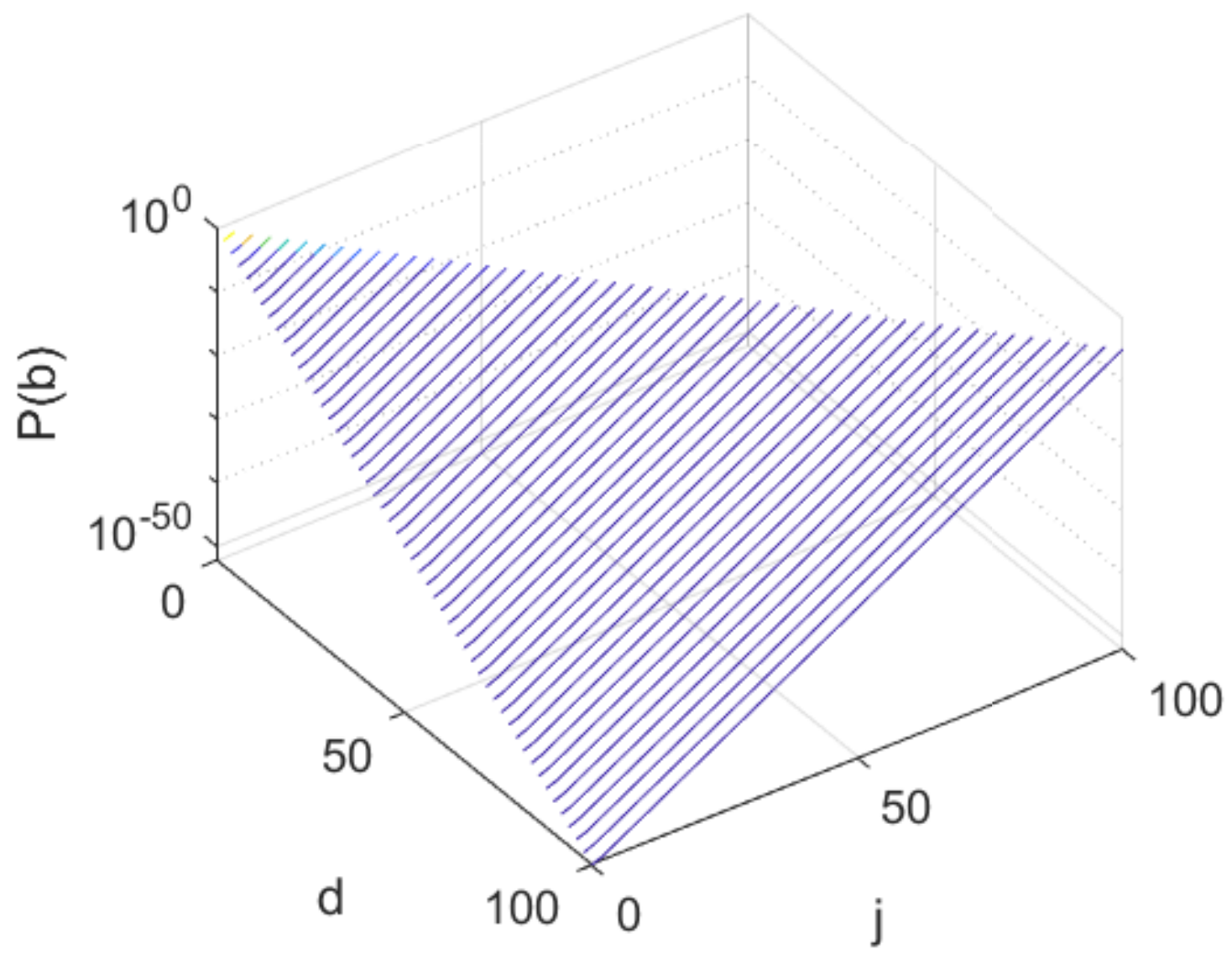
2.3. Complexity Insight
2.4. Hardware, Software, and Experimental Setup
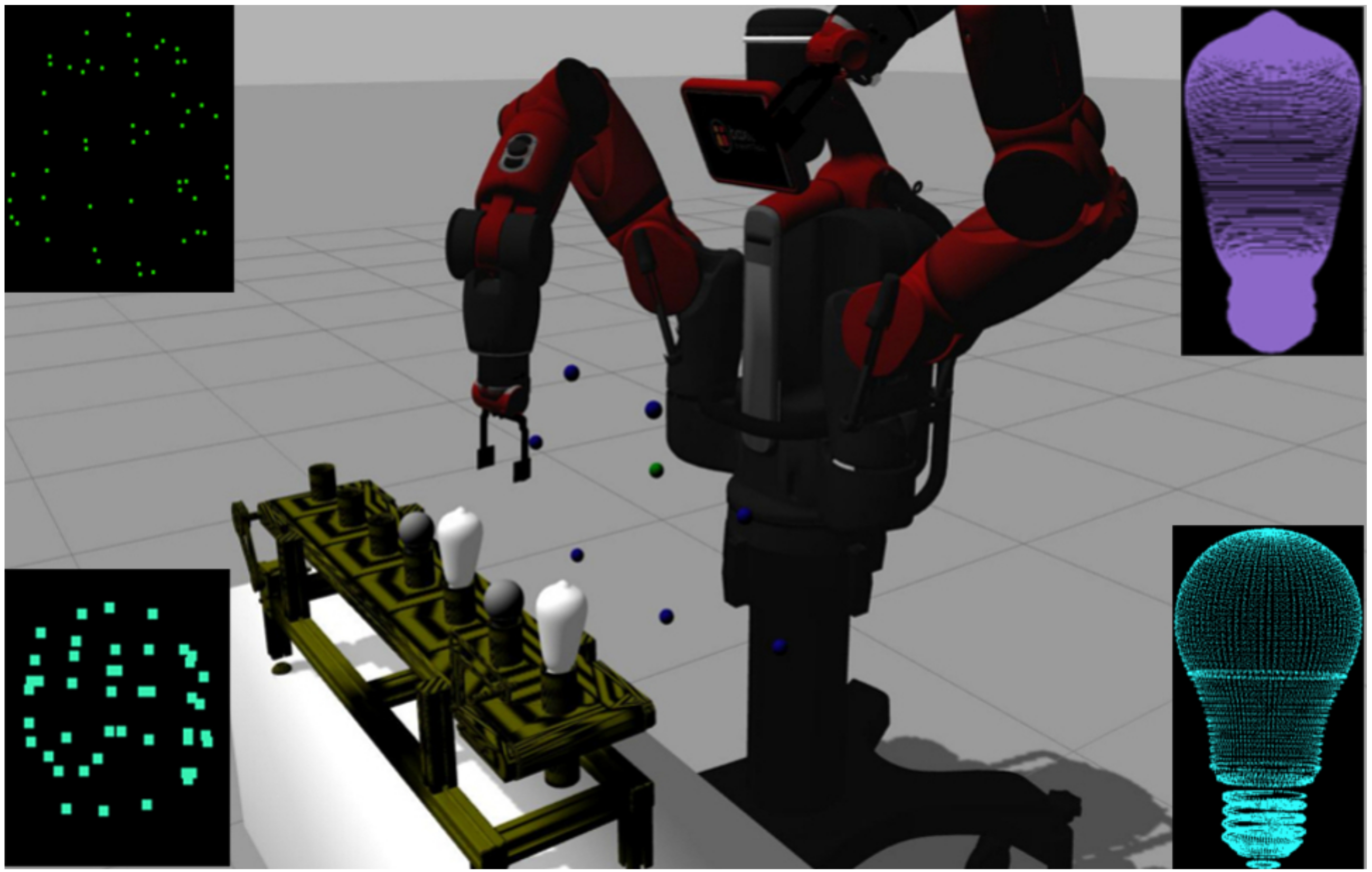
2.4.1. Hardware and Software Base
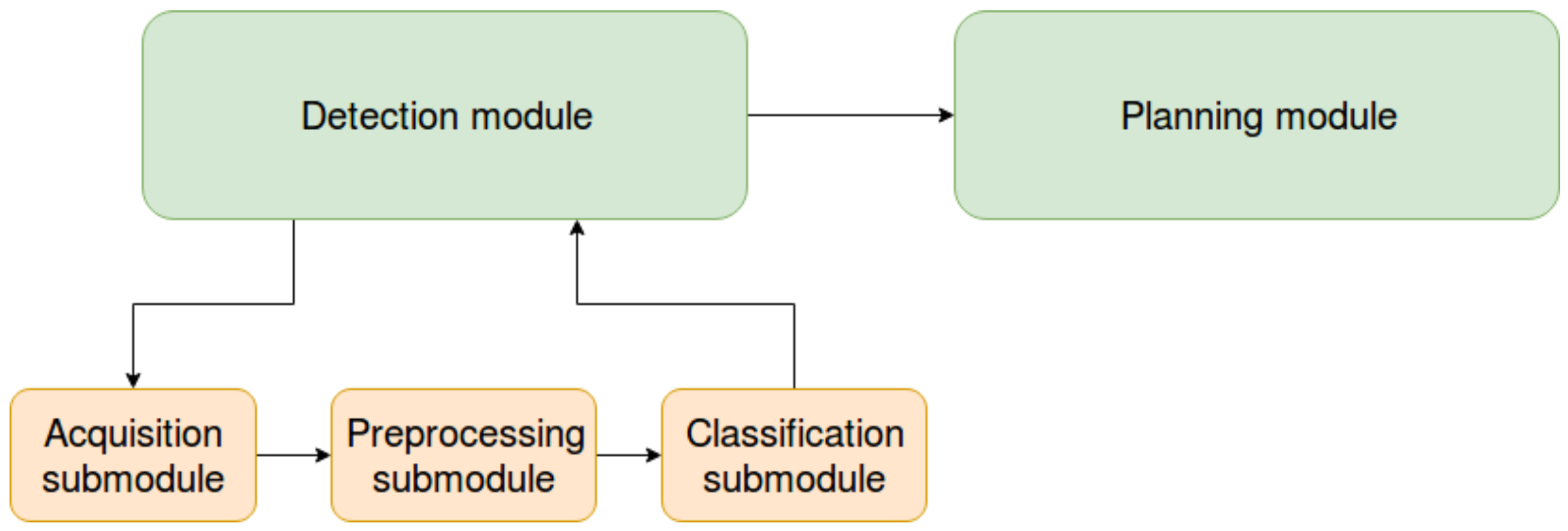
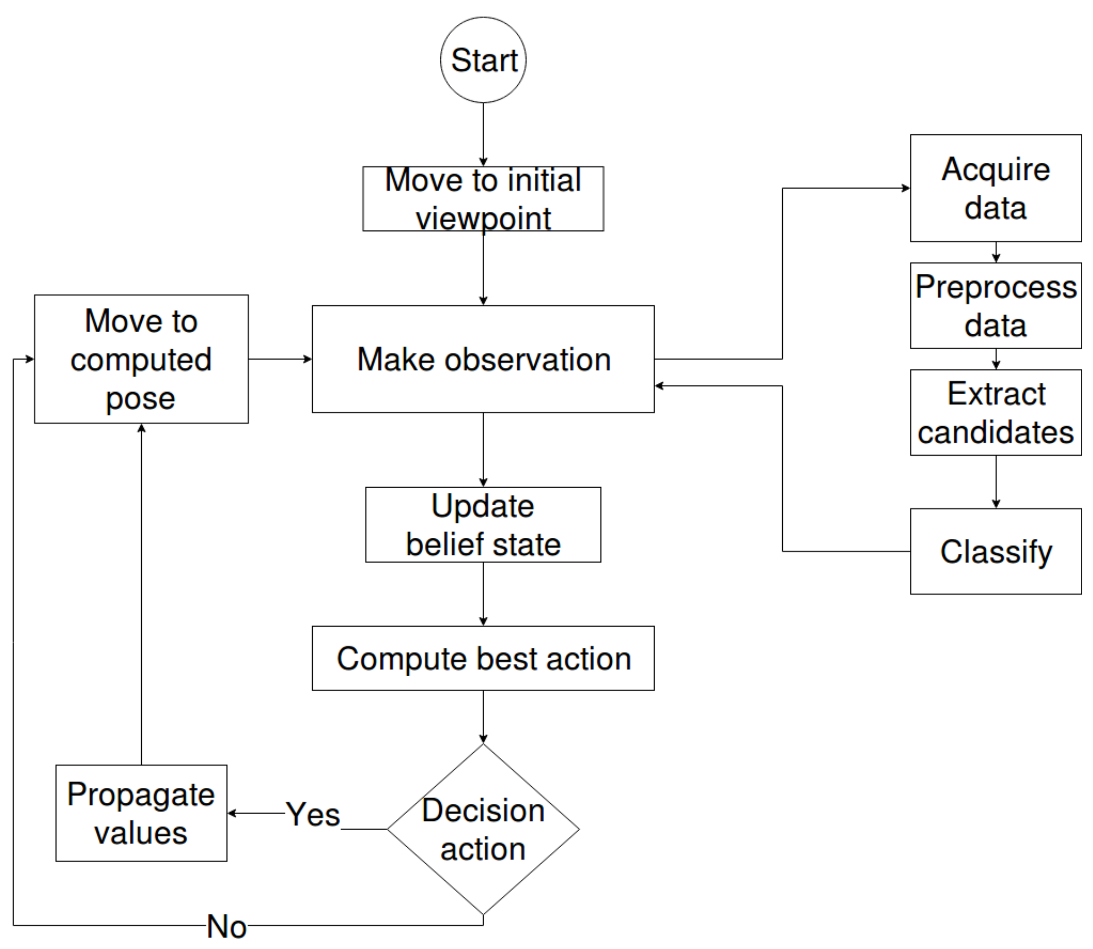
2.4.2. Active Perception Pipeline
2.4.3. Workflow
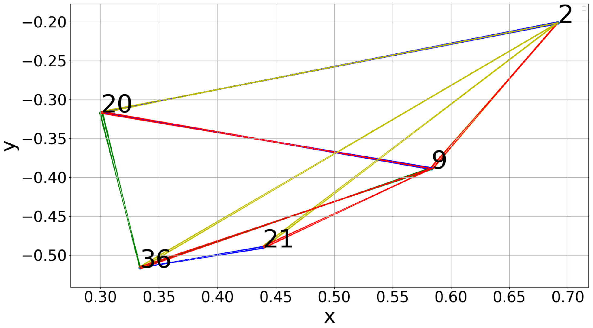
2.4.4. Experimental Setup
3. Results and Discussion
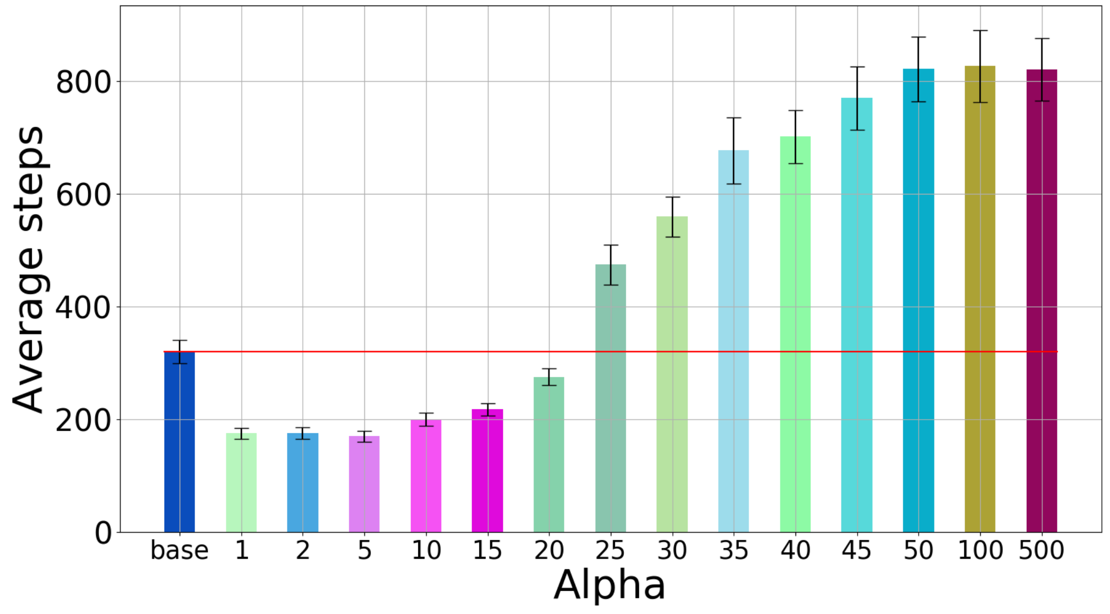
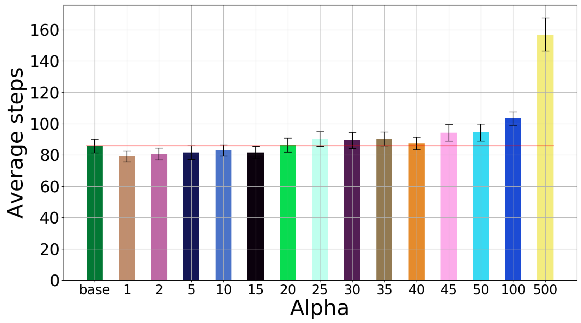
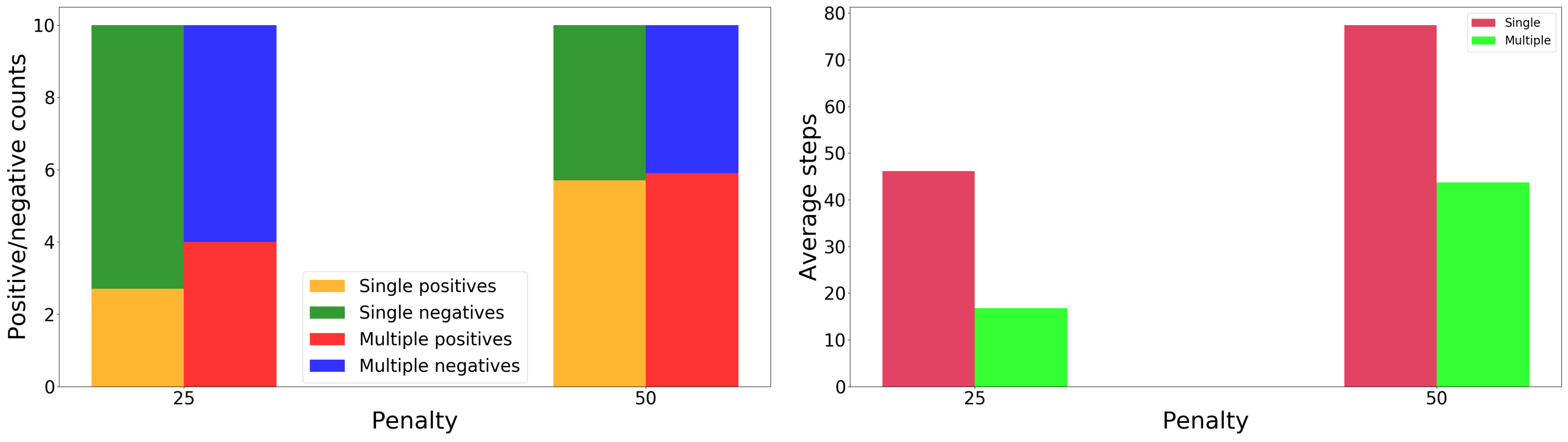
3.1. Effect of Decision Penalty and Multiple-Position Observations
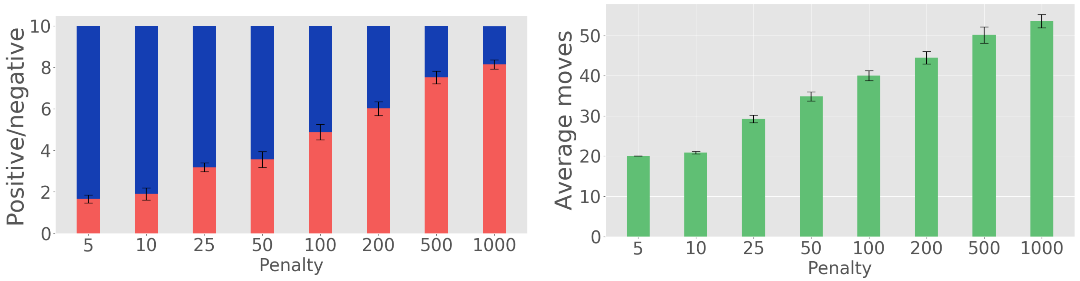
3.1.1. Single-Position Observations. Comparison to Baseline
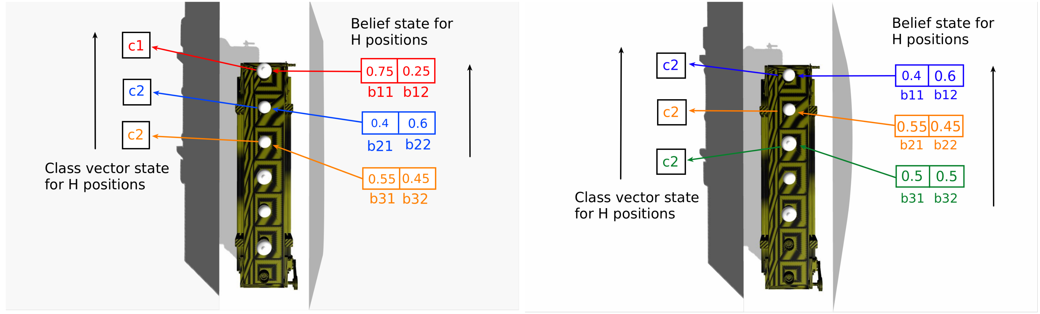
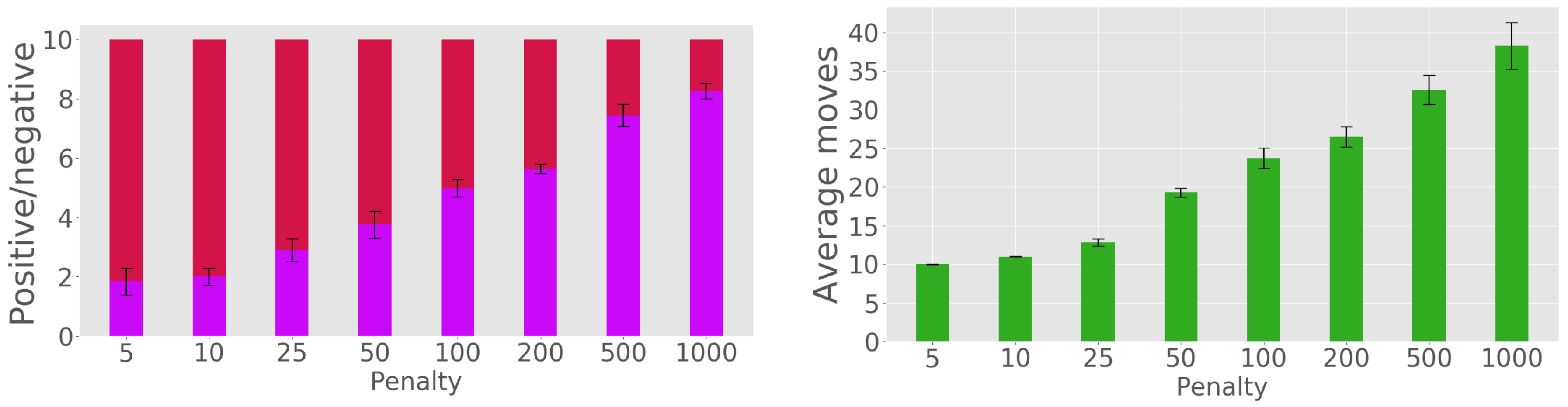
3.1.2. Two-Position Observations
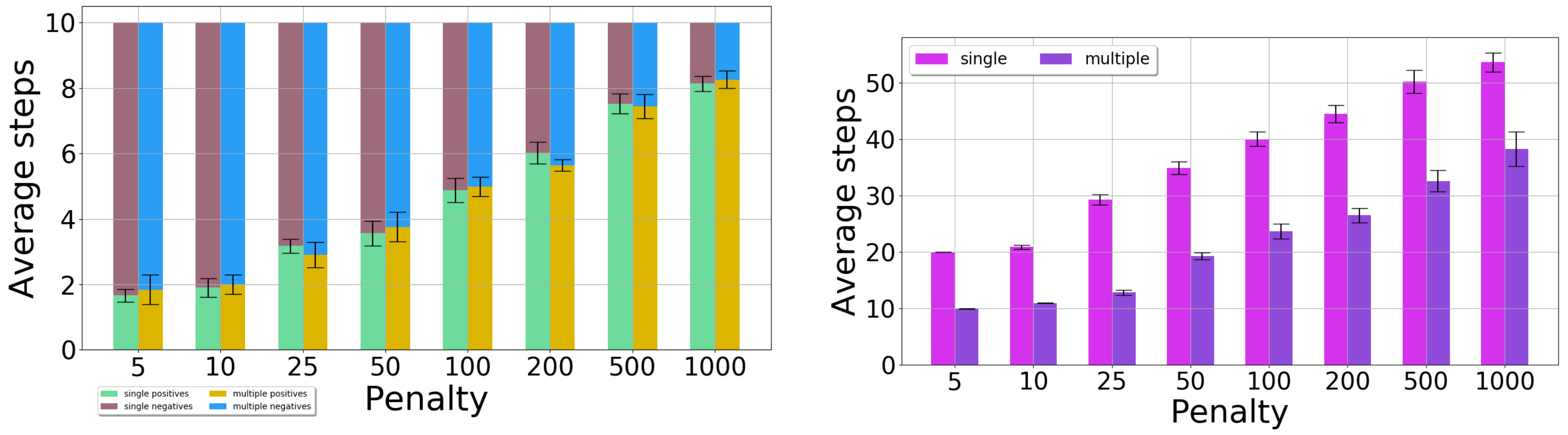
3.1.3. Single-Position Versus Two-Position Observations
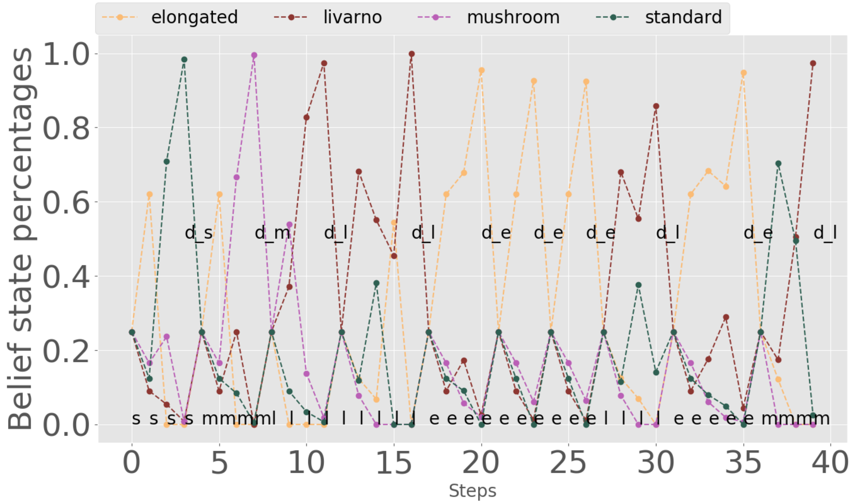
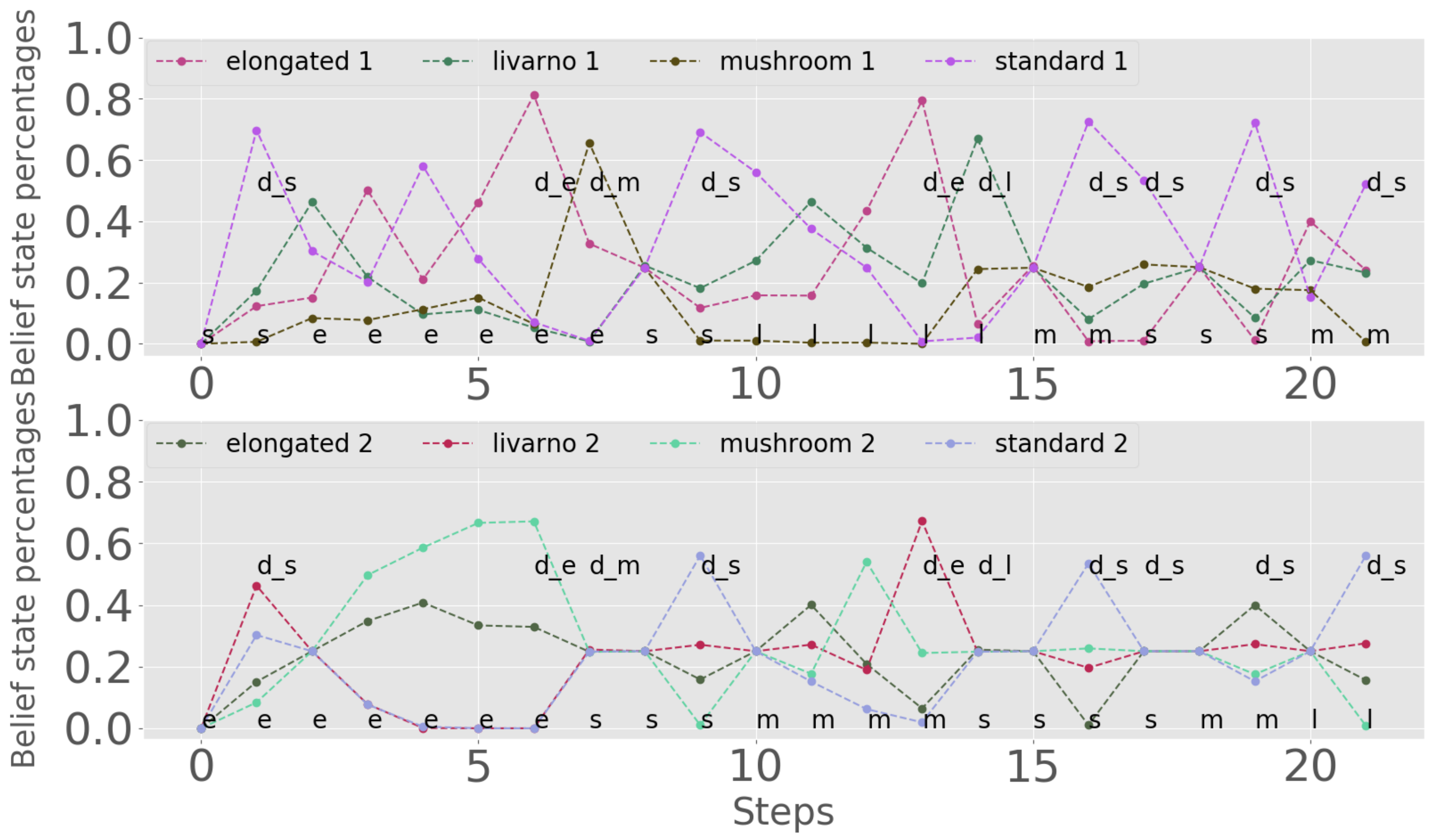
3.2. Effect of Including the Information Gain
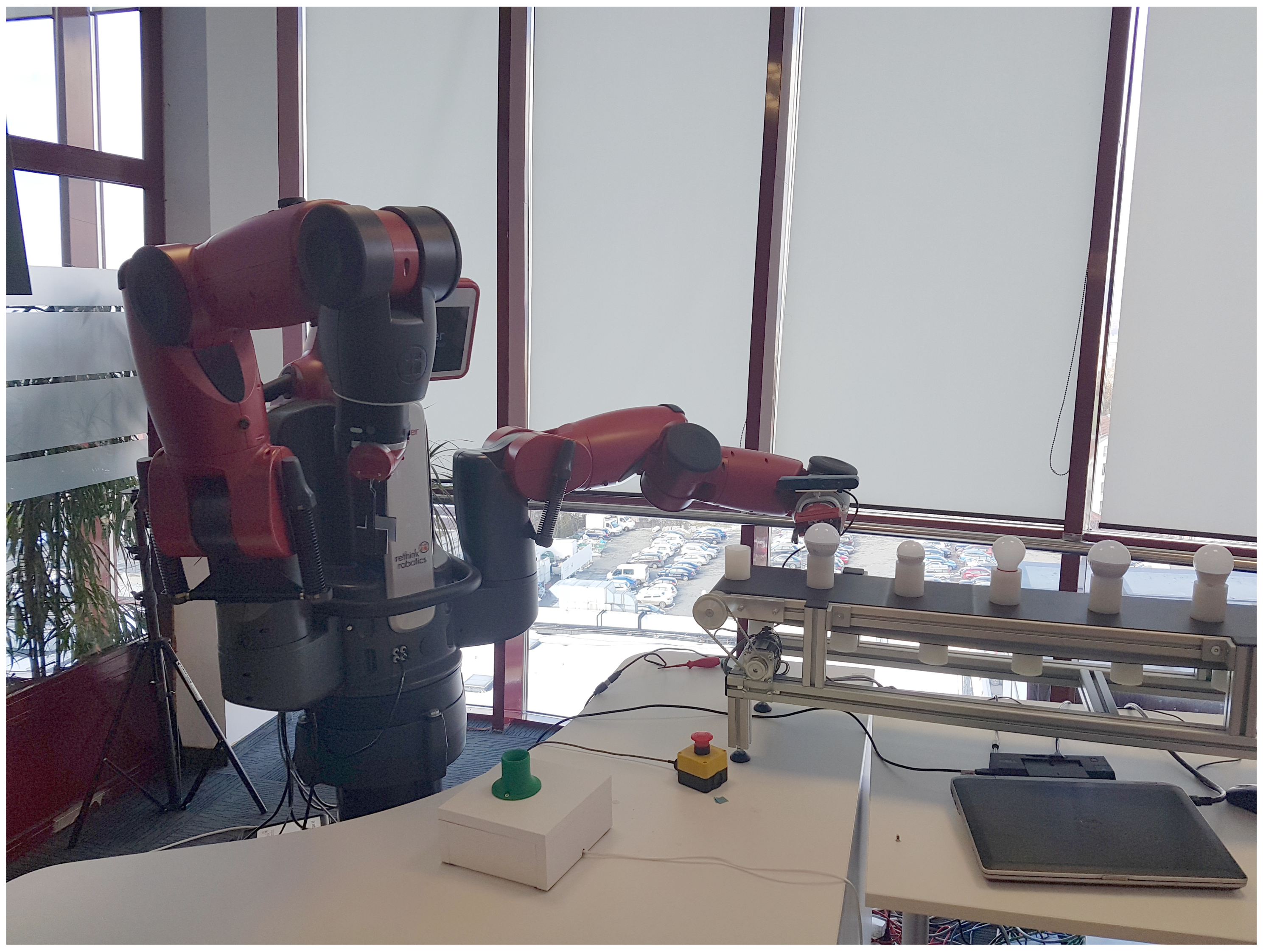
3.3. Real-Robot Experiments
4. Conclusions
Author Contributions
Funding
Conflicts of Interest
Abbreviations
| DESPOT | Determinized Sparse Partially Observable Tree |
| PCL | Point Cloud Library |
| POMDP | Partially Observable Markov Decision Process |
| RGB-D | Red-Green-Blue-Depth |
| ROS | Robot Operating System |
| VFH | Viewpoing Feature Histogram |
References
- Militaru, C.; Mezei, A.D.; Tamas, L. Object handling in cluttered indoor environment with a mobile manipulator. In Proceedings of the 2016 IEEE International Conference on Automation, Quality and Testing, Robotics (AQTR), Cluj-Napoca, Romania, 19–21 May 2016; pp. 1–6. [Google Scholar]
- Militaru, C.; Mezei, A.D.; Tamas, L. Lessons Learned from a Cobot Integration into MES. In Proceedings of the ICRA—Recent Advances in Dynamics for Industrial Applications Workshop, Singapore, 24–28 May 2017. [Google Scholar]
- Militaru, C.; Mezei, A.D.; Tamas, L. Industry 4.0 – MES Vertical Integration Use-case with a Cobot. In Proceedings of the ICRA—Recent Advances in Dynamics for Industrial Applications Workshop, Singapore, 24–28 May 2017. [Google Scholar]
- Páll, E.; Tamás, L.; Buşoniu, L. Analysis and a home assistance application of online AEMS2 planning. In Proceedings of the 2016 IEEE/RSJ International Conference on Intelligent Robots and Systems (IROS), Daejeon, Korea, 9–14 October 2016; pp. 5013–5019. [Google Scholar]
- Bajcsy, R. Active perception. Proc. IEEE 1988, 76, 966–1005. [Google Scholar] [CrossRef]
- Aloimonos, J.; Weiss, I.; Bandopadhay, A. Active vision. Int. J. Comput. Vis. 1988, 1, 333–356. [Google Scholar] [CrossRef]
- Eidenberger, R.; Scharinger, J. Active perception and scene modeling by planning with probabilistic 6d object poses. In Proceedings of the 2010 IEEE/RSJ International Conference on Intelligent Robots and Systems, Taipei, Taiwan, 18–22 October 2010; pp. 1036–1043. [Google Scholar]
- Velez, J.; Hemann, G.; Huang, A.S.; Posner, I.; Roy, N. Planning to perceive: Exploiting mobility for robust object detection. In Proceedings of the Twenty-First International Conference on Automated Planning and Scheduling, Freiburg, Germany, 11–16 June 2011. [Google Scholar]
- Holz, D.; Nieuwenhuisen, M.; Droeschel, D.; Stückler, J.; Berner, A.; Li, J.; Klein, R.; Behnke, S. Active recognition and manipulation for mobile robot bin picking. In Gearing Up and Accelerating Cross-fertilization between Academic and Industrial Robotics Research in Europe; Springer: Berlin/Heidelberg, Germany, 2014; pp. 133–153. [Google Scholar]
- Patten, T.; Zillich, M.; Fitch, R.; Vincze, M.; Sukkarieh, S. Viewpoint Evaluation for Online 3-D Active Object Classification. IEEE Robot. Autom. Lett. 2016, 1, 73–81. [Google Scholar] [CrossRef]
- Atanasov, N.; Le Ny, J.; Daniilidis, K.; Pappas, G.J. Decentralized active information acquisition: Theory and application to multi-robot SLAM. In Proceedings of the 2015 IEEE International Conference on Robotics and Automation (ICRA), Seattle, WA, USA, 26–30 May 2015; pp. 4775–4782. [Google Scholar]
- Aleotti, J.; Lodi Rizzini, D.; Caselli, S. Perception and Grasping of Object Parts from Active Robot Exploration. J. Intell. Robot. Syst. Theory Appl. 2014, 76, 401–425. [Google Scholar] [CrossRef]
- Cowley, A.; Cohen, B.; Marshall, W.; Taylor, C.; Likhachev, M. Perception and motion planning for pick-and-place of dynamic objects. In Proceedings of the IEEE/RSJ International Conference on Intelligent Robots and Systems (IROS 2013), Tokyo, Japan, 3–7 November 2013; pp. 816–823. [Google Scholar]
- Atanasov, N.; Sankaran, B.; Le Ny, J.; Pappas, G.J.; Daniilidis, K. Nonmyopic view planning for active object classification and pose estimation. IEEE Trans. Robot. 2014, 30, 1078–1090. [Google Scholar] [CrossRef]
- Somani, A.; Ye, N.; Hsu, D.; Lee, W.S. DESPOT: Online POMDP Planning with Regularization. In Proceedings of the Advances in Neural Information Processing Systems, Lake Tahoe, NV, USA, 5–10 December 2013; pp. 1772–1780. [Google Scholar]
- Spaan, M.T.; Veiga, T.S.; Lima, P.U. Decision-theoretic planning under uncertainty with information rewards for active cooperative perception. Auton. Agents Multi-Agent Syst. 2014, 29, 1–29. [Google Scholar] [CrossRef]
- Spaan, M.T.J.; Veiga, T.S.; Lima, P.U. Active Cooperative Perception in Network Robot Systems Using POMDPs. In Proceedings of the International Conference on Intelligent Robots and Systems (IROS), Taipei, Taiwan, 18–22 October 2010; pp. 4800–4805. [Google Scholar]
- Mafi, N.; Abtahi, F.; Fasel, I. Information theoretic reward shaping for curiosity driven learning in POMDPs. In Proceedings of the 2011 IEEE International Conference on Development and Learning (ICDL), Frankfurt am Main, Germany, 24–27 August 2011; Volume 2, pp. 1–7. [Google Scholar]
- Mezei, A.; Tamás, L.; Busoniu, L. Sorting objects from a conveyor belt using active perception with a POMDP model. In Proceedings of the 18th European Control Conference, Naples, Italy, 25–28 June 2019; pp. 2466–2471. [Google Scholar]
- Ross, S.; Pineau, J.; Paquet, S.; Chaib-draa, B. Online Planning Algorithms for POMDPs. J. Artif. Int. Res. 2008, 32, 663–704. [Google Scholar] [CrossRef]
- Ross, S.; Chaib-draa, B. AEMS: An Anytime Online Search Algorithm for Approximate Policy Refinement in Large POMDPs. In Proceedings of the 20th International Joint Conference on Artificial Intelligence (IJCAI-07), Hyderabad, India, 6–12 January 2007. [Google Scholar]
- Zhang, Z.; Littman, M.; Chen, X. Covering number as a complexity measure for POMDP planning and learning. In Proceedings of the Twenty-Sixth AAAI Conference on Artificial Intelligence, Toronto, ON, Canada, 22–26 July 2012. [Google Scholar]
- Zhang, Z.; Hsu, D.; Lee, W.S. Covering Number for Efficient Heuristic-based POMDP Planning. In Proceedings of the 31th International Conference on Machine Learning, Beijing, China, 21–26 June 2014; pp. 28–36. [Google Scholar]
- Mezei, A.; Tamas, L. Active perception for object manipulation. In Proceedings of the IEEE 12th International Conference on Intelligent Computer Communication and Processing, Cluj-Napoca, Romania, 8–10 September 2016; pp. 269–274. [Google Scholar]
- Rusu, R.B.; Cousins, S. 3D is here: Point Cloud Library (PCL). In Proceedings of the 2011 IEEE International Conference on Robotics and Automation, Shanghai, China, 9–13 May 2011; pp. 1–4. [Google Scholar]
- Tamas, L.; Jensen, B. Robustness analysis of 3d feature descriptors for object recognition using a time-of-flight camera. In Proceedings of the 22nd Mediterranean Conference on Control and Automation, Palermo, Italy, 16–19 June 2014; pp. 1020–1025. [Google Scholar]
- Rusu, R.B.; Bradski, G.; Thibaux, R.; Hsu, J. Fast 3D recognition and pose using the Viewpoint Feature Histogram. In Proceedings of the 2010 IEEE/RSJ International Conference on Intelligent Robots and Systems, Taipei, Taiwan, 18–22 October 2010; pp. 2155–2162. [Google Scholar]
- Deserno, M. How to Generate Equidistributed Points on the Surface of a Sphere; Technical report; Max-Planck Institut fur Polymerforschung: Mainz, Germany, 2004. [Google Scholar]
- Qi, C.R.; Su, H.; Mo, K.; Guibas, L.J. PointNet: Deep Learning on Point Sets for 3D Classification and Segmentation. arXiv 2017, arXiv:1612.00593. [Google Scholar]

| L | R | L | R | ||
|---|---|---|---|---|---|
| 1 | q | 1 | q | ||
| 2 | q | 2 | q | ||
| Pr(o) | elongated | livarno | mushroom | standard | |
|---|---|---|---|---|---|
| Viewpoint | |||||
| 64 | 0.6 | 0.2 | 0 | 0.2 | |
| 43 | 0.5 | 0.3 | 0.1 | 0.1 | |
| 87 | 0.8 | 0.1 | 0.1 | 0 | |
| Pr(o) | elongated p1 | livarno p1 | mushroom p1 | standard p1 | |
| Viewpoint | |||||
| 64 | 0.3 | 0.6 | 0.1 | 0 | |
| 43 | 0.1 | 0.8 | 0 | 0.1 | |
| 87 | 0.2 | 0.7 | 0 | 0.1 | |
| Pr(o) | elongated p2 | livarno p2 | mushroom p2 | standard p2 | |
| Viewpoint | |||||
| 64 | 0.4 | 0.1 | 0.4 | 0.1 | |
| 43 | 0.5 | 0.2 | 0.2 | 0.1 | |
| 87 | 0.2 | 0.2 | 0.6 | 0 | |
© 2020 by the authors. Licensee MDPI, Basel, Switzerland. This article is an open access article distributed under the terms and conditions of the Creative Commons Attribution (CC BY) license (http://creativecommons.org/licenses/by/4.0/).
Share and Cite
Mezei, A.-D.; Tamás, L.; Buşoniu, L. Sorting Objects from a Conveyor Belt Using POMDPs with Multiple-Object Observations and Information-Gain Rewards. Sensors 2020, 20, 2481. https://doi.org/10.3390/s20092481
Mezei A-D, Tamás L, Buşoniu L. Sorting Objects from a Conveyor Belt Using POMDPs with Multiple-Object Observations and Information-Gain Rewards. Sensors. 2020; 20(9):2481. https://doi.org/10.3390/s20092481
Chicago/Turabian StyleMezei, Ady-Daniel, Levente Tamás, and Lucian Buşoniu. 2020. "Sorting Objects from a Conveyor Belt Using POMDPs with Multiple-Object Observations and Information-Gain Rewards" Sensors 20, no. 9: 2481. https://doi.org/10.3390/s20092481
APA StyleMezei, A.-D., Tamás, L., & Buşoniu, L. (2020). Sorting Objects from a Conveyor Belt Using POMDPs with Multiple-Object Observations and Information-Gain Rewards. Sensors, 20(9), 2481. https://doi.org/10.3390/s20092481