End-To-End Deep Learning Architecture for Continuous Blood Pressure Estimation Using Attention Mechanism

 ,
,  ,
,  ,
,
Abstract
1. Introduction
- BP can be estimated using only raw signals with minimal preprocessing.
- All combinations of signals were used as input, and their performance studied.
- By using the attention mechanism, the performance of the model was improved and its applicability as an analytical metric for BP estimation verified.
2. Materials and Methods
2.1. Data Acquisition
2.2. Data Preprocessing
2.3. Deep Learning Model
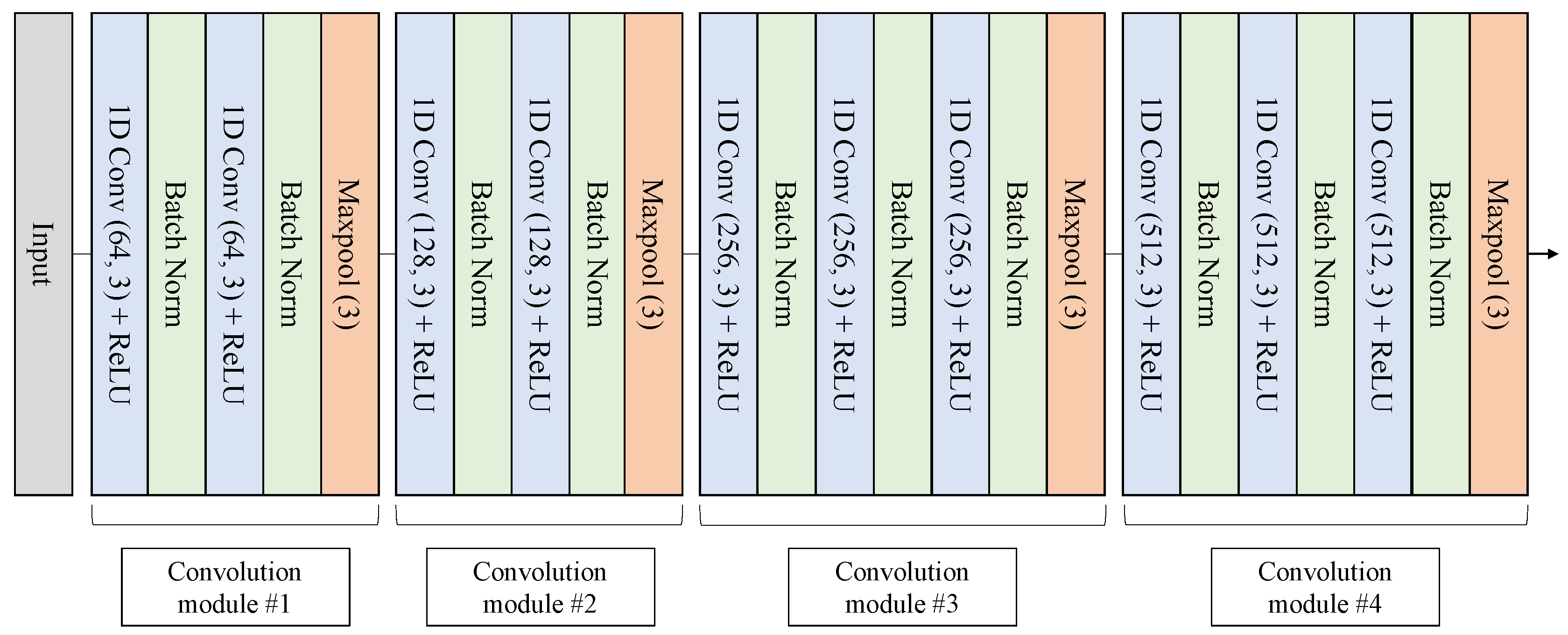
2.3.1. Convolutional Neural Network
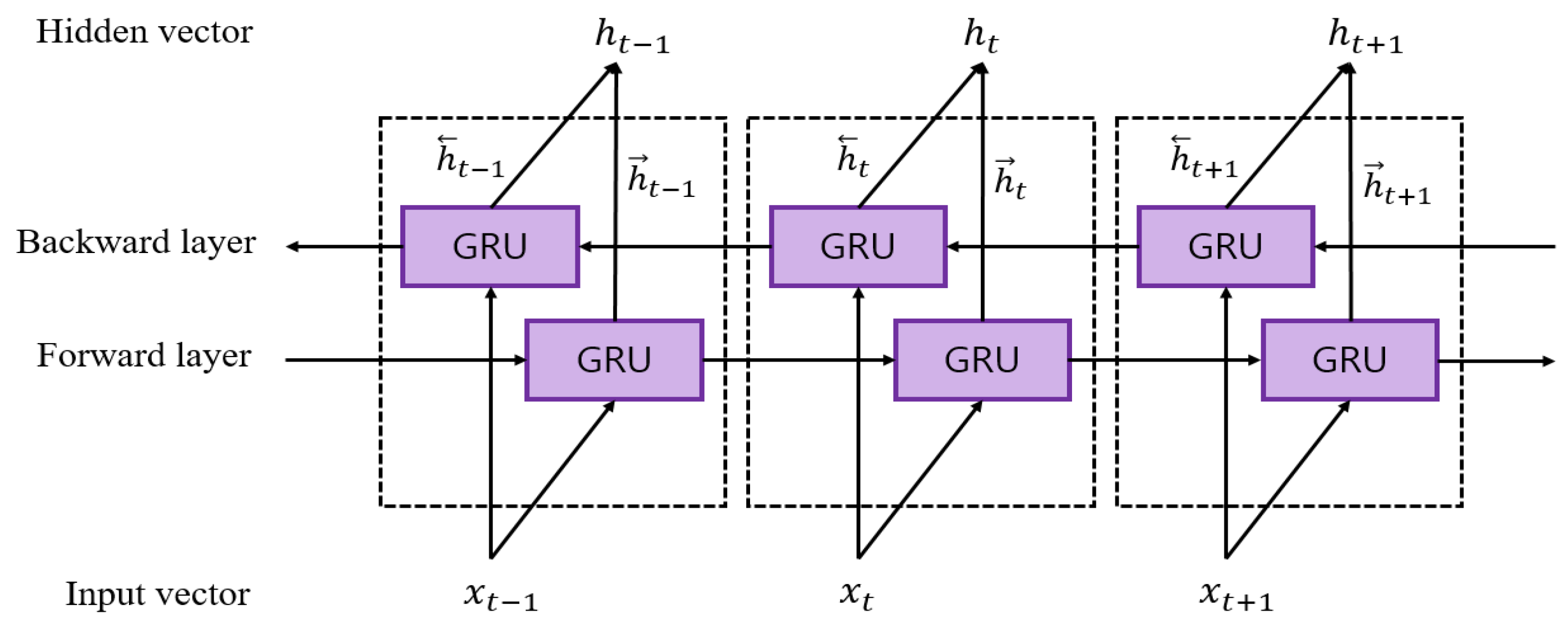
2.3.2. Bidirectional Gated Recurrent Unit
2.3.3. Attention Mechanism
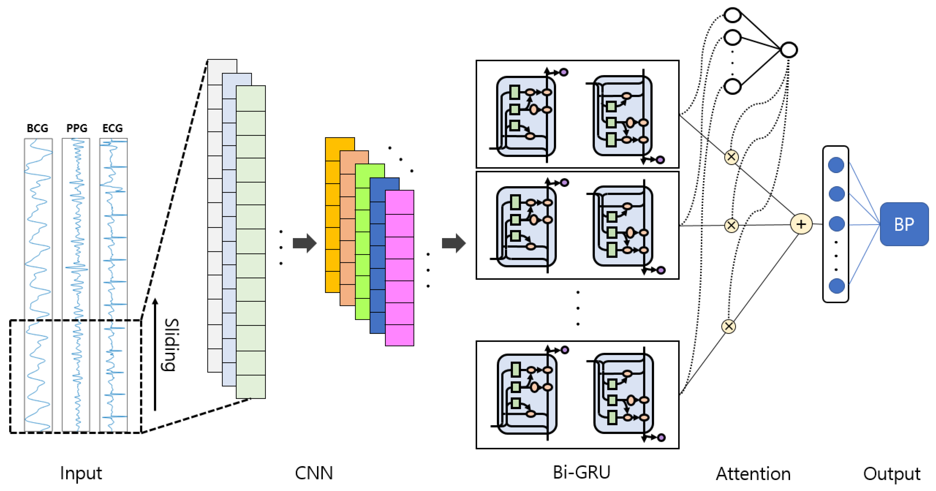
2.4. Proposed Model
2.4.1. Model Architecture
2.4.2. Training Setting
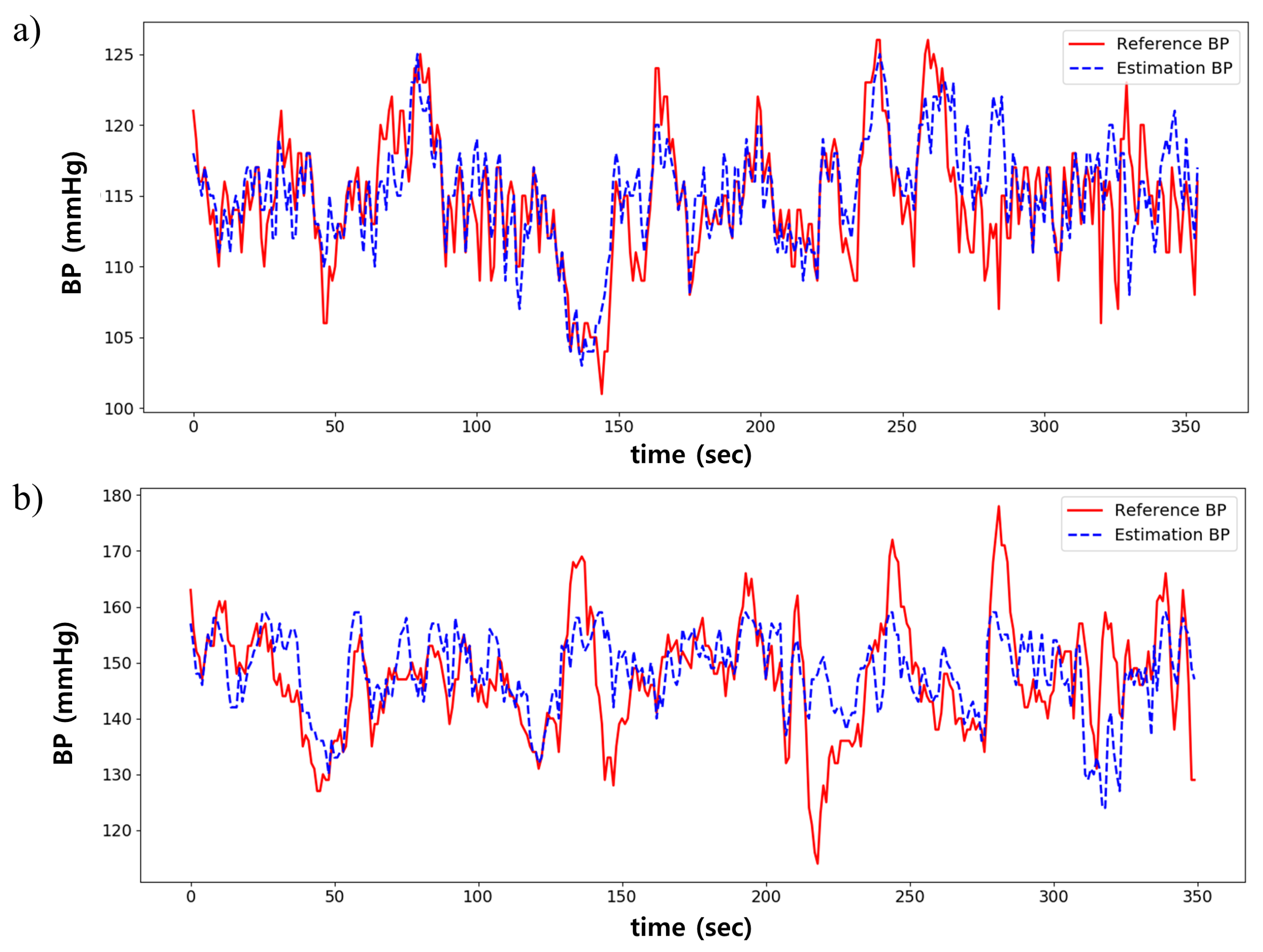
3. Results
3.1. Performance Comparison by Signal Combination
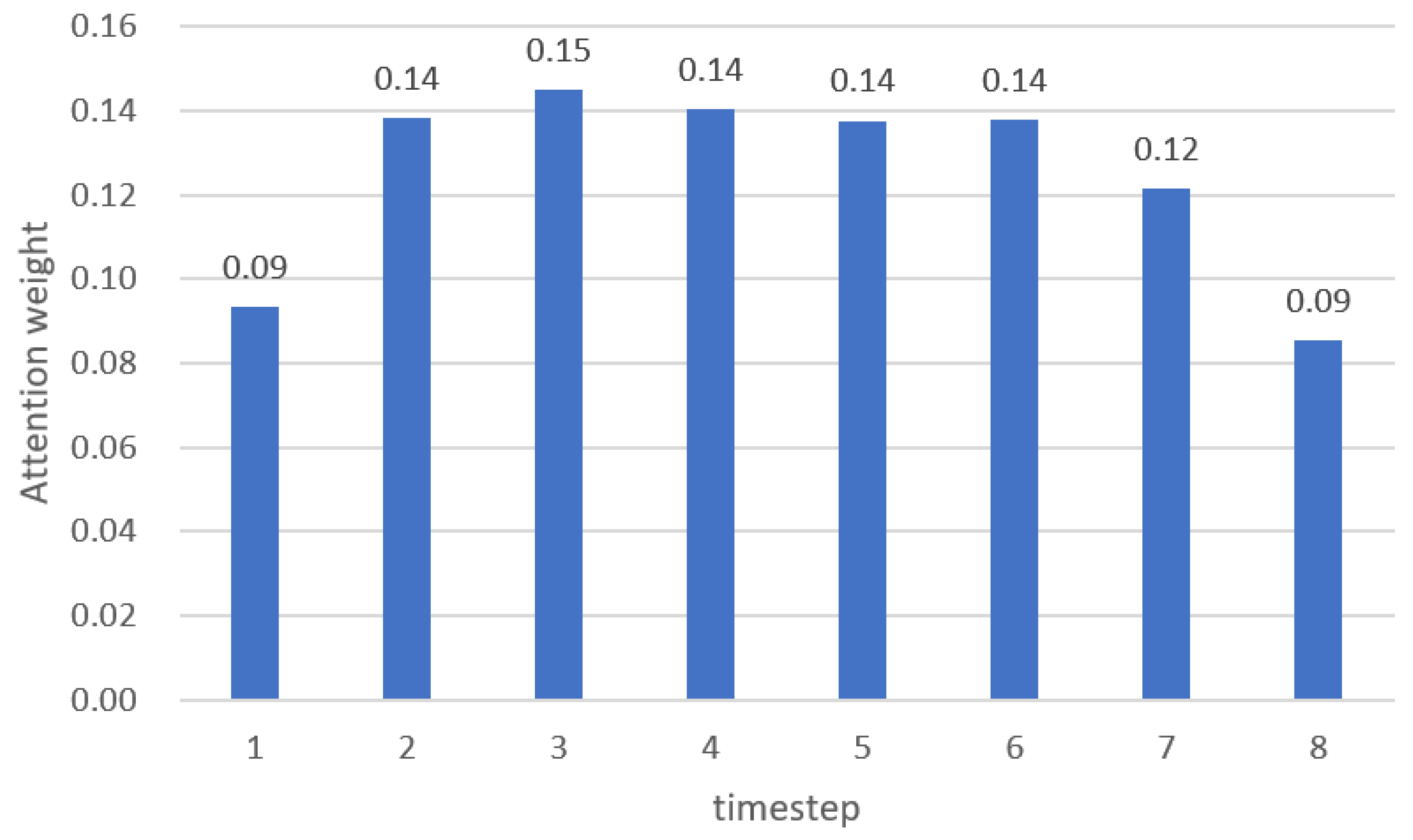
3.2. Attention Mechanism Performance
3.3. Comparison to the Multiple Linear Regression Model
4. Discussion
4.1. Main Contributions
4.2. Result Interpretation from Global Standard Perspective of BP Monitoring
4.3. Comparison Result With Related Works
4.4. Limitations of the Study
5. Conclusions and Future Work
Author Contributions
Funding
Conflicts of Interest
Abbreviations
| BP | Blood pressure |
| SBP | Systolic blood pressure |
| DBP | Diastolic blood pressure |
| ABP | Arterial blood pressure |
| ICU | Intensive care unit |
| PWV | Pulse wave velocity |
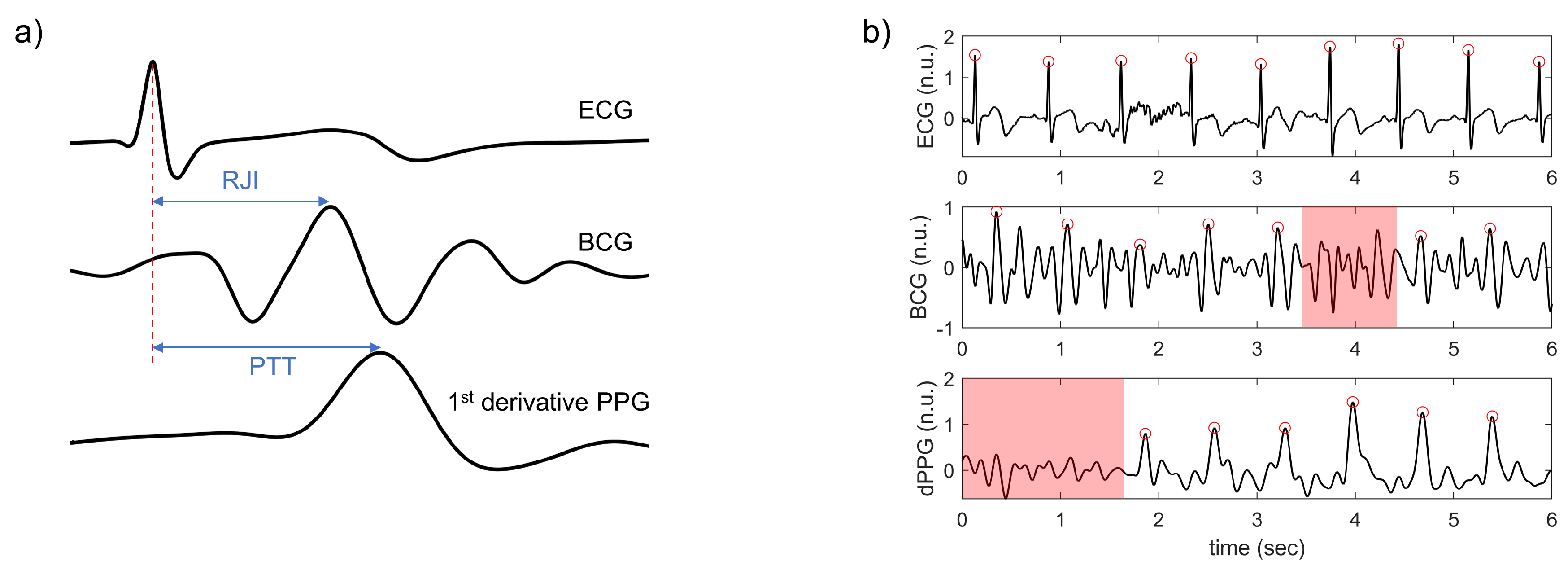
| PTT | Pulse transit time |
| ECG | Electrocardiogram |
| PPG | Photoplethysmogram |
| BCG | Ballistocardiogram |
| PVDF | Polyvinylidene fluoride |
| RJI | R-J interval |
| ANN | Artificial neural network |
| MLR | Multiple linear regression |
| RRI | R-R interval |
| CNN | Convolutional neural network |
| Bi-GRU | Bidirectional gated unit |
| ReLU | Rectified linear unit |
| RNN | Recurrent neural network |
| LSTM | Long short term memory |
| MLP | Multilayer perceptron |
| MSE | Mean squared error |
| MIMIC | Medical Information Mart for Intensive Care |
| RMSE | Root mean square error |
| MAE | Mean absolute error |
| SD | Standard deviation |
| ANOVA | Analysis of variance |
| LOA | Limits of agreement |
| AAMI | US Association for the Advancement of Medical Instrumentation |
| BHS | British Hypertension Society |
| LOSO | Leave-one-subject-out |
References
- World Health Organization (WHO), Hypertension. Available online: https://www.who.int/news-room/fact-sheets/detail/hypertension (accessed on 18 April 2020).
- Ogedegbe, G.; Pickering, T. Principles and techniques of blood pressure measurement. Cardiol. Clin. 2010, 28, 571–586. [Google Scholar] [CrossRef] [PubMed]
- Yoo, S.; Baek, H.; Doh, K.; Jeong, J.; Ahn, S.; Oh, I.Y.; Kim, K. Validation of the mobile wireless digital automatic blood pressure monitor using the cuff pressure oscillometric method, for clinical use and self-management, according to international protocols. Open Biomed. Eng. Lett. 2018, 8, 399–404. [Google Scholar] [CrossRef] [PubMed]
- Wu, D.; Xu, L.; Abbott, D.; Hau, W.K.; Ren, L.; Zhang, H.; Wong, K.K. Analysis of beat-to-beat blood pressure variability response to the cold pressor test in the offspring of hypertensive and normotensive parents. Hypertens. Res. 2017, 40, 581–589. [Google Scholar] [CrossRef] [PubMed]
- Ding, X.; Zhang, Y.T. Pulse transit time technique for cuffless unobtrusive blood pressure measurement: From theory to algorithm. Biomed. Eng. Lett. 2019, 9, 37–52. [Google Scholar] [CrossRef] [PubMed]
- Wong, M.Y.M.; Poon, C.C.Y.; Zhang, Y.T. An evaluation of the cuffless blood pressure estimation based on pulse transit time technique: A half year study on normotensive subjects. Cardiovasc. Eng. 2009, 9, 32–38. [Google Scholar] [CrossRef]
- Chen, W.; Kobayashi, T.; Ichikawa, S.; Takeuchi, Y.; Togawa, T. Continuous estimation of systolic blood pressure using the pulse arrival time and intermittent calibration. Med. Biol. Eng. Comput. 2000, 38, 569–574. [Google Scholar] [CrossRef]
- Poon, C.; Zhang, Y. Cuff-less and noninvasive measurements of arterial blood pressure by pulse transit time. In Proceedings of the 2005 IEEE Engineering in Medicine and Biology 27th Annual Conference, Shanghai, China, 17–18 January 2006; pp. 5877–5880. [Google Scholar]
- Baek, H.J.; Chung, G.S.; Kim, K.K.; Park, K.S. A smart health monitoring chair for nonintrusive measurement of biological signals. IEEE Trans. Inf. Technol. Biomed. 2011, 16, 150–158. [Google Scholar] [CrossRef]
- Ding, X.R.; Zhang, Y.T.; Liu, J.; Dai, W.X.; Tsang, H.K. Continuous cuffless blood pressure estimation using pulse transit time and photoplethysmogram intensity ratio. IEEE Trans. Biomed. Eng. 2016, 63, 964–972. [Google Scholar] [CrossRef]
- Kim, C.S.; Carek, A.M.; Mukkamala, R.; Inan, O.T.; Hahn, J.O. Ballistocardiogram as proximal timing reference for pulse transit time measurement: Potential for cuffless blood pressure monitoring. IEEE Trans. Biomed. Eng. 2015, 62, 2657–2664. [Google Scholar] [CrossRef]
- Shin, J.H.; Lee, K.M.; Park, K.S. Non-constrained monitoring of systolic blood pressure on a weighing scale. Physiol. Meas. 2009, 30, 679. [Google Scholar] [CrossRef]
- Lee, K.J.; Roh, J.; Cho, D.; Hyeong, J.; Kim, S. A Chair-Based Unconstrained/Nonintrusive Cuffless Blood Pressure Monitoring System Using a Two-Channel Ballistocardiogram. Sensors 2019, 19, 595. [Google Scholar] [CrossRef]
- Chan, K.; Hung, K.; Zhang, Y. Noninvasive and cuffless measurements of blood pressure for telemedicine. In Proceedings of the 23rd Annual International Conference of the IEEE Engineering in Medicine and Biology Society, Istanbul, Turkey, 25–28 October 2001; pp. 3592–3593. [Google Scholar]
- Kachuee, M.; Kiani, M.M.; Mohammadzade, H.; Shabany, M. Cuffless blood pressure estimation algorithms for continuous health-care monitoring. IEEE Trans. Biomed. Eng. 2016, 64, 859–869. [Google Scholar] [CrossRef] [PubMed]
- Su, P.; Ding, X.R.; Zhang, Y.T.; Liu, J.; Miao, F.; Zhao, N. Long-term blood pressure prediction with deep recurrent neural networks. In Proceedings of the 2018 IEEE EMBS International Conference on Biomedical & Health Informatics (BHI), Las Vegas, NV, USA, 4–7 March 2018; pp. 323–328. [Google Scholar]
- Kurylyak, Y.; Lamonaca, F.; Grimaldi, D. A Neural Network-based method for continuous blood pressure estimation from a PPG signal. In Proceedings of the 2013 IEEE International Instrumentation and Measurement Technology Conference (I2MTC), Minneapolis, MN, USA, 6–9 May 2013; pp. 280–283. [Google Scholar]
- Wang, L.; Zhou, W.; Xing, Y.; Zhou, X. A novel neural network model for blood pressure estimation using photoplethesmography without electrocardiogram. J. Healthcare Eng. 2018, 2018. [Google Scholar] [CrossRef] [PubMed]
- Slapničar, G.; Mlakar, N.; Luštrek, M. Blood Pressure Estimation from Photoplethysmogram Using a Spectro-Temporal Deep Neural Network. Sensors 2019, 19, 3420. [Google Scholar] [CrossRef]
- Tanveer, M.S.; Hasan, M.K. Cuffless blood pressure estimation from electrocardiogram and photoplethysmogram using waveform based ANN-LSTM network. Biomed. Signal Process. Control 2019, 51, 382–392. [Google Scholar] [CrossRef]
- Physiolab, Busan, Korea. Available online: http://www.physiolab.co.kr (accessed on 18 April 2020).
- Goldberger, A.L.; Amaral, L.A.; Glass, L.; Hausdorff, J.M.; Ivanov, P.C.; Mark, R.G.; Mietus, J.E.; Moody, G.B.; Peng, C.K.; Stanley, H.E.; et al. PhysioBank, PhysioToolkit, and PhysioNet: Components of a new research resource for complex physiologic signals. Circulation 2000, 101, e215–e220. [Google Scholar] [CrossRef]
- Wen, X.; Huang, Y.; Wu, X.M.; Zhang, B. A Feasible Feature Extraction Method for Atrial Fibrillation Detection from BCG. IEEE J. Biomed. Health Inf. 2019, 24, 1093–1103. [Google Scholar] [CrossRef]
- Rundo, F.; Conoci, S.; Ortis, A.; Battiato, S. An advanced bio-inspired photoplethysmography (PPG) and ECG pattern recognition system for medical assessment. Sensors 2018, 18, 405. [Google Scholar] [CrossRef]
- Yıldırım, Ö.; Pławiak, P.; Tan, R.S.; Acharya, U.R. Arrhythmia detection using deep convolutional neural network with long duration ECG signals. Comput. Biol. Med. 2018, 102, 411–420. [Google Scholar] [CrossRef]
- Ullah, I.; Hussain, M.; Aboalsamh, H. An automated system for epilepsy detection using EEG brain signals based on deep learning approach. Expert Syst. Appl. 2018, 107, 61–71. [Google Scholar] [CrossRef]
- Dey, D.; Chaudhuri, S.; Munshi, S. Obstructive sleep apnoea detection using convolutional neural network based deep learning framework. Biomed. Eng. Lett. 2018, 8, 95–100. [Google Scholar] [CrossRef] [PubMed]
- Khagi, B.; Lee, B.; Pyun, J.Y.; Kwon, G.R. CNN Models Performance Analysis on MRI images of OASIS dataset for distinction between Healthy and Alzheimer’s patient. In Proceedings of the 2019 International Conference on Electronics, Information, and Communication (ICEIC), Auckland, New Zealand, 22–25 January 2019; pp. 1–4. [Google Scholar]
- Bengio, Y.; Simard, P.; Frasconi, P. Learning long-term dependencies with gradient descent is difficult. IEEE Trans. Neural Networks 1994, 5, 157–166. [Google Scholar] [CrossRef] [PubMed]
- Hochreiter, S.; Schmidhuber, J. Long short-term memory. Neural Comput. 1997, 9, 1735–1780. [Google Scholar] [CrossRef] [PubMed]
- Cho, K.; Van Merriënboer, B.; Gulcehre, C.; Bahdanau, D.; Bougares, F.; Schwenk, H.; Bengio, Y. Learning phrase representations using RNN encoder-decoder for statistical machine translation. arXiv 2014, arXiv:1406.1078. [Google Scholar]
- Chung, J.; Gulcehre, C.; Cho, K.; Bengio, Y. Empirical evaluation of gated recurrent neural networks on sequence modeling. arXiv 2014, arXiv:1412.3555. [Google Scholar]
- Xu, K.; Ba, J.; Kiros, R.; Cho, K.; Courville, A.; Salakhudinov, R.; Zemel, R.; Bengio, Y. Show, attend and tell: Neural image caption generation with visual attention. In Proceedings of the International Conference on Machine Learning, Lille, France, 6–11 July 2015; pp. 2048–2057. [Google Scholar]
- Luong, M.T.; Pham, H.; Manning, C.D. Effective approaches to attention-based neural machine translation. arXiv 2015, arXiv:1508.04025. [Google Scholar]
- Bahdanau, D.; Cho, K.; Bengio, Y. Neural machine translation by jointly learning to align and translate. arXiv 2014, arXiv:1409.0473. [Google Scholar]
- Song, H.; Rajan, D.; Thiagarajan, J.J.; Spanias, A. Attend and Diagnose: Clinical Time Series Analysis Using Attention Models. In Proceedings of the Thirty-second AAAI conference on artificial intelligence, New Orleans, LA, USA, 2–7 February 2018. [Google Scholar]
- Chaudhari, S.; Polatkan, G.; Ramanath, R.; Mithal, V. An attentive survey of attention models. arXiv 2019, arXiv:1904.02874. [Google Scholar]
- Raffel, C.; Ellis, D.P. Feed-forward networks with attention can solve some long-term memory problems. arXiv 2015, arXiv:1512.08756. [Google Scholar]
- Shi, B.; Bai, X.; Yao, C. An end-to-end trainable neural network for image-based sequence recognition and its application to scene text recognition. IEEE Trans. Pattern Anal. Mach. Intell. 2016, 39, 2298–2304. [Google Scholar] [CrossRef]
- Oh, S.L.; Ng, E.Y.; San Tan, R.; Acharya, U.R. Automated diagnosis of arrhythmia using combination of CNN and LSTM techniques with variable length heart beats. Comput. Biol. Med. 2018, 102, 278–287. [Google Scholar] [CrossRef] [PubMed]
- Kim, Y.; Yeo, M.; Sohn, I.; Park, C. Multimodal drowsiness detection methods using machine learning algorithms. IEIE Trans. Smart Process. Comput. 2018, 7, 361–365. [Google Scholar] [CrossRef]
- Seok, W.; Park, C. Recognition of Human Motion with Deep Reinforcement Learning. IEIE Trans. Smart Process. Comput. 2018, 7, 245–250. [Google Scholar] [CrossRef]
- Vaswani, A.; Shazeer, N.; Parmar, N.; Uszkoreit, J.; Jones, L.; Gomez, A.N.; Kaiser, Ł.; Polosukhin, I. Attention Is All You Need. In Proceedings of the Advances in Neural Information Processing Systems, Long Beach, CA, USA, 4–9 December 2017; pp. 5998–6008. [Google Scholar]
- Simonyan, K.; Zisserman, A. Very deep convolutional networks for large-scale image recognition. arXiv 2014, arXiv:1409.1556. [Google Scholar]
- Ioffe, S.; Szegedy, C. Batch normalization: Accelerating deep network training by reducing internal covariate shift. arXiv 2015, arXiv:1502.03167. [Google Scholar]
- Kingma, D.P.; Ba, J. Adam: A method for stochastic optimization. arXiv 2014, arXiv:1412.6980. [Google Scholar]
- Altman, D.G.; Bland, J.M. Measurement in medicine: The analysis of method comparison studies. J. R. Stat. Soc. Ser. D 1983, 32, 307–317. [Google Scholar] [CrossRef]
- Pan, J.; Tompkins, W.J. A real-time QRS detection algorithm. IEEE Trans. Biomed. Eng. 1985, 230–236. [Google Scholar] [CrossRef]
- Association for the Advancement of Medical Instrumentation. American National Standards for Electronic or automated sphygmomanometers. ANSI AAMI 1992, 1–40. [Google Scholar]
- O’Brien, E.; Petrie, J.; Littler, W.; de Swiet, M.; Padfield, P.L.; Altman, D.; Bland, M.; Coats, A.; Atkins, N. The British Hypertension Society protocol for the evaluation of blood pressure measuring devices. J. Hypertens. 1993, 11, S43–S62. [Google Scholar]
- Whelton, P.K.; Carey, R.M. The 2017 American College of Cardiology/American Heart Association clinical practice guideline for high blood pressure in adults. JAMA Cardiol. 2018, 3, 352–353. [Google Scholar] [CrossRef] [PubMed]


| Signal | HPF (Hz) | LPF (Hz) |
|---|---|---|
| ECG | 0.5 | 35 |
| BCG | 4 | 15 |
| PPG | 0.5 | 15 |
| Network | Layer | Shape | Out | Padding | Stride | Kernel |
|---|---|---|---|---|---|---|
| CNN | Conv | 64 | Same | 1 | 3 | |
| BN + ReLU | ||||||
| Conv | 64 | Same | 1 | 3 | ||
| BN + ReLU | ||||||
| Maxpool (size = 3) | - | Same | 3 | - | ||
| Conv | 128 | Same | 1 | 3 | ||
| BN + ReLU | ||||||
| Conv | 128 | Same | 1 | 3 | ||
| BN + ReLU | ||||||
| Maxpool (size = 3) | - | Same | 3 | - | ||
| Conv | 256 | Same | 1 | 3 | ||
| BN + ReLU | ||||||
| Conv | 256 | Same | 1 | 3 | ||
| BN + ReLU | ||||||
| Conv | 256 | Same | 1 | 3 | ||
| BN + ReLU | ||||||
| Maxpool (size = 3) | - | Same | 3 | - | ||
| Conv | 512 | Same | 1 | 3 | ||
| BN + ReLU | ||||||
| Conv | 512 | Same | 1 | 3 | ||
| BN + ReLU | ||||||
| Conv | 512 | Same | 1 | 3 | ||
| BN + ReLU | ||||||
| Maxpool (size = 3) | - | Same | 3 | - | ||
| Bi-GRU | Forward | 64 | - | |||
| Backward | 64 | - | ||||
| Concatenation | ||||||
| Attention | 1-layer perceptron | 1 | - | |||
| Activation tanh | ||||||
| Softmax | ||||||
| Weighted sum | ||||||
| 1-layer perceptron | 128 | 2 | - | |||
| Model | Input | SBP (mmHg) | DBP (mmHg) | ||||||
|---|---|---|---|---|---|---|---|---|---|
| RMSE | MAE | SD | RMSE | MAE | SD | ||||
| CNN+Bi-GRU | ECG | 7.02 | 5.51 | 4.66 | 0.24 | 5.16 | 4.06 | 3.45 | 0.27 |
| PPG | 6.88 | 5.34 | 4.60 | 0.28 | 5.73 | 4.45 | 4.09 | 0.14 | |
| BCG | 7.24 | 5.59 | 5.03 | 0.20 | 5.29 | 4.06 | 3.71 | 0.22 | |
| ECG, PPG | 5.83 | 4.46 | 4.06 | 0.46 | 4.74 | 3.70 | 3.37 | 0.38 | |
| ECG, BCG | 6.74 | 5.30 | 4.60 | 0.31 | 4.82 | 3.74 | 3.27 | 0.34 | |
| PPG, BCG | 6.44 | 4.86 | 4.50 | 0.36 | 5.04 | 3.88 | 3.62 | 0.27 | |
| ECG, PPG, BCG | 5.87 | 4.51 | 4.14 | 0.48 | 4.73 | 3.71 | 3.39 | 0.40 | |
| CNN+Bi-GRU +Attention (proposed model) | ECG, PPG, BCG | 5.42 [1.97, 8.87] | 4.06 [1.53, 6.59] | 4.04 | 0.52 | 4.30 [0.94, 7.72] | 3.33 [0.61, 6.05] | 3.42 | 0.49 |
| Input | SBP (mmHg) | DBP (mmHg) | ||||
|---|---|---|---|---|---|---|
| RMSE | MAE | mean | RMSE | MAE | mean | |
| Single signal | 7.04 | 5.47 | 0.24 | 5.39 | 4.19 | 0.21 |
| Multiple signals | 6.21 | 4.78 | 0.40 | 4.83 | 3.76 | 0.35 |
| Inputs | ECG | PPG | BCG | ECG, PPG | ECG, BCG | BCG, PPG | ECG, BCG, PPG | Proposed Model |
|---|---|---|---|---|---|---|---|---|
| ECG | - | - | p < 0.05 | - | - | p < 0.05 | p < 0.05 | |
| PPG | - | p < 0.05 | - | p < 0.05 | p < 0.05 | p < 0.05 | ||
| BCG | p < 0.05 | - | p < 0.05 | p < 0.05 | p < 0.05 | |||
| ECG, PPG | p < 0.05 | - | - | p < 0.05 | ||||
| ECG, BCG | - | p < 0.05 | p < 0.05 | |||||
| BCG, PPG | - | p < 0.05 | ||||||
| ECG, BCG, PPG | p < 0.05 |
| Inputs | ECG | PPG | BCG | ECG, PPG | ECG, BCG | BCG, PPG | ECG, BCG, PPG | Proposed Model |
|---|---|---|---|---|---|---|---|---|
| ECG | - | - | - | p < 0.05 | - | - | p < 0.05 | |
| PPG | - | p < 0.05 | p < 0.05 | p < 0.05 | p < 0.05 | p < 0.05 | ||
| BCG | - | - | - | - | p < 0.05 | |||
| ECG, PPG | - | - | - | p < 0.05 | ||||
| ECG, BCG | - | - | p < 0.05 | |||||
| BCG, PPG | - | p < 0.05 | ||||||
| ECG, BCG, PPG | p < 0.05 |
| Model | SBP (mmHg) | DBP (mmHg) | ||||||
|---|---|---|---|---|---|---|---|---|
| RMSE | MAE | SD | RMSE | MAE | SD | |||
| Proposed model | 5.42 | 4.06 | 4.04 | 0.52 | 4.30 | 3.33 | 3.42 | 0.49 |
| MLR | 6.40 | 5.19 | 3.45 | 0.26 | 4.75 | 3.85 | 2.69 | 0.22 |
| Mean Error | Standard Deviation | ||
|---|---|---|---|
| AAMI standard | SBP, DBP | ≤ 5 (mmHg) | ≤ 8 (mmHg) |
| Proposed model | SBP | −0.20 | 5.83 |
| DBP | −0.02 | 4.91 |
| Absolute Difference | Grade | ||||
|---|---|---|---|---|---|
| ≤ 5 (mmHg) | ≤ 10 (mmHg) | ≤ 15 (mmHg) | |||
| BHS standard | SBP, DBP | 60% | 85% | 95% | A |
| 50% | 75% | 90% | B | ||
| 40% | 65% | 80% | C | ||
| Worse than C | D | ||||
| Proposed model | SBP | 73% | 93% | 98% | A |
| DBP | 80% | 96% | 99% | A | |
| Author | Data Size | Calibration | Model | Input | SBP (mmHg) | DBP (mmHg) | |
|---|---|---|---|---|---|---|---|
| Inputs | Signal | Error | Error | ||||
| Chan et al. [14] | Unspecified | Cal-based | Linear regression | Feature (PTT) | ECG PPG | ME: 7.49 STD: 8.82 | ME: 4.08 STD: 5.62 |
| Kachuee et al. [15] | 1000 subjects 10 min (MIMIC 3) | Cal-based | AdaBoost | Features | ECG PPG | MAE: 8.21 STD: 5.45 | MAE: 4.31 STD: 3.52 |
| Cal-free | MAE: 11.17 STD: 10.09 | MAE: 5.35 STD: 6.14 | |||||
| Kurylyak et al. [17] | 15,000 heartbeats | Cal-based | Deep learning (ANN) | Features | PPG | ME: 3.80 STD: 3.46 | ME: 2.21 STD: 2.09 |
| Lee et al. [13] | 30 subjects | Cal-based | Deep learning (ANN) | Feature (IPD) | BCG | ME: 0.01 STD: 6.75 | ME: 0.05 STD: 5.83 |
| Slapnivcar et al. [19] | 510 subjects 700 h (MIMIC 3) | Cal-based | Deep learning (ResNet) | Raw | PPG | MAE: 9.43 | MAE: 6.88 |
| Cal-free | MAE: 15.41 | MAE: 12.38 | |||||
| Su et al. [16] | 84 subjects 10 min | Cal-based | Deep learning (RNN) | Features | ECG PPG | RMSE: 3.73 | RMSE: 2.43 |
| Tanveer et al. [20] | 39 subjects (MIMIC 1) | Cal-based | Deep learning (ANN+ LSTM) | Raw | ECG PPG | RMSE: 1.27 MAE: 0.93 | RMSE: 0.73 MAE: 0.52 |
| Wang et al. [18] | 58,795 intervals of PPG (MIMIC 1) | Cal-based | Deep learning (ANN) | Features | PPG | MAE: 4.02 STD: 2.79 | MAE: 2.27 STD: 1.82 |
| This study | 15 subjects 30 min | Cal-based | Deep learning (CNN+ Bi-GRU) | Raw | BCG | ME: −0.82 STD: 7.50 | ME: −0.97 STD: 5.36 |
| ECG PPG | MAE: 4.46 STD: 4.06 | MAE: 3.70 STD: 3.37 | |||||
| Deep learning (CNN+ Bi-GRU+ Attention) | ECG PPG BCG | MAE: 4.06 STD: 4.04 | MAE: 3.33 STD: 3.42 | ||||
| Input | Method | SBP (mmHg) | DBP (mmHg) | ||||||
|---|---|---|---|---|---|---|---|---|---|
| RMSE | MAE | SD | RMSE | MAE | SD | ||||
| ECG, PPG, BCG | Cal-based | 5.42 | 4.06 | 4.04 | 0.52 | 4.3 | 3.33 | 3.42 | 0.49 |
| Cal-free | 13.14 | 9.70 | 8.86 | 0.23 | 7.55 | 5.79 | 4.84 | 0.44 | |
© 2020 by the authors. Licensee MDPI, Basel, Switzerland. This article is an open access article distributed under the terms and conditions of the Creative Commons Attribution (CC BY) license (http://creativecommons.org/licenses/by/4.0/).
Share and Cite
Eom, H.; Lee, D.; Han, S.; Hariyani, Y.S.; Lim, Y.; Sohn, I.; Park, K.; Park, C. End-To-End Deep Learning Architecture for Continuous Blood Pressure Estimation Using Attention Mechanism. Sensors 2020, 20, 2338. https://doi.org/10.3390/s20082338
Eom H, Lee D, Han S, Hariyani YS, Lim Y, Sohn I, Park K, Park C. End-To-End Deep Learning Architecture for Continuous Blood Pressure Estimation Using Attention Mechanism. Sensors. 2020; 20(8):2338. https://doi.org/10.3390/s20082338
Chicago/Turabian StyleEom, Heesang, Dongseok Lee, Seungwoo Han, Yuli Sun Hariyani, Yonggyu Lim, Illsoo Sohn, Kwangsuk Park, and Cheolsoo Park. 2020. "End-To-End Deep Learning Architecture for Continuous Blood Pressure Estimation Using Attention Mechanism" Sensors 20, no. 8: 2338. https://doi.org/10.3390/s20082338
APA StyleEom, H., Lee, D., Han, S., Hariyani, Y. S., Lim, Y., Sohn, I., Park, K., & Park, C. (2020). End-To-End Deep Learning Architecture for Continuous Blood Pressure Estimation Using Attention Mechanism. Sensors, 20(8), 2338. https://doi.org/10.3390/s20082338