On the Identification of Elastic Moduli of In-Service Rail by Ultrasonic Guided Waves


Abstract
1. Introduction
2. Methodology for the Inversion Process
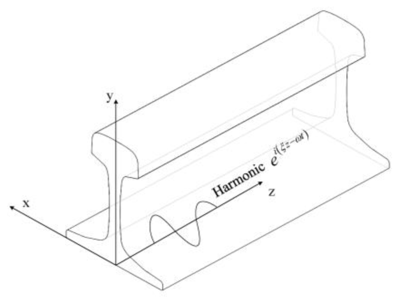
2.1. SAFE method for Estimating Guided Wave Propagation in Rail
2.2. Extraction Method of Phase Velocity
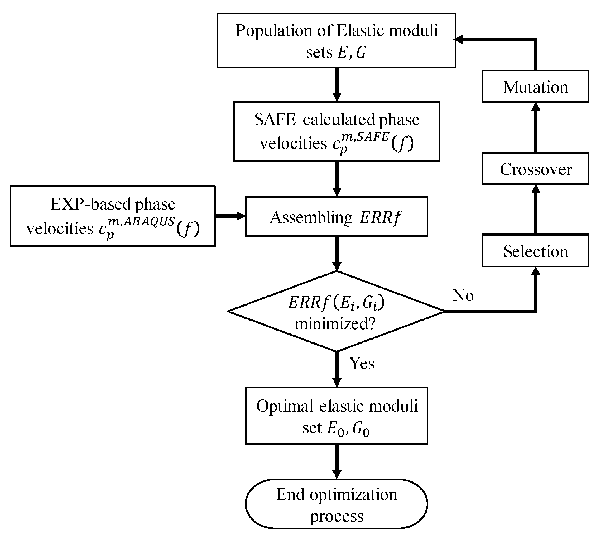
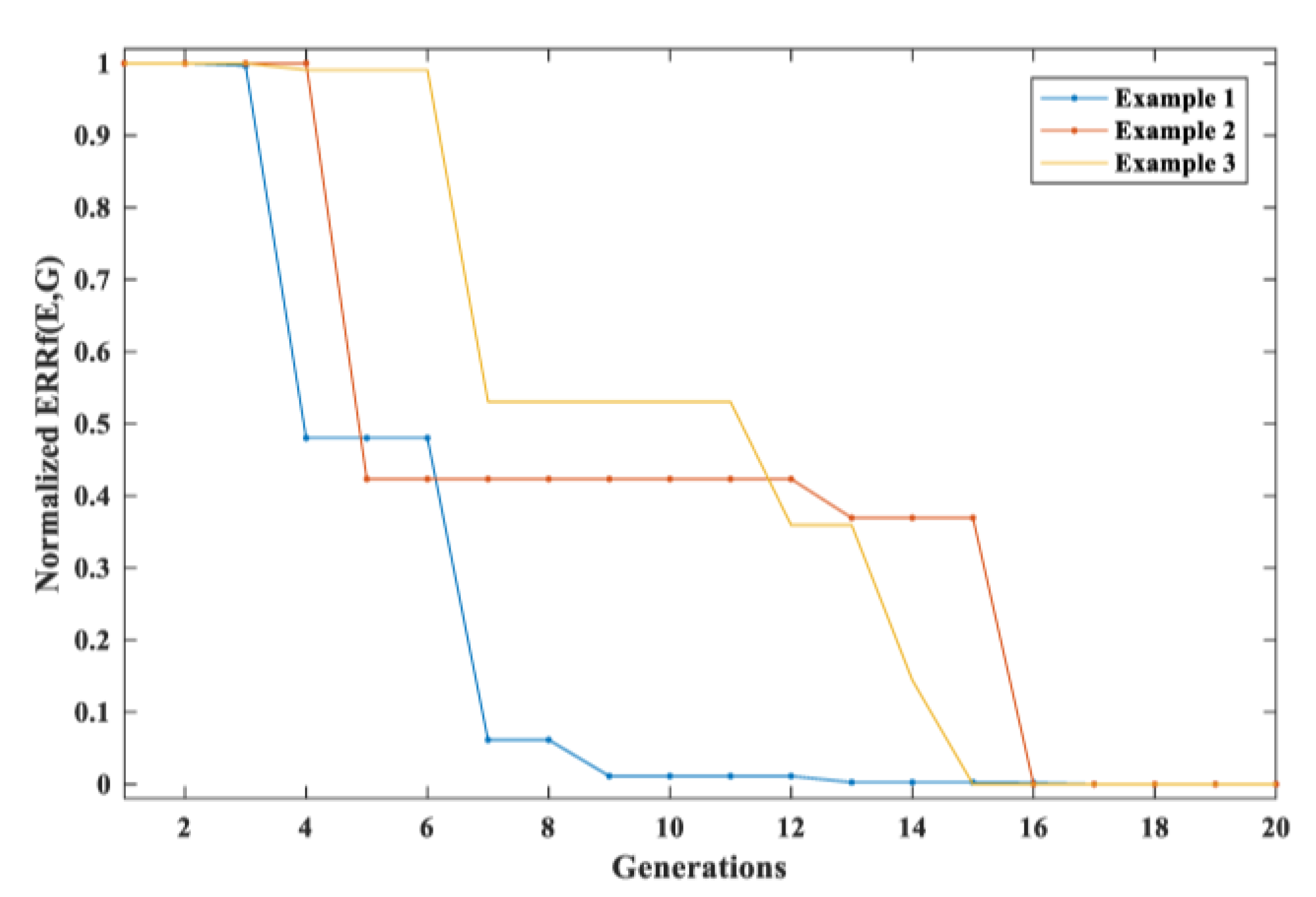
2.3. Optimization Approach for Identification of Elastic Constants
3. Mode Selection and Excitation Method
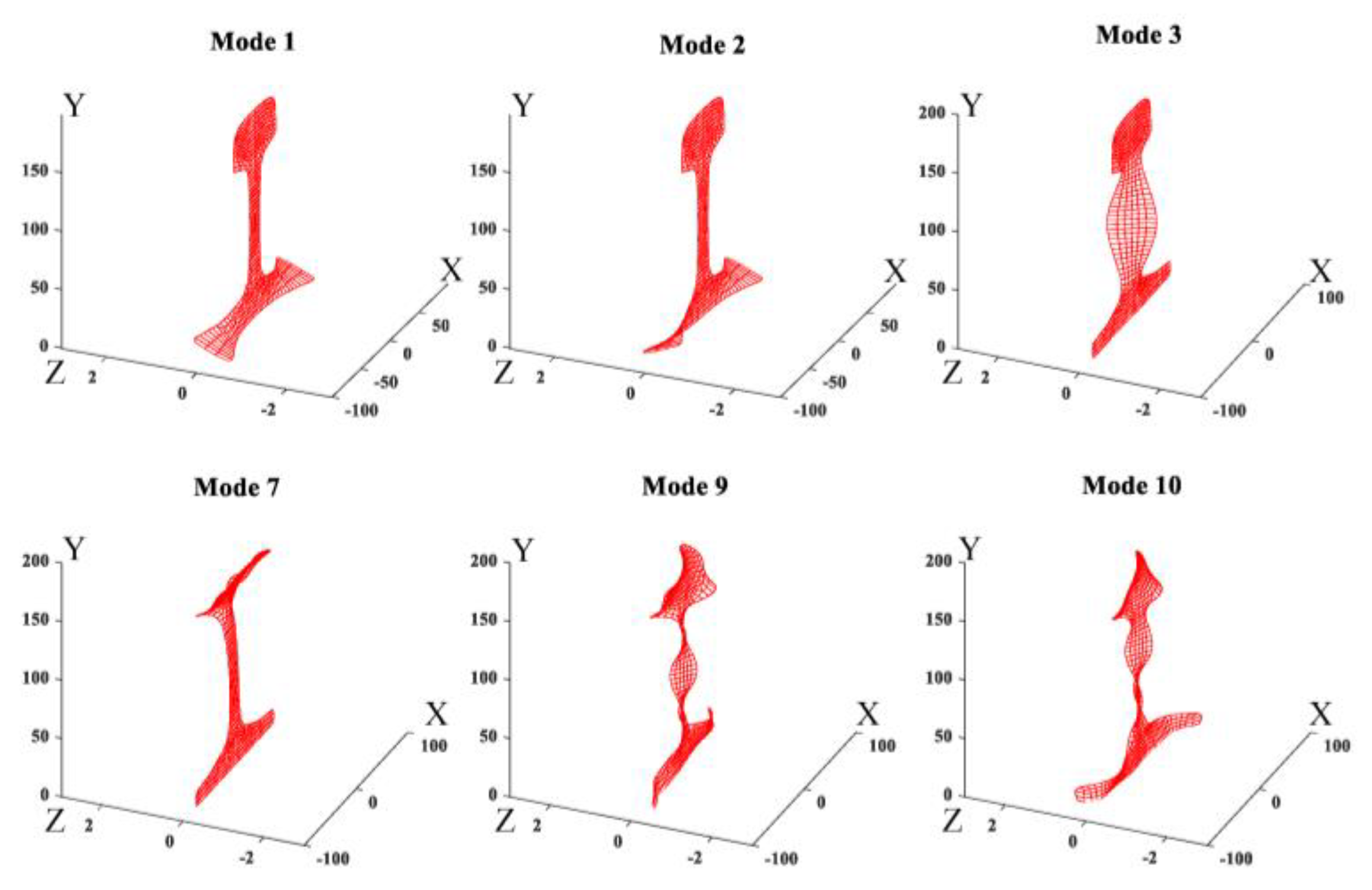
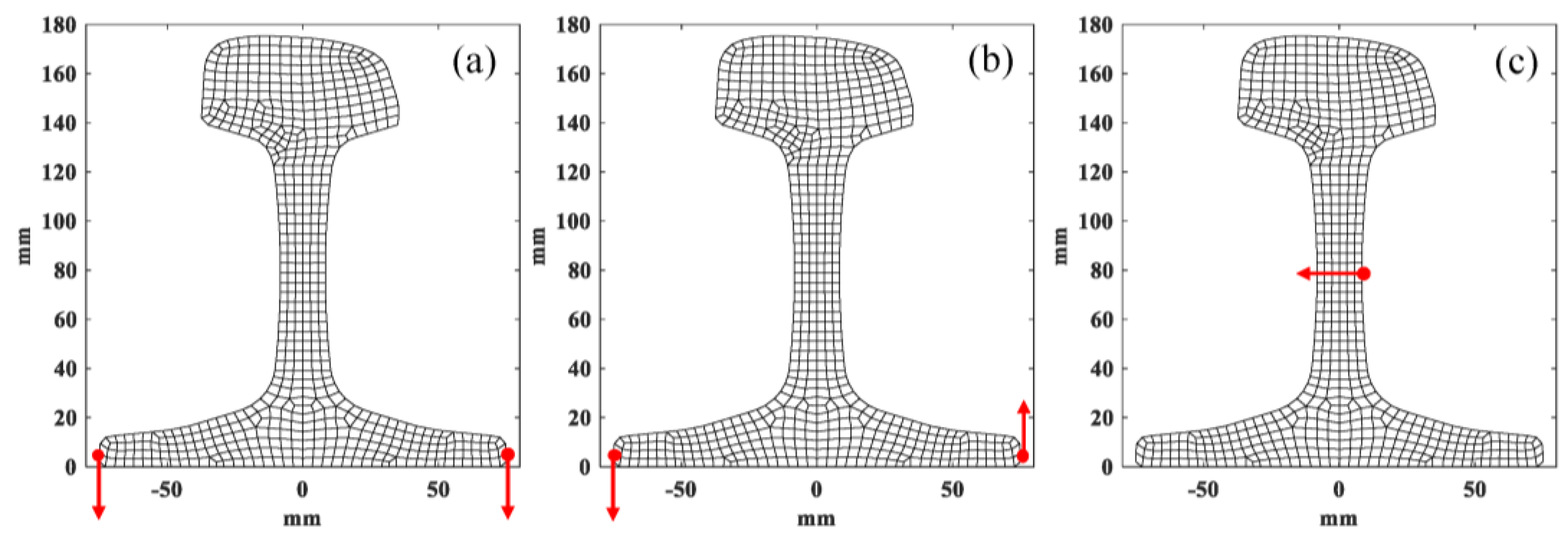
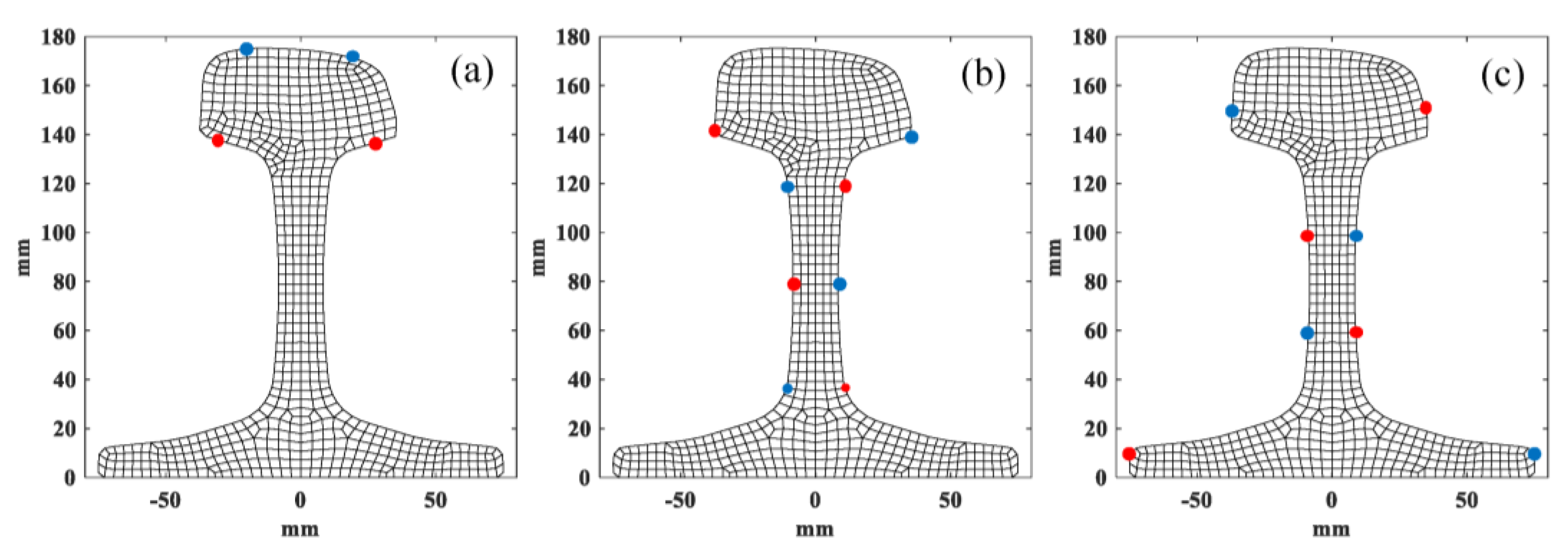
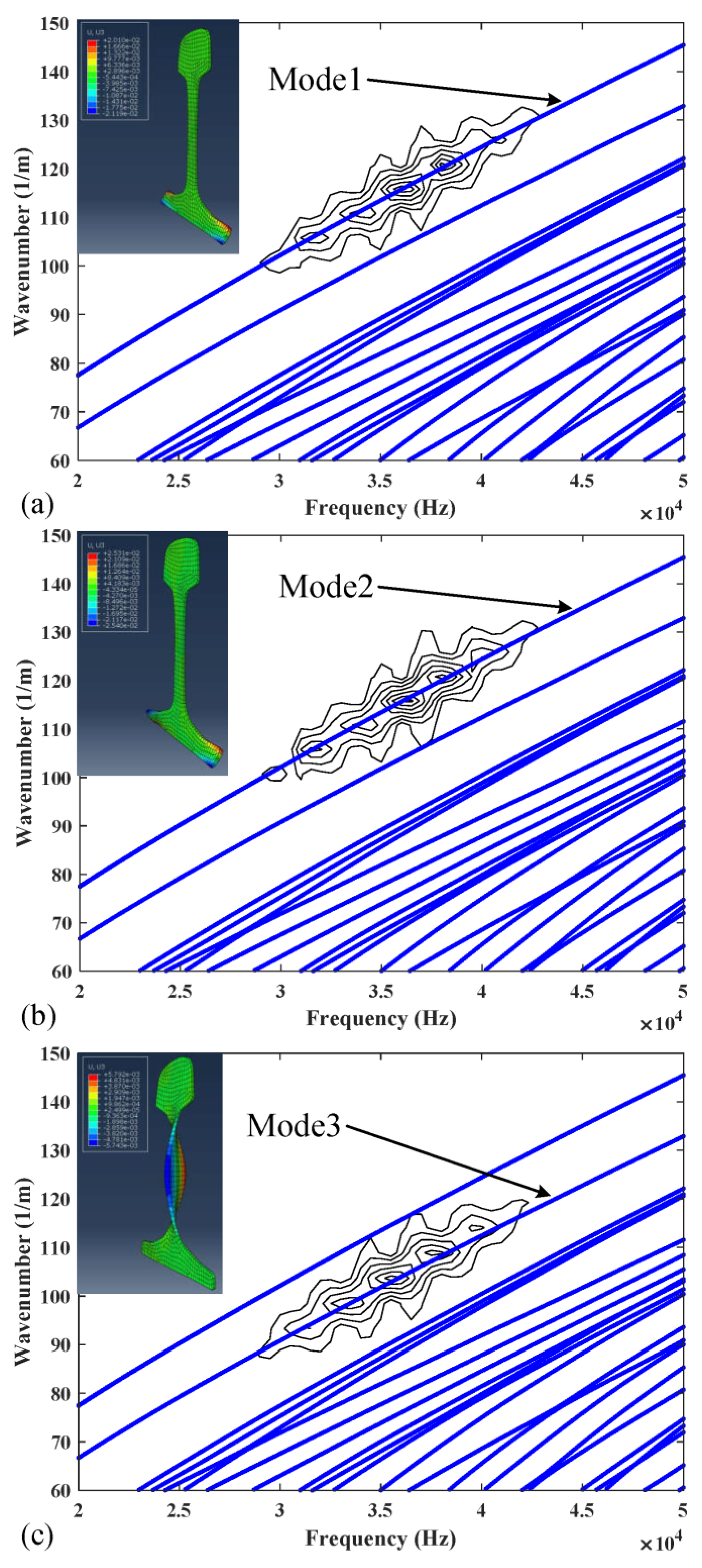
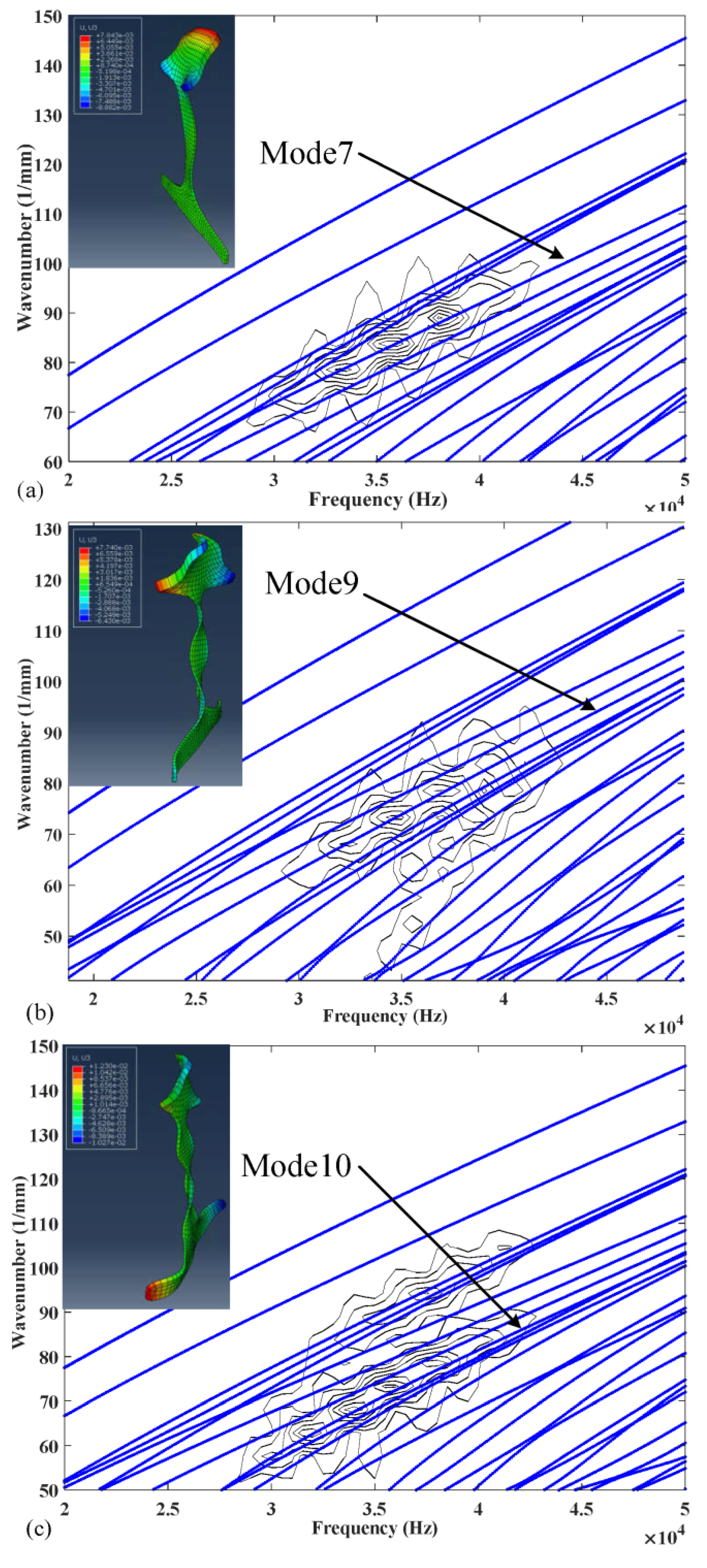
3.1. Mode Selection
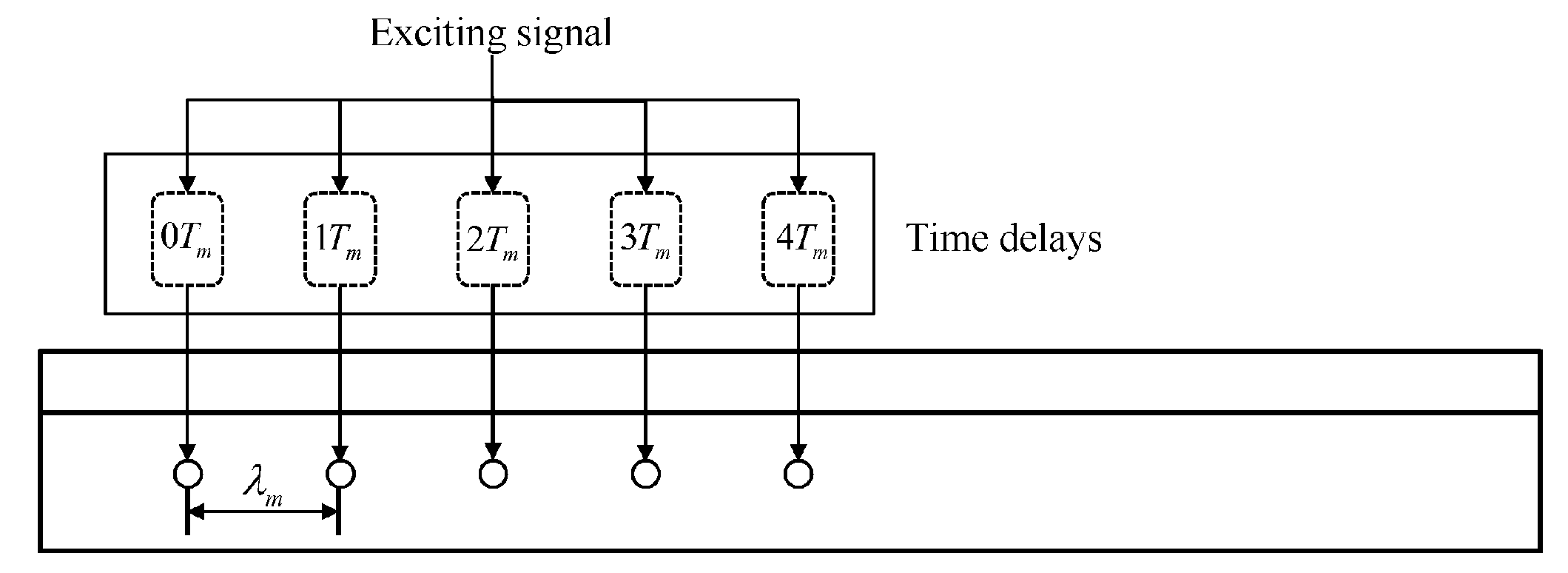
3.2. Excitation Method of Specific Mode
4. Numerical Validation: Finite Element Analysis
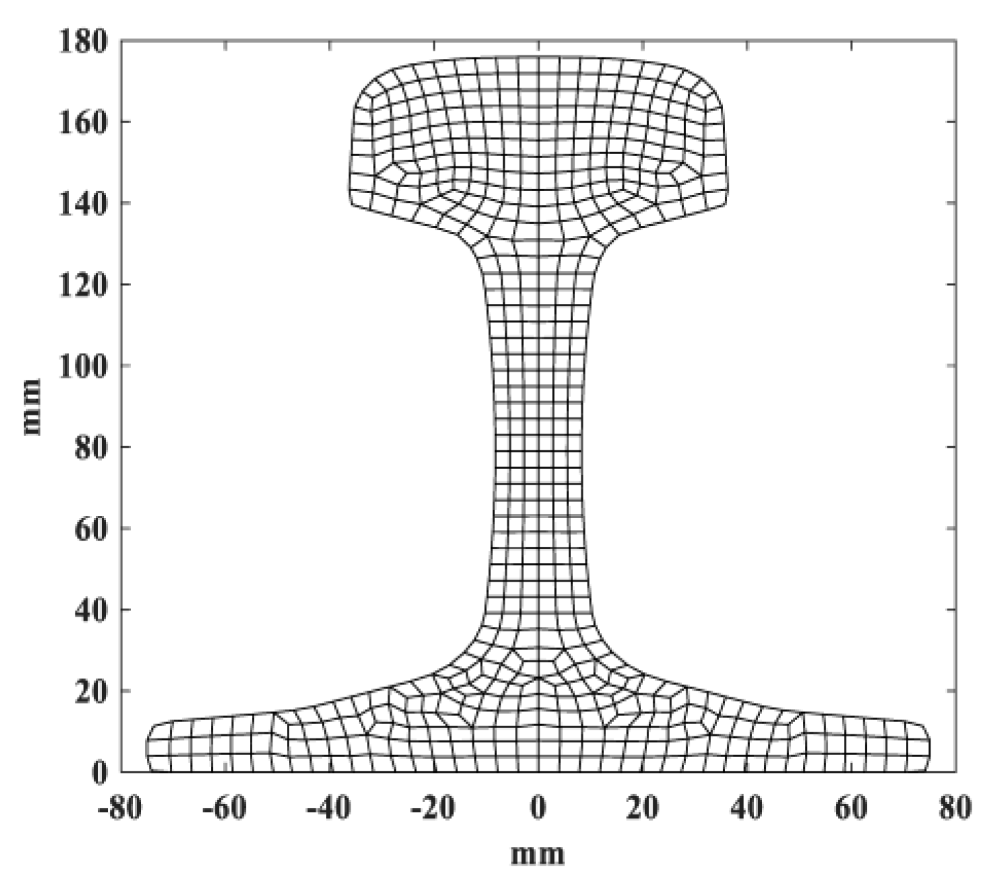
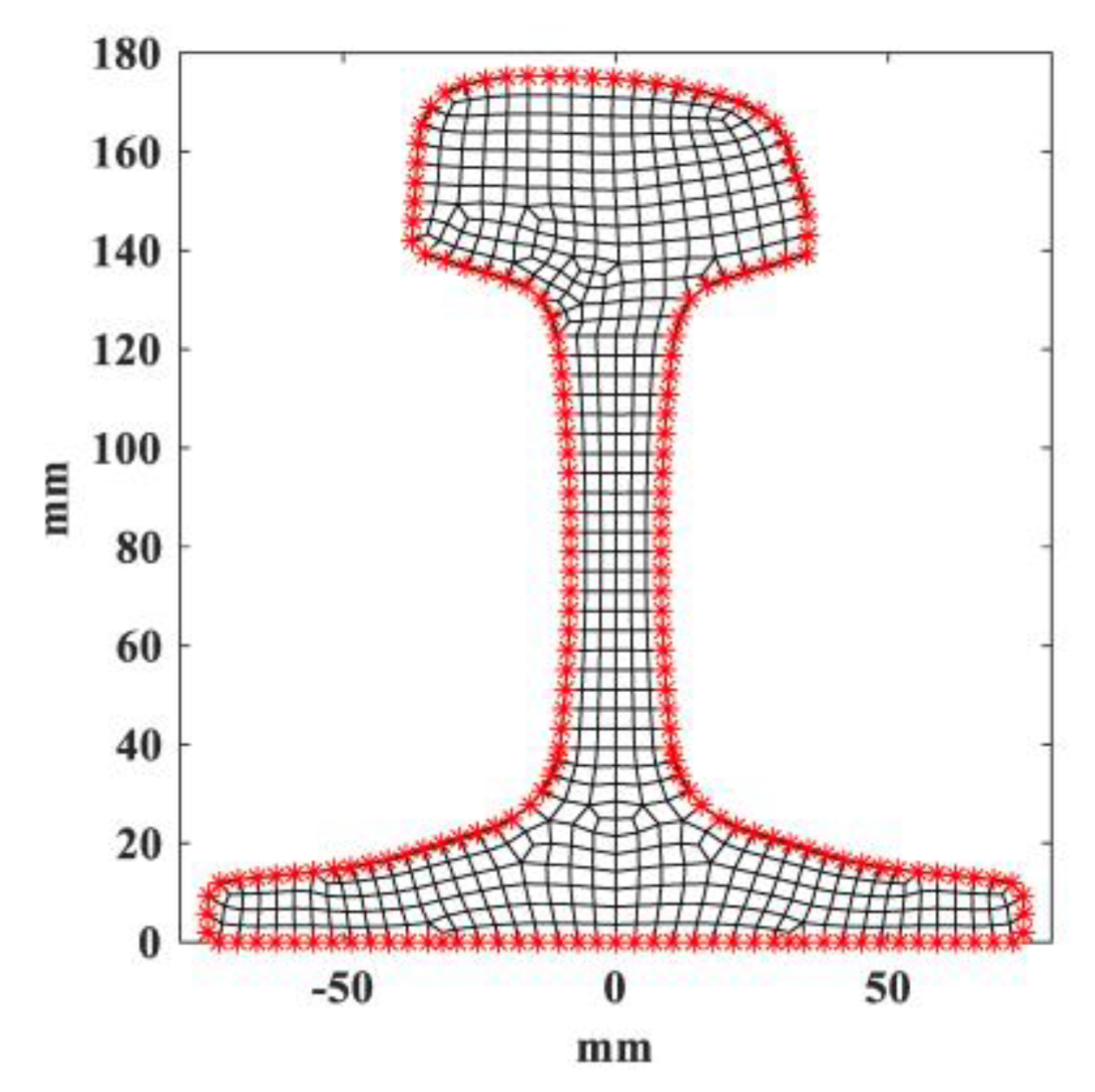
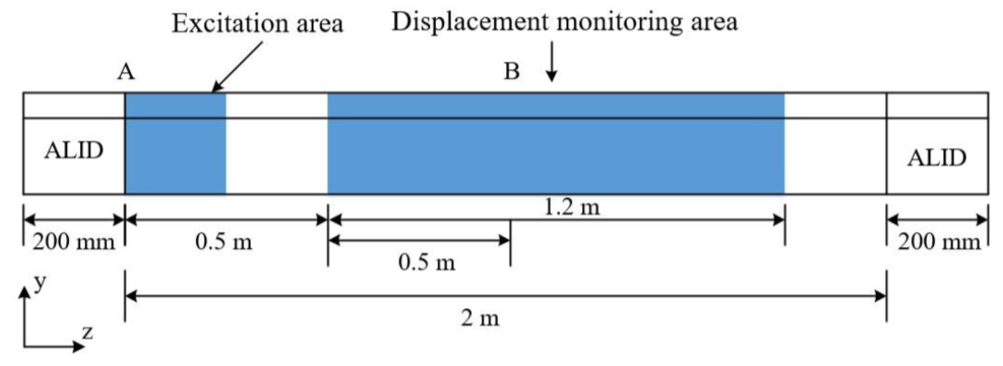
4.1. Three-Dimensional Finite Element Model of Continuously Welded Rail
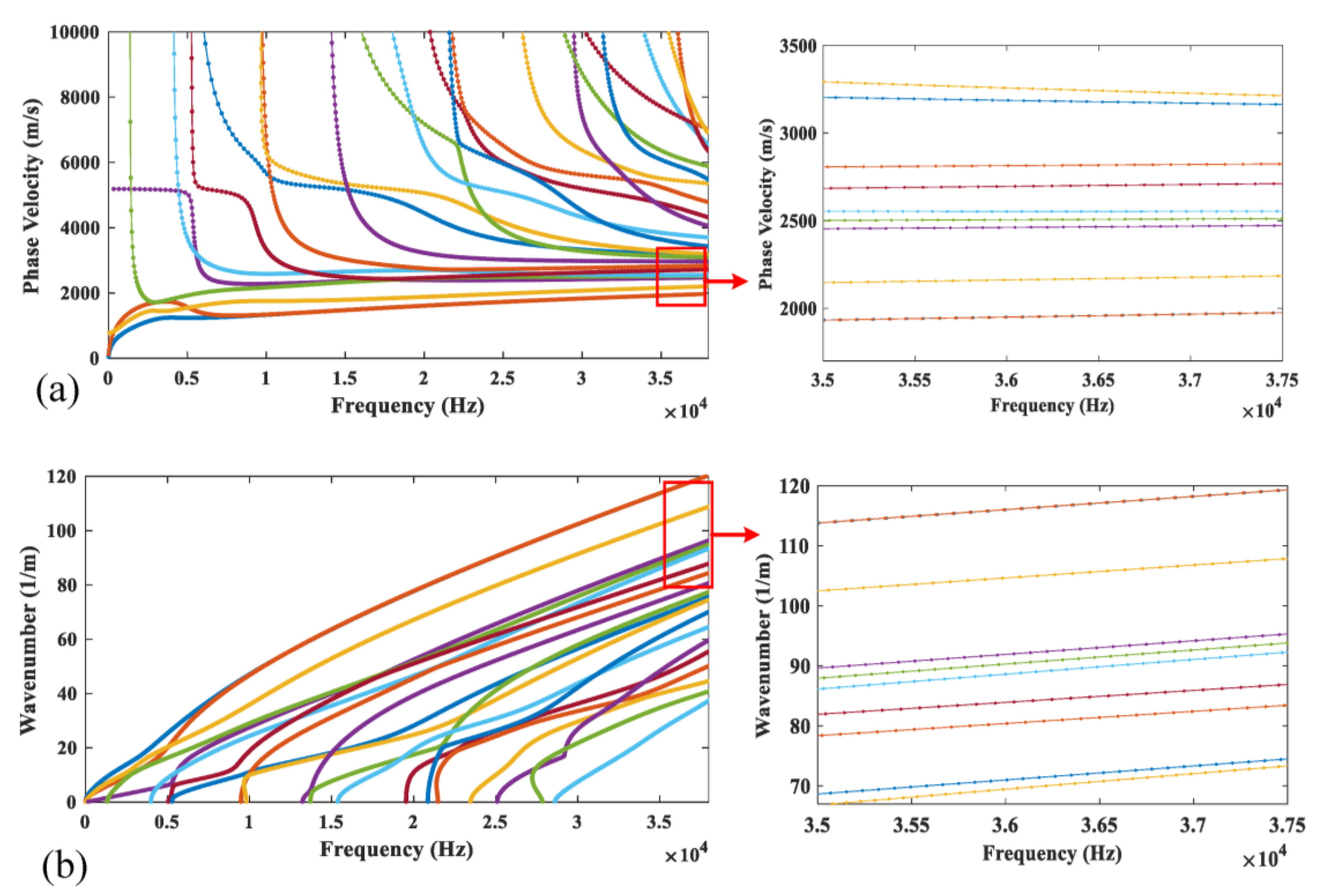
4.2. Finite Element Analysis Results
4.3. Identification of Material Properties Based on the FEM Simulation
5. Discussions and Conclusions
Author Contributions
Funding
Conflicts of Interest
References
- Kundu, T.; Loveday, P.W.; Wilcox, P.D. Guided wave propagation as a measure of axial loads in rails. Proc. SPIE 2010, 7650, 765023. [Google Scholar]
- Vishnuvardhan, J.; Krishnamurthy, C.V.; Balasubramaniam, K. Genetic algorithm based reconstruction of the elastic moduli of orthotropic plates using an ultrasonic guided wave single-transmitter-multiple-receiver SHM array. Smart Mater. Struct. 2007, 16, 1639–1650. [Google Scholar] [CrossRef]
- Sale, M.; Rizzo, P.; Marzani, A. Semi-analytical formulation for the guided waves-based reconstruction of elastic moduli. Mech Syst Signal. Pr. 2011, 25, 2241–2256. [Google Scholar] [CrossRef]
- Pabisek, E.; Waszczyszyn, Z. Identification of thin elastic isotropic plate parameters applying Guided Wave Measurement and Artificial Neural Networks. Mech. Syst. Signal. Process. 2015, 64–65, 403–412. [Google Scholar] [CrossRef]
- Rogers, W. Elastic property measurement using Rayleigh-Lamb waves. Res. Nondestruct. Eval. 1995, 6, 185–208. [Google Scholar] [CrossRef]
- Ambrozinski, L.; Packo, P.; Pieczonka, L.; Stepinski, T.; Uhl, T.; Staszewski, W.J. Identification of material properties - efficient modelling approach based on guided wave propagation and spatial multiple signal classification. Struct. Control. Health Monit. 2015, 22, 969–983. [Google Scholar] [CrossRef]
- Webersen, M.; Johannesmann, S.; Düchting, J.; Claes, L.; Henning, B. Guided ultrasonic waves for determining effective orthotropic material parameters of continuous-fiber reinforced thermoplastic plates. Ultrasonics 2018, 84, 53–62. [Google Scholar] [CrossRef]
- Rao, N.S. Inverse Problems in Ultrasonic Non-Destructive Characterization of Composite Materials Using Genetic Algorithms. MSc. Thesis, Aerospace Engineering, Misissippi State University, Starkville, MI, USA, 1997. [Google Scholar]
- Eremin, A.; Glushkov, E.; Glushkova, N.; Lammering, R. Evaluation of effective elastic properties of layered composite fiber-reinforced plastic plates by piezoelectrically induced guided waves and laser Doppler vibrometry. Compos. Struct 2015, 125, 449–458. [Google Scholar] [CrossRef]
- Bochud, N.; Laurent, J.; Bruno, F.; Royer, D.; Prada, C. Towards real-time assessment of anisotropic plate properties using elastic guided waves. J. Acoust. Soc. Am. 2018, 143, 1138–1147. [Google Scholar] [CrossRef]
- Rokhlin, S.; Chimenti, D.E. Reconstruction of elastic constants from ultrasonic reflectivity data in a fluid coupled composite plate. In Review of Progress in Quantitative Nondestructive Evaluation; Springer: Berlin/Heidelberg, Germany, 1990. [Google Scholar]
- Liu, G.; Han, X.; Lam, K. Material characterization of FGM plates using elastic waves and an inverse procedure. J. Compos. Mater. 2001, 35, 954–971. [Google Scholar] [CrossRef]
- Liu, G.; Ma, W.; Han, X. An inverse procedure for determination of material constants of composite laminates using elastic waves. Comput. Methods Appl. Mech. Eng. 2002, 191, 3543–3554. [Google Scholar] [CrossRef]
- Karim, M.R.; Mal, A.; Bar-Cohen, Y. Inversion of leaky Lamb wave data by simplex algorithm. J. Acoust. Soc. Am. 1990, 88, 482–491. [Google Scholar] [CrossRef]
- Cui, R.; Lanza di Scalea, F. On the identification of the elastic properties of composites by ultrasonic guided waves and optimization algorithm. Compos. Struct. 2019, 223, 110969. [Google Scholar] [CrossRef]
- Yu, J.; Wu, B. The inverse of material properties of functionally graded pipes using the dispersion of guided waves and an artificial neural network. Ndt E Int. 2009, 42, 452–458. [Google Scholar] [CrossRef]
- Setshedi, I.I.; Loveday, P.W.; Long, C.S.; Wilke, D.N. Estimation of rail properties using semi-analytical finite element models and guided wave ultrasound measurements. Ultrasonics 2019, 96, 240–252. [Google Scholar] [CrossRef] [PubMed]
- Hayashi, T.; Song, W.-J.; Rose, J.L. Guided wave dispersion curves for a bar with an arbitrary cross-section, a rod and rail example. Ultrasonics 2003, 41, 175–183. [Google Scholar] [CrossRef]
- Hayashi, T.; Tamayama, C.; Murase, M. Wave structure analysis of guided waves in a bar with an arbitrary cross-section. Ultrasonics 2006, 44, 17–24. [Google Scholar] [CrossRef]
- Bartoli, I.; Marzani, A.; di Scalea, F.L.; Viola, E. Modeling wave propagation in damped waveguides of arbitrary cross-section. J. Sound Vib. 2006, 295, 685–707. [Google Scholar] [CrossRef]
- Loveday, P.W. Semi-analytical finite element analysis of elastic waveguides subjected to axial loads. Ultrasonics 2009, 49, 298–300. [Google Scholar] [CrossRef]
- Gavrić, L. Computation of propagative waves in free rail using a finite element technique. J. Sound Vib. 1995, 185, 531–543. [Google Scholar] [CrossRef]
- Duan, X.; Yu, Z.; Zhu, L.; Xu, X. Monitoring system of thermal stress for continuous welded rails. Wit Trans. Built Env. 2016, 162, 239–249. [Google Scholar]
- Duan, X.; Yu, Z.; Zhu, L.; Xu, X. The Verification of Rail Thermal Stress Measurement System. Period. Polytech. Transp. Eng. 2017, 48, 45–51. [Google Scholar]
- Timoshenko, S.; Timoshenko, S.; Goodier, J. Theory of Elasticity; Timoshenko, S., Goodier, J.N., Eds.; McGraw-Hill book Company: New York, NY, USA, 1951. [Google Scholar]
- Belen’kiĭ, G.L.; Salaev, É.Y.; Suleĭmanov, R.A. Deformation effects in layer crystals. Uspekhi Fiz. Nauk 2007, 31, 434. [Google Scholar]
- Hooke, R. De Potentia Restitutiva, or of Spring Explaining the Power of Springing Bodies (Sixth Cutler Lecture, published in 1678). Rt Gunther Facsim. Repr. Early Sci. Oxf. Lond. Dawson Pall Mall 1968, 1969, 331–356. [Google Scholar]
- Sachse, W.; Pao, Y.H. On the determination of phase and group velocities of dispersive waves in solids. J. Appl. Phys. 1978, 49, 4320–4327. [Google Scholar] [CrossRef]
- Alleyne, D.; Cawley, P. A two-dimensional Fourier transform method for the measurement of propagating multimode signals. J. Acoust. Soc. Am. 1991, 89, 1159–1168. [Google Scholar] [CrossRef]
- Oran Brigham, E. The Fast Fourier Transform and its Applications; UK: Prentice Hall: Upper Saddle River, NJ, USA, 1988. [Google Scholar]
- Baker, J.E. Adaptive selection methods for genetic algorithms. In Proceedings of the International Conference on Genetic Algorithms and their applications, Pittsburgh, PA, USA, 24–26 July 1985; Hillsdale: New Jersey, NJ, USA, 1985; pp. 101–111. [Google Scholar]
- Srinivas, M.; Patnaik, L.M. Adaptive probabilities of crossover and mutation in genetic algorithms. IEEE Trans. Syst. Mancybern. 1994, 24, 656–667. [Google Scholar] [CrossRef]
- Capelli, F.; Riba, J.-R.; Rupérez, E.; Sanllehí, J. A Genetic-Algorithm-Optimized Fractal Model to Predict the Constriction Resistance From Surface Roughness Measurements. IEEE Trans. Instrum. Meas. 2017, 66, 2437–2447. [Google Scholar] [CrossRef]
- Wardeh, M.A.; Toutanji, H.A. Parameter estimation of an anisotropic damage model for concrete using genetic algorithms. Int. J. Damage Mech. 2017, 26, 801–825. [Google Scholar] [CrossRef]
- Duan, X.; Zhu, L.; Yu, Z.; Xu, X. Estimating the Axial Load of In-Service Continuously Welded Rail Under the Influences of Rail Wear and Temperature. IEEE Access 2019, 7, 143524–143538. [Google Scholar] [CrossRef]
- Railways, C.M. Railway Line Repair Regulations. 2006. [Google Scholar]
- Xu, X.; Zhuang, L.; Xing, B.; Yu, Z.; Zhu, L. An Ultrasonic Guided Wave Mode Excitation Method in Rails. IEEE Access 2018, 6, 60414–60428. [Google Scholar]
- Xuan, G. An Euclidean Distance Feature Selection Method in Pattern Recognition. Comput. Appl. Softw. 1985, 6. [Google Scholar]
- Rose, J.; Pelts, S.; Quarry, M. A comb transducer model for guided wave NDE. Ultrasonics 1998, 36, 163–169. [Google Scholar] [CrossRef]
- Bartoli, I.; di Scalea, F.L.; Fateh, M.; Viola, E. Modeling guided wave propagation with application to the long-range defect detection in railroad tracks. Ndt E Int. 2005, 38, 325–334. [Google Scholar] [CrossRef]
- Moser, F.; Jacobs, L.J.; Qu, J. Modeling elastic wave propagation in waveguides with the finite element method. Ndt E Int. 1999, 32, 225–234. [Google Scholar] [CrossRef]
- Fellinger, P.; Marklein, R.; Langenberg, K.J.; Klaholz, S. Numerical modeling of elastic wave propagation and scattering with EFIT—elastodynamic finite integration technique. Wave Motion 1995, 21, 47–66. [Google Scholar] [CrossRef]
- Drozdz, M.; Skelton, E.; Craster, R.; Lowe, M. Modeling bulk and guided waves in unbounded elastic media using absorbing layers in commercial finite element packages. In AIP Conference Proceedings; AIP: Melville, SNY, USA, 2017; pp. 87–94. [Google Scholar]
- Rajagopal, P.; Drozdz, M.; Skelton, E.A.; Lowe, M.J.; Craster, R.V. On the use of absorbing layers to simulate the propagation of elastic waves in unbounded isotropic media using commercially available finite element packages. Ndt E Int. 2012, 51, 30–40. [Google Scholar] [CrossRef]
- Moreau, L.; Velichko, A.; Wilcox, P. Accurate finite element modelling of guided wave scattering from irregular defects. Ndt E Int. 2012, 45, 46–54. [Google Scholar] [CrossRef]


| Parameters | Settings |
|---|---|
| Size of Population | 10 |
| Max Generations | 20 |
| Selection | Stochastic Universal Sampling and Elitist Preservation |
| Crossover | Arithmetic crossover |
| Mutation | Uniform mutation |
| Probability of Crossover | |
| Probability of Mutation |
| Mode number | = 212 GPa | = 216 GPa | |
|---|---|---|---|
| 1 | 1953.916 | 1969.959 | 16.043 |
| 2 | 1956.276 | 1972.344 | 16.067 |
| 3 | 2205.867 | 2225.191 | 19.324 |
| 4 | 2517.632 | 2544.668 | 27.036 |
| 5 | 2580.399 | 2609.510 | 29.111 |
| 6 | 2651.980 | 2684.784 | 32.805 |
| 7 | 2659.204 | 2686.379 | 27.175 |
| 8 | 2816.061 | 2846.475 | 30.414 |
| 9 | 2970.044 | 3006.502 | 36.458 |
| 10 | 3173.780 | 3222.459 | 48.679 |
| Mode Number | = 84.0 GPa | = 81.4 GPa | |
|---|---|---|---|
| 1 | 1936.983 | 1933.119 | 3.864 |
| 2 | 1937.294 | 1933.419 | 3.875 |
| 3 | 2143.746 | 2145.276 | 1.530 |
| 4 | 2463.301 | 2455.438 | 7.863 |
| 5 | 2506.153 | 2501.901 | 4.252 |
| 6 | 2562.416 | 2554.812 | 7.604 |
| 7 | 2711.886 | 2689.929 | 21.957 |
| 8 | 2831.896 | 2811.611 | 20.285 |
| 9 | 2999.006 | 2967.924 | 31.082 |
| 10 | 3152.497 | 3124.218 | 28.278 |
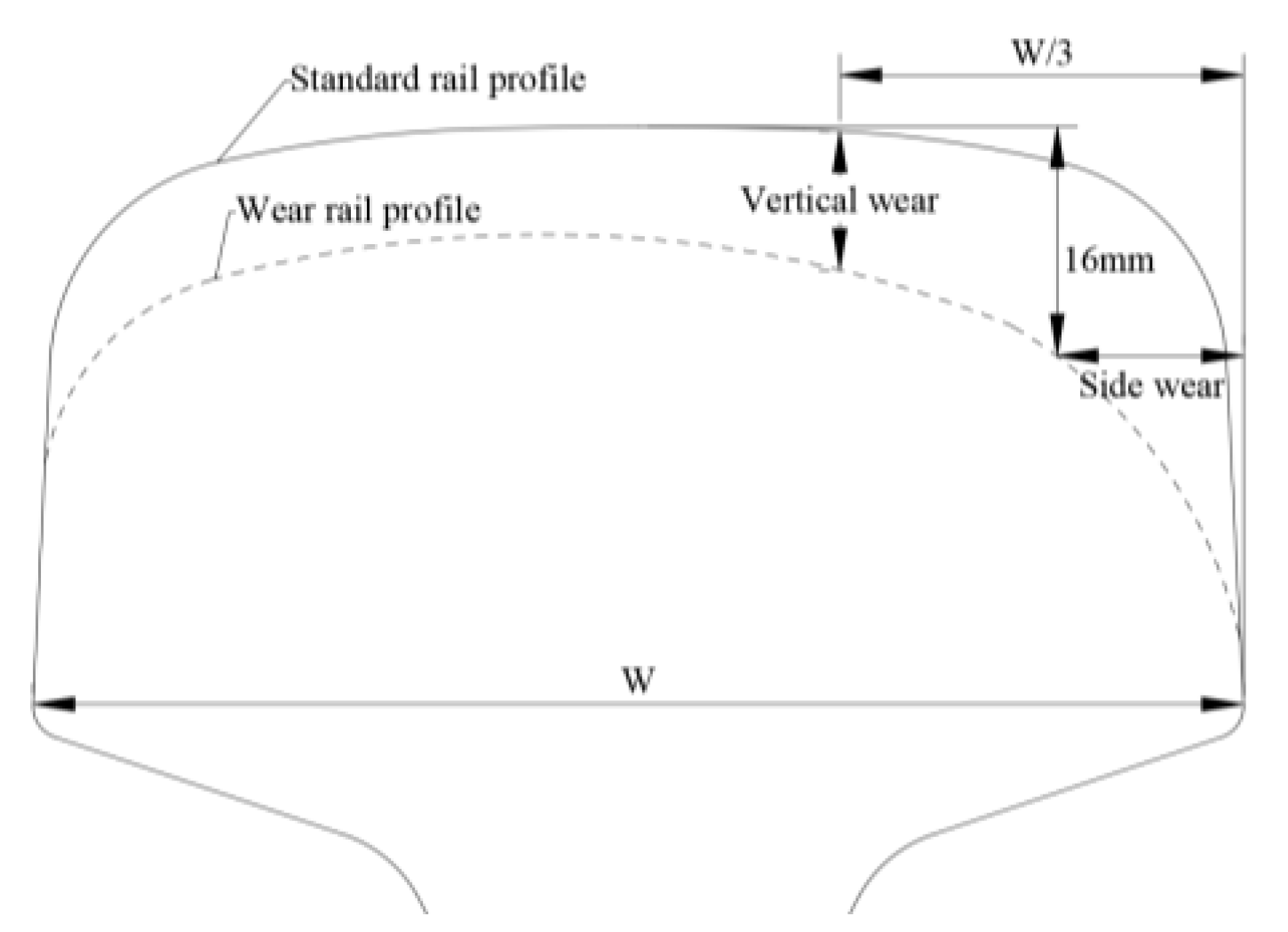
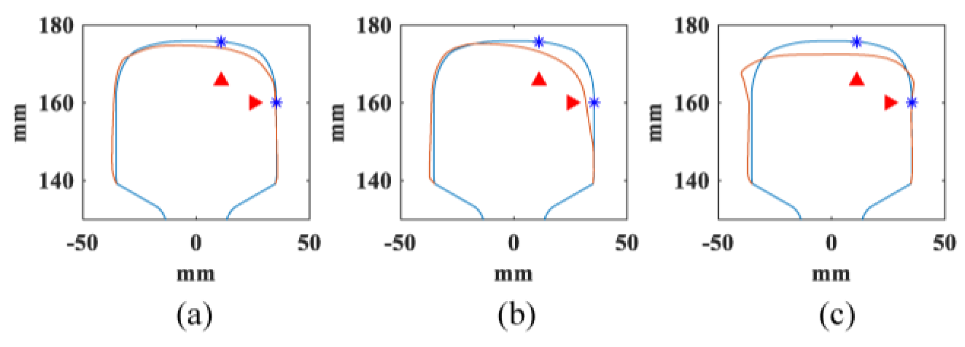
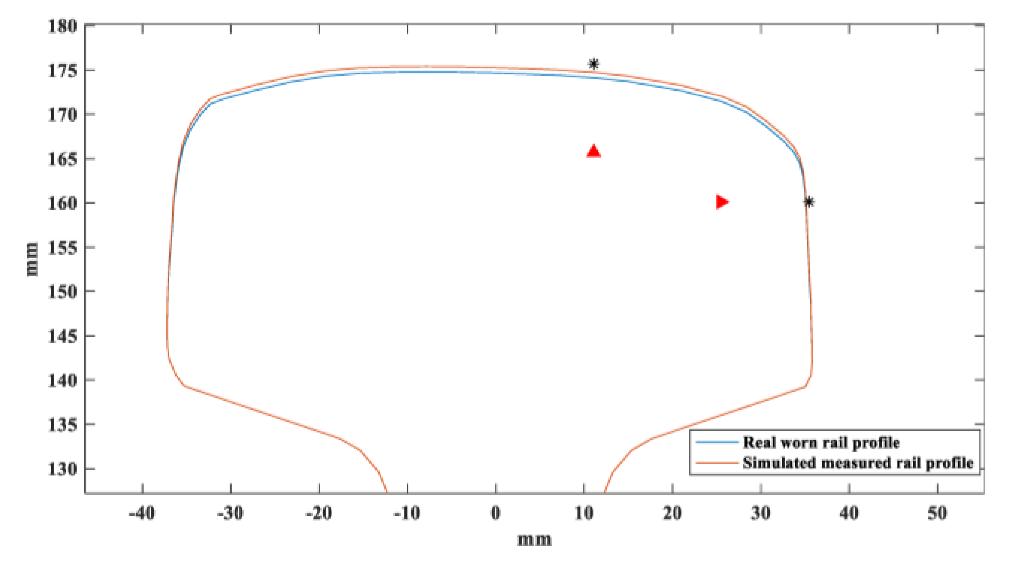
| Profile Number | Vertical Wear | Side Wear | Total Wear |
|---|---|---|---|
| a | 1.50 mm | 0.39 mm | 1.70 mm |
| b | 2.50 mm | 3.66 mm | 4.33 mm |
| c | 6.00 mm | 5.43 mm | 8.72 mm |
| Mode number | Profile a | (in percent) | Profile b | (in percent) | Profile c | (in percent) |
|---|---|---|---|---|---|---|
| 1 | 1951.8007 | 0.2115 | 1951.8007 | 0.2115 | 1951.8007 | 0.2115 |
| 2 | 1952.0716 | 0.2116 | 1952.0716 | 0.2116 | 1952.0716 | 0.2116 |
| 3 | 2171.8942 | 0.1184 | 2171.8911 | 0.1183 | 2171.9765 | 0.1222 |
| 7 | 2688.0976 | 0.6833 | 2689.5073 | 0.6312 | 2651.4328 | 2.0380 |
| 9 | 2957.0585 | 0.5539 | 2967.3489 | 0.2087 | 2926.0728 | 1.5960 |
| 10 | 3112.6723 | 0.2611 | 3116.1250 | 0.1504 | 3108.9001 | 0.3819 |
| Mode number | Profile a | (in percent) | Profile b | (in percent) | Profile c | (in percent) |
|---|---|---|---|---|---|---|
| 1 | 115.8902 | 0.2119 | 115.8902 | 0.2119 | 115.8902 | 0.2119 |
| 2 | 115.8742 | 0.2121 | 115.8742 | 0.2121 | 115.8742 | 0.2121 |
| 3 | 104.1463 | 0.1183 | 104.1464 | 0.1181 | 104.1423 | 0.1220 |
| 7 | 84.1467 | 0.6880 | 84.1026 | 0.6352 | 85.3104 | 2.0804 |
| 9 | 76.4931 | 0.5570 | 76.2279 | 0.2083 | 77.3032 | 1.6218 |
| 10 | 72.6690 | 0.2617 | 72.5884 | 0.1506 | 72.7571 | 0.3834 |
| Mode 1 | Mode 2 | Mode 3 | |
|---|---|---|---|
| Nodes | 364, 602 | 364, 602 | 674 |
| Direction | axis negative | axis positive and negative | axis negative |
| Excitation Type | Two-sided symmetric excitation | Two-sided anti-symmetric excitation | Single point excitation |
| Mode 7 | Mode 9 | Mode 10 | |
|---|---|---|---|
| Nodes | 198, 233 / 210, 220 | 231, 342, 674, 251 / 200, 624, 261, 684 | 603, 266, 679, 202 / 363, 669, 256, 229 |
| Direction | axis positive and negative | axis positive and negative | axis positive and negative |
| Excitation Type | Four points excitation | Two-sided eight points anti-symmetric excitation | Two-sided eight points anti-symmetric excitation |
| Rail Profile | a | b | c |
|---|---|---|---|
| expected value | 215.0000 | 213.0000 | 214.0000 |
| estimated value | 213.4162 | 211.7086 | 214.2204 |
| Relative error | 0.6918 | 0.6063 | 0.1030 |
| Standard deviation | 0.0281 | 0.2852 | 0.3102 |
| expected value | 79.6296 | 81.9231 | 83.5938 |
| estimated value | 77.0549 | 79.3510 | 81.8056 |
| Relative error | 2.5748 | 3.1397 | 2.1391 |
| Standard deviation | 0.1325 | 0.1950 | 0.7457 |
| Rail Profile | a | b | c |
|---|---|---|---|
| E expected value | 215.0000 | 213.0000 | 214.0000 |
| E estimated value | 215.1166 | 212.2261 | 213.7712 |
| Relative error | 0.0542 | 0.3633 | 0.1069 |
| Standard deviation σ | 0.0790 | 0.1502 | 0.2009 |
| G expected value | 79.6296 | 81.9231 | 83.5938 |
| G estimated value | 79.6635 | 81.4885 | 84.3168 |
| Relative error | 0.0339 | 0.5183 | 0.8649 |
| Standard deviation σ | 0.0425 | 0.2447 | 0.1858 |
| Rail Profile | a | b | c |
|---|---|---|---|
| expected value | 215.0000 | 213.0000 | 214.0000 |
| estimated value | 213.0220 | 215.5720 | 217.7630 |
| Relative error | 0.9200 | 1.2075 | 1.7584 |
| Standard deviation | 0.0879 | 0.2060 | 0.1702 |
| expected value | 79.6296 | 81.9231 | 83.5938 |
| estimated value | 72.9987 | 74.4484 | 75.6311 |
| Relative error | 8.3272 | 9.1240 | 9.5254 |
| Standard deviation | 0.1931 | 0.8450 | 0.5368 |
| Rail Profile | a | b | c |
|---|---|---|---|
| expected value | 215.0000 | 213.0000 | 214.0000 |
| estimated value | 213.6946 | 211.6890 | 215.0104 |
| Relative error | 0.6072 | 0.6155 | 0.4721 |
| Standard deviation | 0.1163 | 0.0922 | 0.2090 |
| expected value | 79.6296 | 81.9231 | 83.5938 |
| estimated value | 73.2284 | 78.0646 | 74.8453 |
| Relative error | 8.0388 | 4.7099 | 10.4654 |
| Standard deviation | 0.8046 | 0.1264 | 0.6393 |
© 2020 by the authors. Licensee MDPI, Basel, Switzerland. This article is an open access article distributed under the terms and conditions of the Creative Commons Attribution (CC BY) license (http://creativecommons.org/licenses/by/4.0/).
Share and Cite
Zhu, L.; Duan, X.; Yu, Z. On the Identification of Elastic Moduli of In-Service Rail by Ultrasonic Guided Waves. Sensors 2020, 20, 1769. https://doi.org/10.3390/s20061769
Zhu L, Duan X, Yu Z. On the Identification of Elastic Moduli of In-Service Rail by Ultrasonic Guided Waves. Sensors. 2020; 20(6):1769. https://doi.org/10.3390/s20061769
Chicago/Turabian StyleZhu, Liqiang, Xiangyu Duan, and Zujun Yu. 2020. "On the Identification of Elastic Moduli of In-Service Rail by Ultrasonic Guided Waves" Sensors 20, no. 6: 1769. https://doi.org/10.3390/s20061769
APA StyleZhu, L., Duan, X., & Yu, Z. (2020). On the Identification of Elastic Moduli of In-Service Rail by Ultrasonic Guided Waves. Sensors, 20(6), 1769. https://doi.org/10.3390/s20061769