Visual Analysis of Odor Interaction Based on Support Vector Regression Method


Abstract
1. Introduction
2. Materials and Methods
2.1. Stimuli and Odor Data
2.2. Support Vector Regression Methodology
2.3. Experimental Procedure
3. Results and Discussion
3.1. Odor Intensity Predictive Performance of the SVR Model
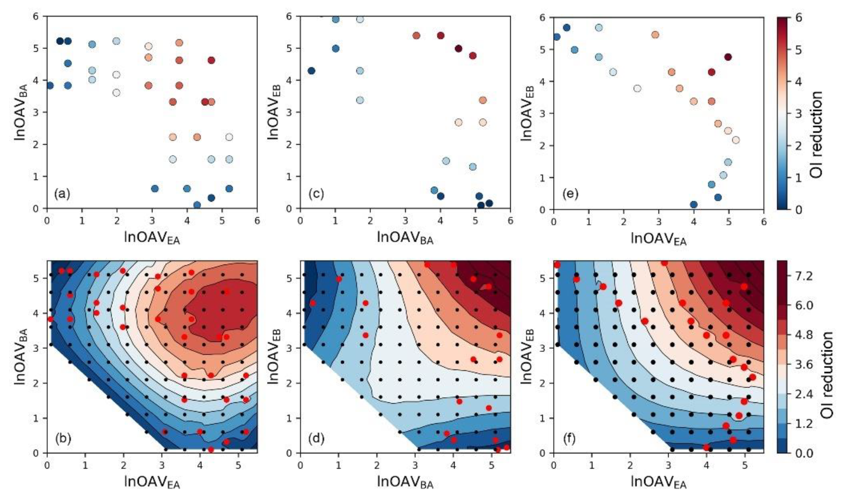
3.2. SVR-Assisted Visual Analysis of Odor Interaction
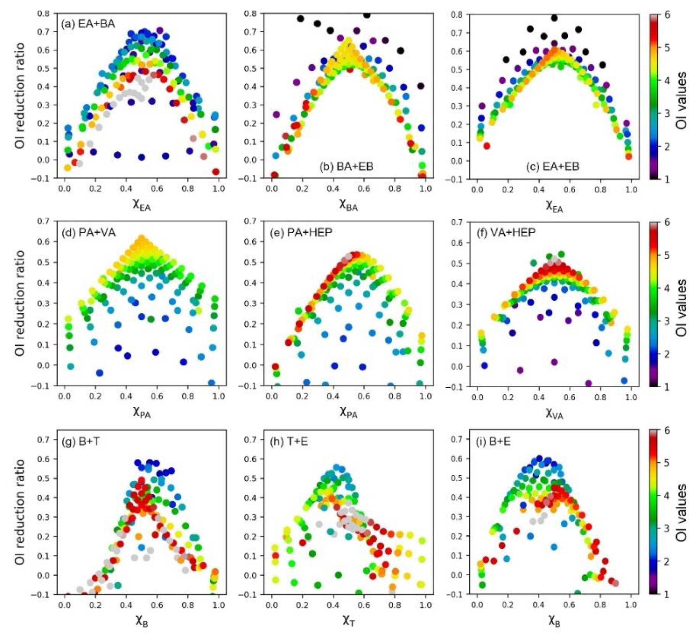
3.3. Similarity of Binary Odor Interaction Pattern
4. Conclusions
Supplementary Materials
Author Contributions
Funding
Conflicts of Interest
References
- Jiang, G.M.; Melder, D.; Keller, J.; Yuan, Z.G. Odor emissions from domestic wastewater: A review. Crit. Rev. Environ. Sci. Technol. 2017, 47, 1581–1611. [Google Scholar] [CrossRef]
- Le Berre, E.; Beno, N.; Ishii, A.; Chabanet, C.; Etievant, P.; Thomas-Danguin, T. Just noticeable differences in component concentrations modify the odor quality of a blending mixture. Chem. Senses 2008, 33, 389–395. [Google Scholar] [CrossRef] [PubMed]
- Lewkowska, P.; Dymerski, T.; Gebicki, J.; Namiesnik, J. The use of sensory analysis techniques to assess the quality of indoor air. Crit. Rev. Anal. Chem. 2017, 47, 37–50. [Google Scholar] [CrossRef] [PubMed]
- Atanasova, B.; Langlois, D.; Nicklaus, S.; Chabanet, C.; Etievant, P. Evaluation of olfactory intensity: Comparative study of two methods. J. Sens. Stud. 2004, 19, 307–326. [Google Scholar] [CrossRef]
- Wu, C.D.; Liu, J.M.; Zhao, P.; Piringer, M.; Schauberger, G. Conversion of the chemical concentration of odorous mixtures into odour concentration and odour intensity: A comparison of methods. Atmos. Environ. 2016, 127, 283–292. [Google Scholar] [CrossRef]
- Wakayama, H.; Sakasai, M.; Yoshikawa, K.; Inoue, M. Method for predicting odor intensity of perfumery raw materials using dse-response curve database. Ind. Eng. Chem. Res. 2019, 58, 15036–15044. [Google Scholar] [CrossRef]
- Sarkar, U.; Hobbs, S.E. Odour from municipal solid waste (MSW) landfills: A study on the analysis of perception. Environ. Int. 2002, 27, 655–662. [Google Scholar] [CrossRef]
- Yan, L.C.; Liu, J.M.; Wang, G.H.; Wu, C.D. An odor interaction model of binary odorant mixtures by a partial differential equation method. Sensors 2014, 14, 12256–12270. [Google Scholar] [CrossRef]
- Cain, W.S.; Schiet, F.T.; Olsson, M.J.; deWijk, R.A. Comparison of models of odor interaction. Chem. Senses 1995, 20, 625–637. [Google Scholar] [CrossRef]
- Olsson, M.J. An integrated model of intensity and quality of odor mixtures. Ann. N. Y. Acad. Sci. 1998, 855, 837–840. [Google Scholar] [CrossRef]
- Teixeira, M.A.; Rodriguez, O.; Rodrigues, A.E. The perception of fragrance mixtures: A comparison of odor intensity models. AIChE J. 2010, 56, 1090–1106. [Google Scholar] [CrossRef]
- Yu, Z.M.; Guo, H.Q.; Lague, C. Development of a livestock odor dispersion model: Part II. Evaluation and validation. J. Air Waste Manag. 2011, 61, 277–284. [Google Scholar] [CrossRef] [PubMed][Green Version]
- Schiffman, S.S.; McLaughlin, B.; Katul, G.G.; Nagle, H.T. Eulerian-Lagrangian model for predicting odor dispersion using instrumental and human measurements. Sens. Actuat. B Chem. 2005, 106, 122–127. [Google Scholar] [CrossRef]
- Olsson, M.J. An interaction-model for odor quality and intensity. Percept. Psychophys. 1994, 55, 363–372. [Google Scholar] [CrossRef] [PubMed]
- Teixeira, M.A.; Rodriguez, O.; Rodrigues, A.E. Prediction model for the odor intensity of fragrance mixtures: A valuable tool for perfumed product design. Ind. Eng. Chem. Res. 2013, 52, 963–971. [Google Scholar] [CrossRef]
- Butler, K.T.; Davies, D.W.; Cartwright, H.; Isayev, O.; Walsh, A. Machine learning for molecular and materials science. Nature 2018, 559, 547–555. [Google Scholar] [CrossRef]
- Vu, T.V.; Shi, Z.B.; Cheng, J.; Zhang, Q.; He, K.B.; Wang, S.X.; Harrison, R.M. Assessing the impact of clean air action on air quality trends in Beijing using a machine learning technique. Atmos. Chem. Phys. 2019, 19, 11303–11314. [Google Scholar] [CrossRef]
- Arabgol, R.; Sartaj, M.; Asghari, K. Predicting nitrate concentration and its spatial distribution in groundwater resources using support vector machines (SVMs) model. Environ. Model. Assess. 2016, 21, 71–82. [Google Scholar] [CrossRef]
- Vega García, M.; Aznarte, J.L. Shapley additive explanations for NO2 forecasting. Ecol. Inform. 2020, 56, 101039. [Google Scholar] [CrossRef]
- Vanarse, A.; Osseiran, A.; Rassau, A. Real-time classification of multivariate olfaction data using spiking neural networks. Sensors 2019, 19, 1841. [Google Scholar] [CrossRef]
- Szulczynski, B.; Gebicki, J. Determination of odor intensity of binary gas mixtures using perceptual models and an electronic nose combined with fuzzy logic. Sensors 2019, 19, 3473. [Google Scholar] [CrossRef]
- Zhu, L.T.; Jia, H.L.; Chen, Y.B.; Wang, Q.; Li, M.W.; Huang, D.Y.; Bai, Y.L. A novel method for soil organic matter determination by using an artificial olfactory system. Sensors 2019, 19, 3417. [Google Scholar] [CrossRef] [PubMed]
- Yan, L.C.; Liu, J.M.; Jiang, S.; Wu, C.D.; Gao, K.W. The regular interaction pattern among odorants of the same type and its application in odor intensity assessment. Sensors 2017, 17, 1624. [Google Scholar] [CrossRef]
- Yan, L.C.; Liu, J.M.; Fang, D. Use of a modified vector model for odor intensity prediction of odorant mixtures. Sensors 2015, 15, 5697–5709. [Google Scholar] [CrossRef]
- Yan, L.C.; Liu, J.M.; Qu, C.; Gu, X.Y.; Zhao, X. Research on odor interaction between aldehyde compounds via a partial differential equation (PDE) model. Sensors 2015, 15, 2888–2901. [Google Scholar]
- Krajewski, S.; Nowacki, J. Dual-phase steels microstructure and properties consideration based on artificial intelligence techniques. Arch. Civ. Mech. Eng. 2014, 14, 278–286. [Google Scholar] [CrossRef]
- Mariette, A.; Rahul, K. Efficient Learning Machines, 1st ed.; Apress: New York, NY, USA, 2015; p. 67. [Google Scholar]
- Wen, Y.F.; Cai, C.Z.; Liu, X.H.; Pei, J.F.; Zhu, X.J.; Xiao, T.T. Corrosion rate prediction of 3C steel under different seawater environment by using support vector regression. Corros. Sci. 2009, 51, 349–355. [Google Scholar] [CrossRef]
- Azimi, H.; Bonakdari, H.; Ebtehaj, I. Design of radial basis function-based support vector regression in predicting the discharge coefficient of a side weir in a trapezoidal channel. Appl. Water Sci. 2019, 9, 78. [Google Scholar] [CrossRef]
- Shi, H.; Xiao, H.; Zhou, J.; Li, N.; Zhou, H. Radial basis function kernel parameter optimization algorithm in support vector machine based on segmented dichotomy. In Proceedings of the 5th International Conference on Systems and Informatics (ICSAI), Nanjing, China, 10–12 November 2018; pp. 383–388. [Google Scholar]
- Laref, R.; Losson, E.; Sava, A.; Siadat, M. Support vector machine regression for calibration transfer between electronic noses dedicated to air pollution monitoring. Sensors 2018, 18, 3716. [Google Scholar] [CrossRef] [PubMed]
- Shin, D.; Yamamoto, Y.; Brady, M.P.; Lee, S.; Haynes, J.A. Modern data analytics approach to predict creep of high-temperature alloys. Acta Mater. 2019, 168, 321–330. [Google Scholar] [CrossRef]
- Sun, Y.T.; Bai, H.Y.; Li, M.Z.; Wang, W.H. Machine learning approach for prediction and understanding of glass-forming ability. J. Phys. Chem. Lett. 2017, 8, 3434–3439. [Google Scholar] [CrossRef] [PubMed]
- Kerckhoffs, J.; Hoek, G.; Portengen, L.; Brunekreef, B.; Vermeulen, R.C.H. Performance of prediction algorithms for modeling outdoor air pollution spatial surfaces. Environ. Sci. Technol. 2019, 53, 1413–1421. [Google Scholar] [CrossRef] [PubMed]
- Tsirikoglou, P.; Abraham, S.; Contino, F.; Lacor, C.; Ghorbaniasl, G. A hyperparameters selection technique for support vector regression models. Appl. Soft. Comput. 2017, 61, 139–148. [Google Scholar] [CrossRef]
- Brattoli, M.; de Gennaro, G.; de Pinto, V.; Loiotile, A.D.; Lovascio, S.; Penza, M. Odour detection methods: Olfactometry and chemical sensors. Sensors 2011, 11, 5290–5322. [Google Scholar] [CrossRef] [PubMed]
- Deshmukh, S.; Jana, A.; Bhattacharyya, N.; Bandyopadhyay, R.; Pandey, R.A. Quantitative determination of pulp and paper industry emissions and associated odor intensity in methyl mercaptan equivalent using electronic nose. Atmos. Environ. 2014, 82, 401–409. [Google Scholar] [CrossRef]
- Liu, T.P.; Zhang, W.T.; McLean, P.; Ueland, M.; Forbes, S.L.; Su, S.W. Electronic nose-based odor classification using genetic algorithms and fuzzy support vector machines. Int. J. Fuzzy Syst. 2018, 20, 1309–1320. [Google Scholar] [CrossRef]
- Pan, L.; Yang, S.X. An electronic nose network system for online monitoring of livestock farm odors. IEEE/ASME Trans. Mechatron. 2009, 14, 371–376. [Google Scholar] [CrossRef]
- Niu, Y.; Wang, P.; Xiao, Z.; Zhu, J.; Sun, X.; Wang, R. Evaluation of the perceptual interaction among ester aroma compounds in cherry wines by GC–MS, GC–O, odor threshold and sensory analysis: An insight at the molecular level. Food Chem. 2019, 275, 143–153. [Google Scholar] [CrossRef]
- Wu, Q.; Wang, Z.; Hu, X.; Zheng, T.; Yang, Z.; He, F.; Li, J.; Wang, J. Uncovering the eutectics design by machine learning in the Al–Co–Cr–Fe–Ni high entropy system. Acta Mater. 2020, 182, 278–286. [Google Scholar] [CrossRef]
- Chen, Z.Y.; Zhang, R.; Zhang, T.H.; Ou, C.Q.; Guo, Y. A kriging-calibrated machine learning method for estimating daily ground-level NO2 in mainland China. Sci. Total Environ. 2019, 690, 556–564. [Google Scholar] [CrossRef]
- Kim, K.H. Experimental demonstration of masking phenomena between competing odorants via an air dilution sensory test. Sensors 2010, 10, 7287–7302. [Google Scholar] [CrossRef] [PubMed]


| Order | Odorant (Abbreviation) | CAS# | Chemical Structure | Odor Threshold/mg/m3 |
|---|---|---|---|---|
| 1 | ethyl acetate (EA) | 141-78-6 |  | 0.276 I |
| 2 | butyl acetate (BA) | 123-86-4 |  | 0.085 I |
| 3 | ethyl butyrate (EB) | 105-54-4 |  | 0.053 I |
| 4 | propionaldehyde (PA) | 123-38-6 |  | 40.6 E-3 II |
| 5 | n-valeraldehyde (VA) | 110-62-3 |  | 20.5 E-3 II |
| 6 | n-heptaldehyde (HEP) | 117-71-7 |  | 26.0 E-3 II |
| 7 | benzene (B) | 71-43-2 |  | 2.53 III |
| 8 | toluene (T) | 108-88-3 |  | 1.43 III |
| 9 | Ethylbenzene (E) | 100-41-4 |  | 0.45 III |
| Mixture | R2 | MAE | ||
|---|---|---|---|---|
| Training Set | Test Set | Training Set | Test Set | |
| EA+BA | 0.97 | 0.95 | 0.15 | 0.26 |
| BA+EB | 0.96 | 0.85 | 0.15 | 0.33 |
| EA+EB | 0.87 | 0.87 | 0.17 | 0.25 |
| PA+VA | 0.95 | 0.78 | 0.14 | 0.25 |
| PA+HEP | 0.96 | 0.94 | 0.17 | 0.23 |
| VA+HEP | 0.97 | 0.87 | 0.15 | 0.31 |
| B+T | 0.87 | 0.81 | 0.33 | 0.43 |
| T+E | 0.78 | 0.68 | 0.31 | 0.40 |
| B+E | 0.98 | 0.94 | 0.09 | 0.27 |
© 2020 by the authors. Licensee MDPI, Basel, Switzerland. This article is an open access article distributed under the terms and conditions of the Creative Commons Attribution (CC BY) license (http://creativecommons.org/licenses/by/4.0/).
Share and Cite
Yan, L.; Wu, C.; Liu, J. Visual Analysis of Odor Interaction Based on Support Vector Regression Method. Sensors 2020, 20, 1707. https://doi.org/10.3390/s20061707
Yan L, Wu C, Liu J. Visual Analysis of Odor Interaction Based on Support Vector Regression Method. Sensors. 2020; 20(6):1707. https://doi.org/10.3390/s20061707
Chicago/Turabian StyleYan, Luchun, Chuandong Wu, and Jiemin Liu. 2020. "Visual Analysis of Odor Interaction Based on Support Vector Regression Method" Sensors 20, no. 6: 1707. https://doi.org/10.3390/s20061707
APA StyleYan, L., Wu, C., & Liu, J. (2020). Visual Analysis of Odor Interaction Based on Support Vector Regression Method. Sensors, 20(6), 1707. https://doi.org/10.3390/s20061707