Low Energy Consumption Compressed Spectrum Sensing Based on Channel Energy Reconstruction in Cognitive Radio Network


Abstract
1. Introduction
- No relay on prior information. The prior information of the spectrum signal does not need to be known in advance, and we only reconfigure the channel energy. Using the sparsity of the channel energy, a wideband filter bank is used to obtain a linear measurement of the channel energy, whose value is used to determine whether the channel is occupied. Compared with the previous algorithms, the proposed algorithm focuses on the direct recovery of the spectrum channel energy instead of the restoring of the entire spectrum signal. Hence, the data processing operation is lower during the sensing process.
- Low storage overhead and low sampling rate. Based on the compressed sensing theory, our algorithm can compress high-dimensional signals using low-dimensional sensing matrices. According to the characteristics of the semi-tensor product, fewer wideband filters for the proposed algorithm are required than traditional compressed spectrum sensing algorithms. Hence, the storage overhead of the CR node will be greatly reduced and the sensing process is more efficient.
- Parallel reconstruction and less time required. The reconstruction method of semi-tensor compressed spectrum sensing can be implemented in parallel. Based on the characteristics of the semi-tensor product, the channel energy is simultaneously performed in multiple compressed sensing (CS) decoders so that the total spectrum sensing time is markedly reduced, which provides an important contribution to the immediacy of dynamic spectrum access.
2. Fundamental Knowledge
2.1. Cognitive Radio
2.2. Compressed Sensing
2.3. Compressed Spectrum Sensing
2.4. Semi-Tensor Product
3. Improved Compressed Spectrum Sensing
| Algorithm 1 Parallel reconstruction algorithm of the proposed STP-CSS Model. |
| Input: The received signal and measurement matrix |
Output: The reconstructed channel energy e
|
4. Experimental Results
4.1. Detection Rates
4.2. Energy Efficiency
4.3. Computation Complexity
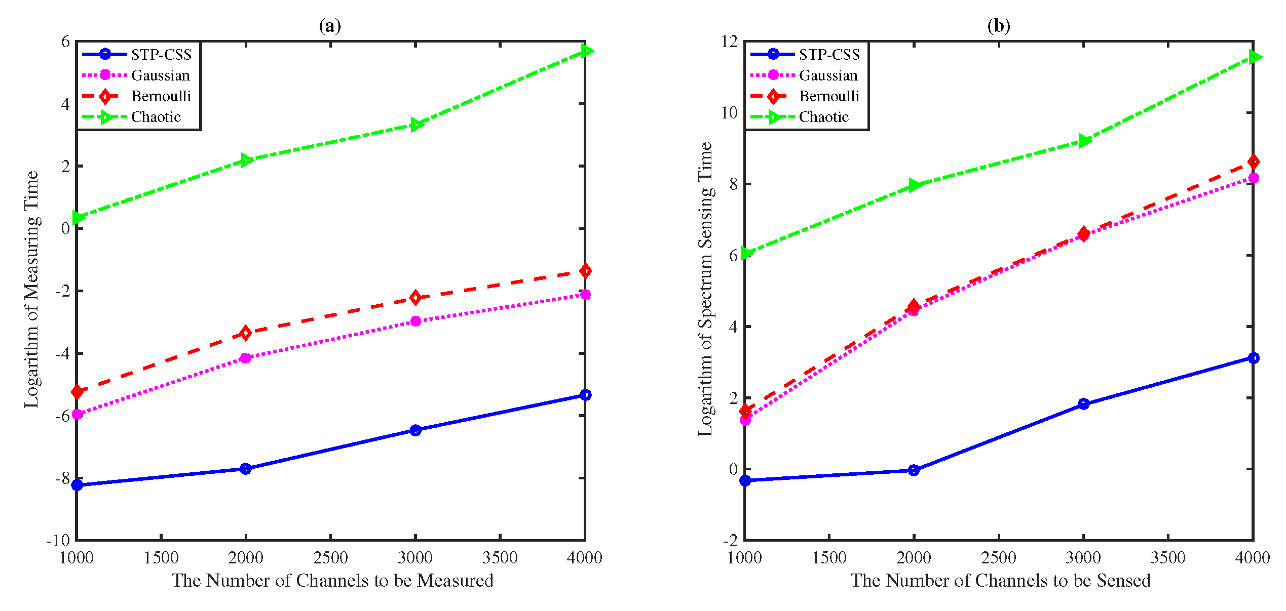
4.4. Running Time
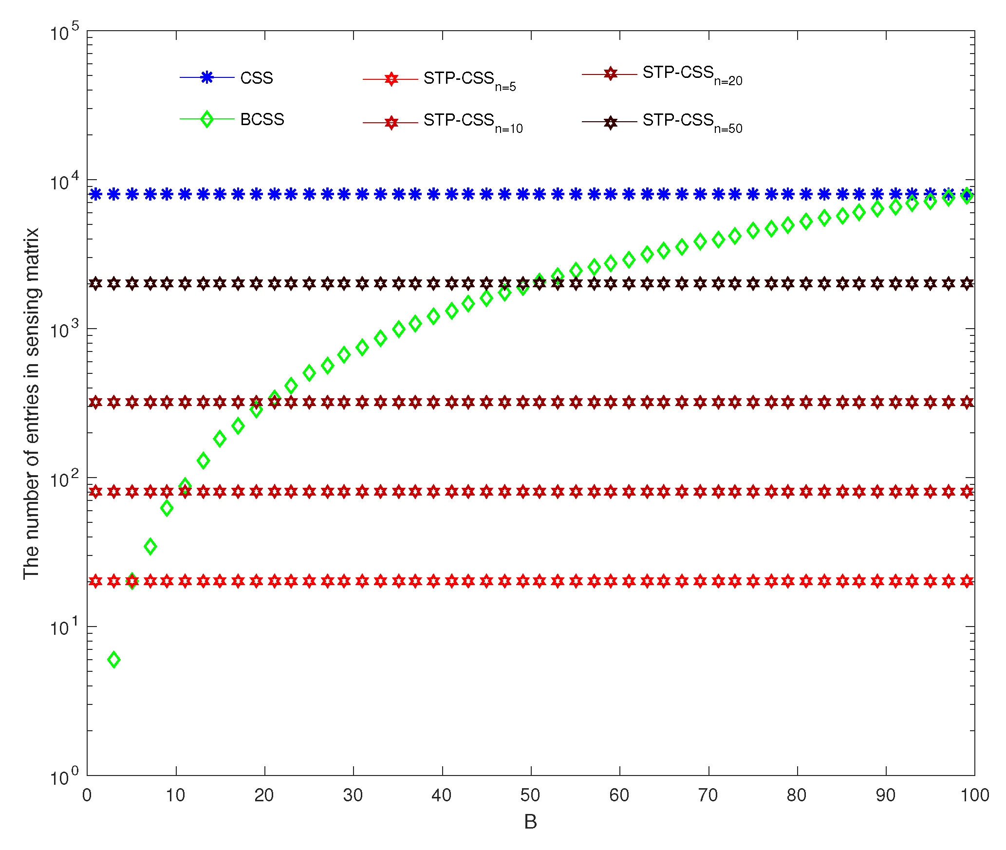
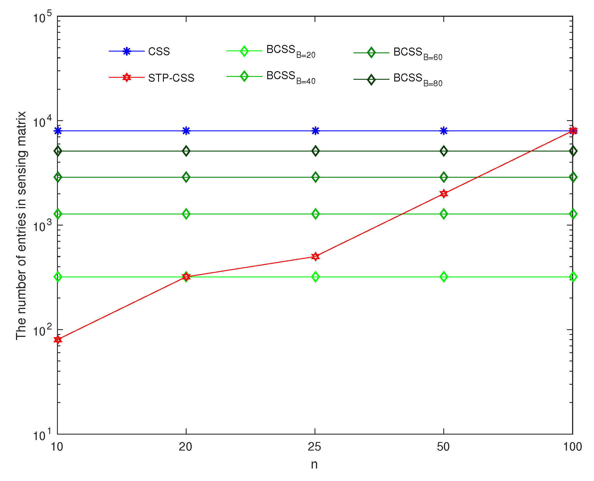
4.5. Storage Space
5. Conclusions
Author Contributions
Funding
Conflicts of Interest
Abbreviations
| CR | Cognitive radio |
| CRN | Cognitive radio network |
| CS | Compressed sensing |
| STP-CSS | Semi-tensor product compressed spectrum sensing |
| FCC | Federal Communications Commission |
| SU | Secondary user |
| PU | Primary user |
| DSA | Dynamic spectrum access |
| IoT | Cognitive radio network |
| 5G | The fifth generation wireless systems |
| NSS | Narrowband spectrum sensing |
| WSS | Wideband spectrum sensing |
| ADC | Analog-to-digital converter |
| CSS | Compressed spectrum sensing |
| AIC | Analog-to-information converter |
| MWC | Modulation wideband converter |
| RIP | Restricted isometry property |
| OMP | orthogonal matching pursuit |
| MP | Matching pursuit |
| ROMP | regular orthogonal matching pursuit |
| STP | Semi-tensor product |
| AWGN | Additive white Gaussian noise |
| DFT | Discrete Fourier transformation |
| BCS | Block-based compressed sensing |
References
- Federal Communications Commission. Spectrum Policy Task Force Report; Technical Report 02-135, ET Docket; Federal Communications Commission: Washington, DC, USA, 2002.
- Federal Communications Commission. Facilitating Opportunities for Flexible, Efficient, and Reliable Spectrum Use Employing Cognitive Radio Technologies; Technical Report 03-108; Federal Communications Commission: Washington, DC, USA, 2005.
- Hamdaoui, B.; Khalfi, B.; Guizani, M. Compressed wideband spectrum sensing: Concept, challenges and enablers. IEEE Commun. Mag. 2018, 56, 136–141. [Google Scholar] [CrossRef]
- Mitola, J.; Maguire, G.Q. Cognitive radio: Making software radios more personal. IEEE Pers. Commun. 1999, 6, 13–18. [Google Scholar] [CrossRef]
- Chiwewe, T.M.; Mbuya, C.F.; Hancke, G.P. Using cognitive radio for interference-resistant industrial wireless sensor networks: An overview. IEEE Trans. Ind. Informat. 2015, 11, 1466–1481. [Google Scholar] [CrossRef]
- Shakeel, A.; Hussain, R.; Iqbal, A.; Khan, I.L.; Hasan, Q.U.; Malik, S.A. Spectrum Handoff based on Imperfect Channel State Prediction Probabilities with Collision Reduction in Cognitive Radio Ad Hoc Networks. Sensors 2019, 19, 4741. [Google Scholar] [CrossRef] [PubMed]
- Arjoune, Y.; Kaabouch, N. A Comprehensive Survey on Spectrum Sensing in Cognitive Radio Networks: Recent Advances, New Challenges, and Future Research Directions. Sensors 2019, 19, 126. [Google Scholar] [CrossRef] [PubMed]
- Bera, S.; Misra, S.; Vasilakos, A.V. Software-defined networking for Internet of Things: A Survey. IEEE Internet Things J. 2017, 4, 1994–2008. [Google Scholar] [CrossRef]
- Khalfi, B.; Hamdaoui, B.; Guizani, M. Extracting and exploiting inherent sparsity for efficient IoT support in 5G: Challenges and potential solutions. IEEE Wirel. Commun. 2017, 24, 68–73. [Google Scholar] [CrossRef]
- Chen, X.; Liu, S.; Lu, J.; Fan, P.; Letaief, K.B. Smart channel sounder for 5G IoT: From wireless big data to active communication. IEEE Access 2016, 4, 8888–8899. [Google Scholar] [CrossRef]
- Condoluci, M.; Araniti, G.; Mahmoodi, T.; Dohler, M. Enabling the IoT machine age with 5G: Machine-type multicast services for innovative real-time applications. IEEE Access 2016, 4, 5555–5569. [Google Scholar] [CrossRef]
- Ejaz, W.; Ibnkahla, M. Multiband spectrum sensing and resource allocation for IoT in cognitive 5G networks. IEEE Internet Things J. 2018, 5, 150–163. [Google Scholar] [CrossRef]
- Yucek, T.; Arslan, H. A survey of spectrum sensing algorithms for cognitive radio applications. IEEE Commun. Surv. Tuts. 2009, 11, 116–130. [Google Scholar] [CrossRef]
- Axell, E.; Leus, G.; Larsson, E.G.; Poor, H.V. Spectrum sensing for cognitive radio: State-ofthe-art and recent advances. IEEE Signal Process. Mag. 2012, 29, 101–116. [Google Scholar] [CrossRef]
- Donoho, D.L. Compressed sensing. IEEE Trans. Inf. Theory 2006, 52, 1289–1306. [Google Scholar] [CrossRef]
- Cande, E.J. Compressive sampling. In Proceedings of the International Congress of Mathematicians, Madrid, Spain, 22–30 August 2006; pp. 1433–1452. [Google Scholar]
- Tian, Z.; Giannakis, G.B. Compressed sensing for wideband cognitive radios. In Proceedings of the IEEE International Conference on Acoustics, Speech and Signal Processing, Honolulu, HI, USA, 15–20 April 2007. [Google Scholar]
- Tian, Z.; Tafesse, Y.; Sadler, B.M. Cyclic feature detection with sub-Nyquist sampling for wideband spectrum sensing. IEEE J. Sel. Topics Signal Process. 2012, 6, 58–69. [Google Scholar] [CrossRef]
- Kirolos, S.; Laska, J.; Wakin, M.; Duarte, M.; Baron, D.; Ragheb, T.; Massoud, Y.; Baraniuk, R. Analog-to-information conversion via random demodulation. In Proceedings of the IEEE Dallas/CAS Workshop on Design, Applications, Integration and Software, Richardson, TX, USA, 29–30 October 2006; pp. 71–74. [Google Scholar]
- Mishali, M.; Eldar, Y.C. From theory to practice: Sub-Nyquist sampling of sparse wideband analog signals. IEEE J. Sel. Topics Signal Process. 2010, 4, 375–391. [Google Scholar] [CrossRef]
- Havary-Nassab, V.; Hassan, S.; Valaee, S. Compressive detection for wide-band spectrum sensing. In Proceedings of the IEEE International Conference on Acoustics, Speech and Signal Processing, Dallas, TX, USA, 14–19 March 2014; pp. 3094–3097. [Google Scholar]
- Lu, Q.; Yang, S.; Liu, F. Wideband Spectrum Sensing Based on Riemannian Distance for Cognitive Radio Networks. Sensors 2017, 17, 661. [Google Scholar] [CrossRef] [PubMed]
- Zhang, X.; Ma, Y.; Qi, H.; Gao, Y.; Xie, Z.; Xie, Z.; Zhang, M.; Wang, X.; Wei, G.; Li, Z. Distributed compressive sensing augmented wideband spectrum sharing for cognitive IoT. IEEE Internet Things J. 2018, 5, 3234–3245. [Google Scholar] [CrossRef]
- Arjoune, Y.; Kaabouch, N. Wideband Spectrum Sensing: A Bayesian Compressive Sensing Approach. Sensors 2018, 18, 1839. [Google Scholar] [CrossRef]
- Wang, B.; Liu, K.J.R. Advances in cognitive radio networks: A survey. IEEE J. Sel. Topics Signal Process. 2011, 5, 5–23. [Google Scholar] [CrossRef]
- Shankar, S.; Cordeiro, C.; Challapali, K. Spectrum agile radios: Utilization and sensing architectures. In Proceedings of the IEEE International Symposium on New Frontiers in Dynamic Spectrum Access Networks, Baltimore, MD, USA, 8–11 November 2005; pp. 160–169. [Google Scholar]
- Candes, E.J.; Tao, T. Near-optimal signal recovery from random projections: Universal encoding strategies. IEEE Trans. Inform. Theory 2006, 52, 5406–5425. [Google Scholar] [CrossRef]
- Candes, E.J.; Eldar, Y.C.; Needell, D.; Crandall, P. Compressed sensing with coherent and redundant dictionaries. Appl. Comput. Harmonic Anal. 2011, 31, 59–73. [Google Scholar] [CrossRef]
- Haupt, J.; Bajwa, W.U.; Raz, G.; Nowak, R. Toeplitz compressed sensing matrices with applications to sparse channel estimation. IEEE Trans. Inform. Theory 2010, 56, 5862–5875. [Google Scholar] [CrossRef]
- Mallat, S.G.; Zhang, Z. Matching pursuits with time-frequency dictionaries. IEEE Trans. Signal Process. 1993, 41, 3397–3415. [Google Scholar] [CrossRef]
- Tropp, J.A.; Gilbert, A.C. Signal recovery from random measurements via orthogonal matching pursuit. IEEE Trans. Inform. Theory 2007, 53, 4655–4666. [Google Scholar] [CrossRef]
- Donoho, D.L.; Tsaig, Y.; Drori, I.; Starck, J.-L. Sparse solution of underdetermined systems of linear equations by stagewise orthogonal matching pursuit. IEEE Trans. Inform. Theory 2012, 58, 1094–1121. [Google Scholar] [CrossRef]
- Cheng, D.Z.; Qi, H.; Xue, A. A survey on semi-tensor product of matrices. J. Syst. Sci. Complex 2012, 20, 304–322. [Google Scholar] [CrossRef]
- Peng, H.; Tian, Y.; Kurths, J.; Li, L.; Yang, Y.; Wang, D. Secure and energy-efficient data transmission system based on chaotic compressive sensing in body-to-body networks. IEEE Trans. Biomed. Circuits Syst. 2017, 11, 558–573. [Google Scholar] [CrossRef]
- Xie, D.; Peng, H.; Li, L.; Yang, Y. Semi-tensor compressed sensing. Digit. Signal Process. 2016, 58, 85–92. [Google Scholar] [CrossRef]
- Wang, A.; Lin, F.; Jin, Z.; Xu, W. A Configurable Energy-Efficient Compressed Sensing Architecture with Its Application on Body Sensor Networks. IEEE Trans. Ind. Inform. 2016, 12, 15–27. [Google Scholar] [CrossRef]
- Li, L.; Wen, G.; Wang, Z.; Yang, Y. Efficient and Secure Image Communication System Based on Compressed Sensing for IoT Monitoring Applications. IEEE Trans. Multimedia 2020, 22, 82–95. [Google Scholar] [CrossRef]
- Gan, L. Block compressed sensing of natural images. In Proceedings of the 15th International Conference on Digital Signal Processing, Cardiff, Wales, UK, 1–4 July 2007; pp. 403–406. [Google Scholar]


| Notation | Value | Description |
|---|---|---|
| 0.02 | Received power | |
| 1 | Channel width | |
| 0.1 | Time offset | |
| 1 | Variance of noise | |
| 118 | Judgment threshold |
| Compression Ratio | n = 100 | n = 200 | n = 1000 | n = 2000 |
|---|---|---|---|---|
| 1 | 4.896 | 9.696 | 48.096 | 96.096 |
| 3.936 | 7.776 | 38.496 | 76.896 | |
| 3.552 | 7.008 | 34.656 | 69.12 | |
| 2.016 | 3.936 | 19.296 | 38.496 | |
| 1056 | 2.016 | 9.696 | 19.296 |
© 2020 by the authors. Licensee MDPI, Basel, Switzerland. This article is an open access article distributed under the terms and conditions of the Creative Commons Attribution (CC BY) license (http://creativecommons.org/licenses/by/4.0/).
Share and Cite
Fang, Y.; Li, L.; Li, Y.; Peng, H.; Yang, Y. Low Energy Consumption Compressed Spectrum Sensing Based on Channel Energy Reconstruction in Cognitive Radio Network. Sensors 2020, 20, 1264. https://doi.org/10.3390/s20051264
Fang Y, Li L, Li Y, Peng H, Yang Y. Low Energy Consumption Compressed Spectrum Sensing Based on Channel Energy Reconstruction in Cognitive Radio Network. Sensors. 2020; 20(5):1264. https://doi.org/10.3390/s20051264
Chicago/Turabian StyleFang, Yuan, Lixiang Li, Yixiao Li, Haipeng Peng, and Yixian Yang. 2020. "Low Energy Consumption Compressed Spectrum Sensing Based on Channel Energy Reconstruction in Cognitive Radio Network" Sensors 20, no. 5: 1264. https://doi.org/10.3390/s20051264
APA StyleFang, Y., Li, L., Li, Y., Peng, H., & Yang, Y. (2020). Low Energy Consumption Compressed Spectrum Sensing Based on Channel Energy Reconstruction in Cognitive Radio Network. Sensors, 20(5), 1264. https://doi.org/10.3390/s20051264