Robust Visual Ship Tracking with an Ensemble Framework via Multi-View Learning and Wavelet Filter

 ,
,  ,
, 

Abstract
1. Introduction
2. Methodology
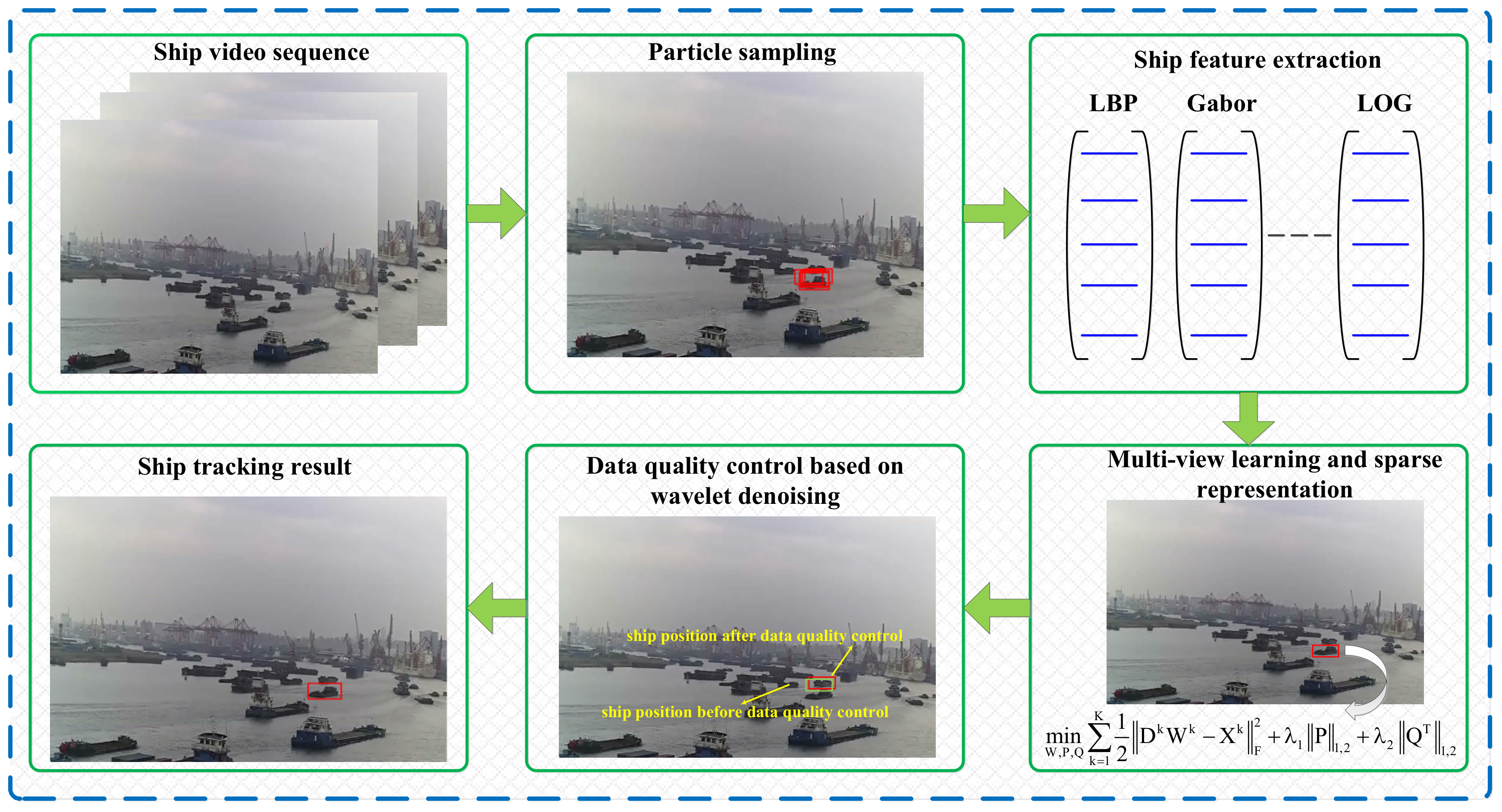
2.1. Framework Overview
2.2. Ship Training Candidates Sampling with PF Model
2.3. Ship Tracking with Multi-View Learning
2.3.1. Ship Feature Extraction
2.3.2. Establishing Ship Tracking Model with Multi-View Learning
2.3.3. Solving the Ship Tracking Model
2.4. Ship Position Denoising with WF Model
3. Experiments
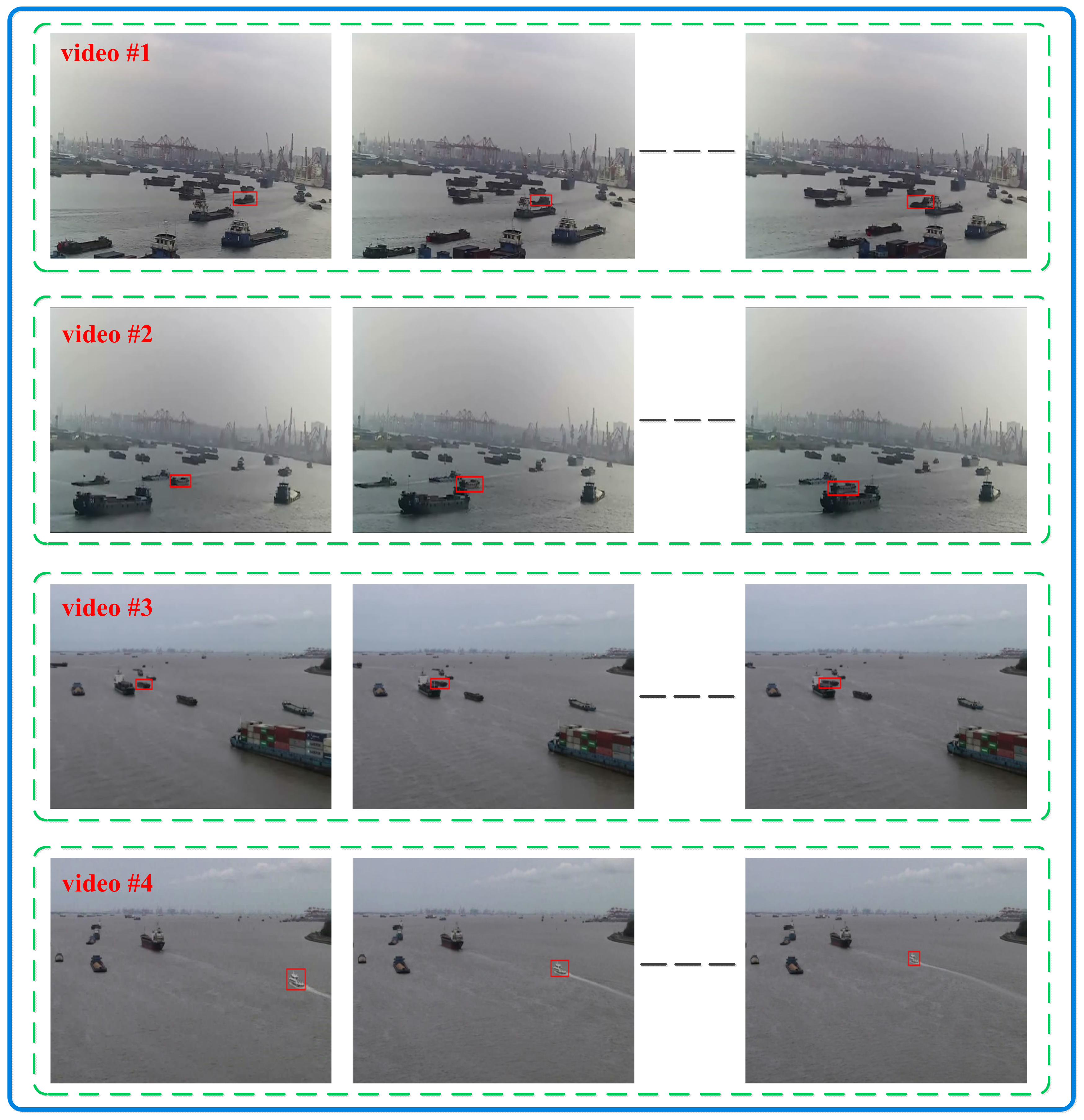
3.1. Data
3.2. Experimental Platform and Evaluation Criteria
3.3. Results
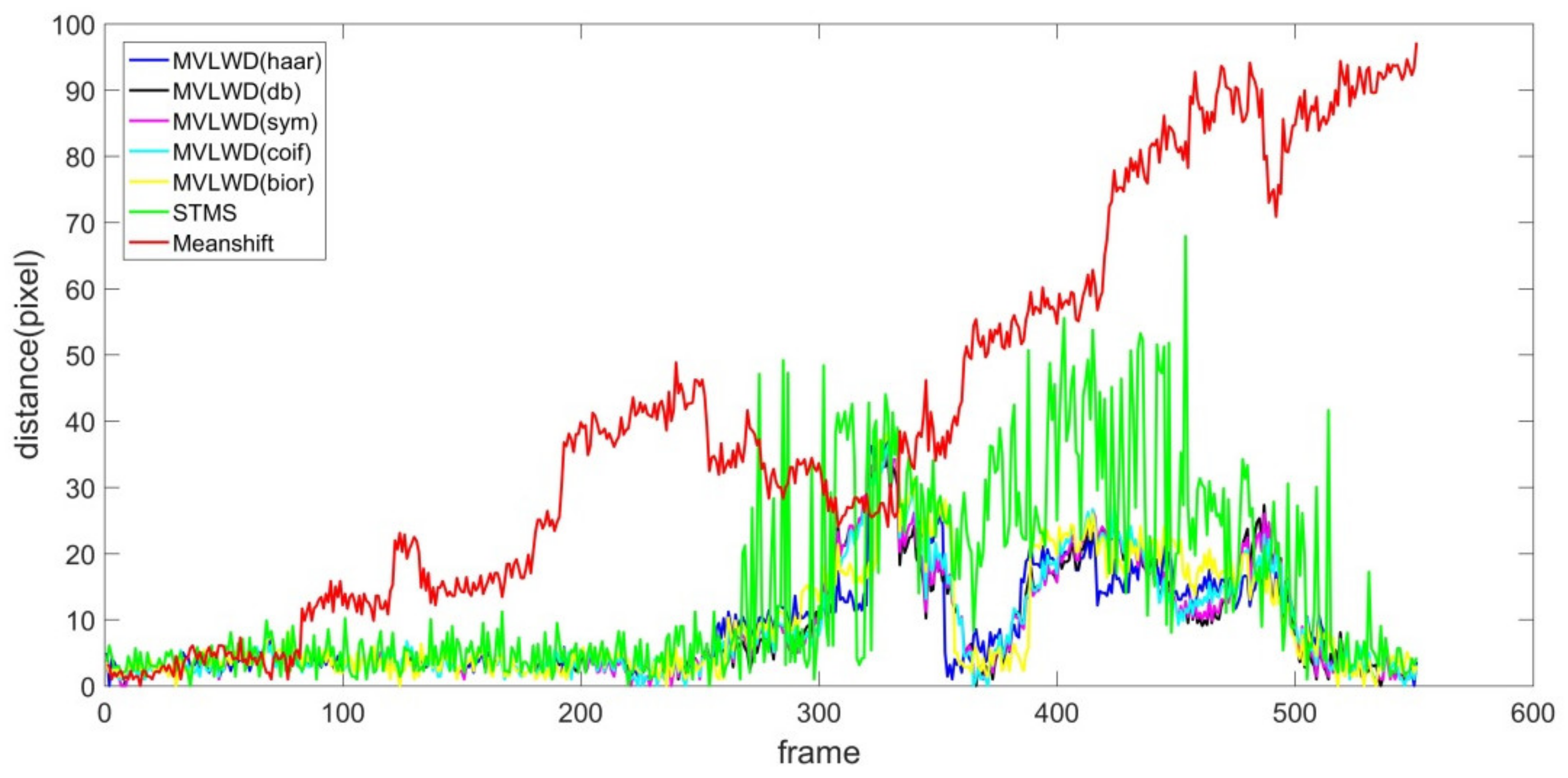
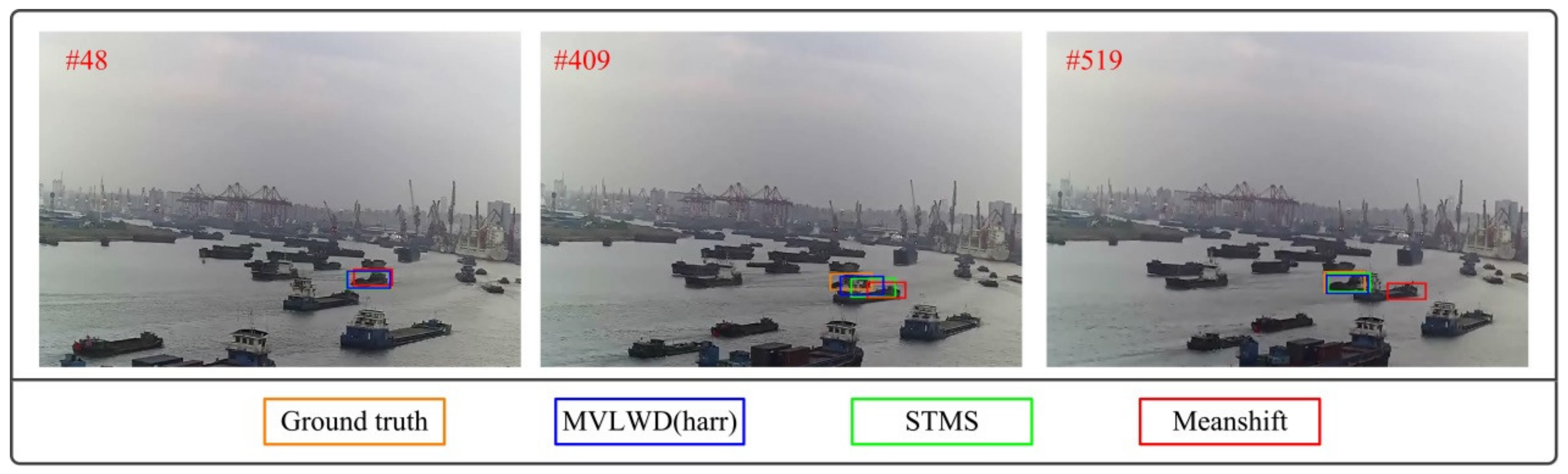
3.3.1. Ship Tracking Results for Video #1
3.3.2. Ship Tracking Results on Video #2
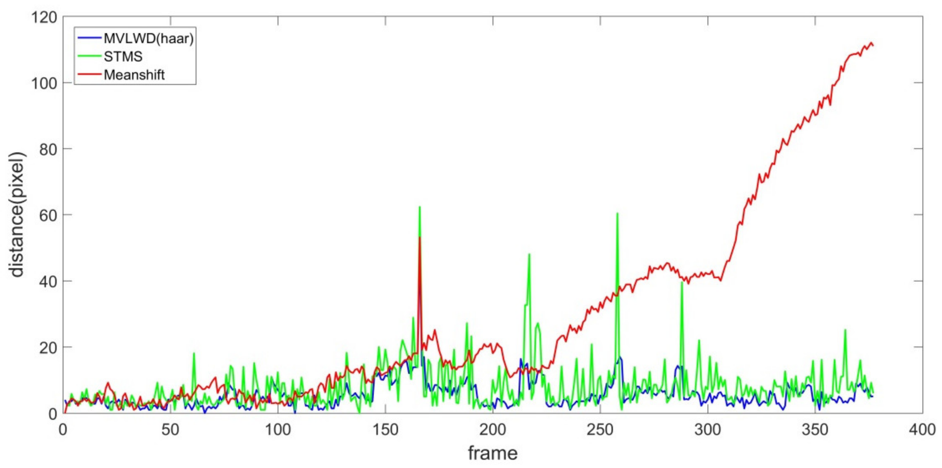
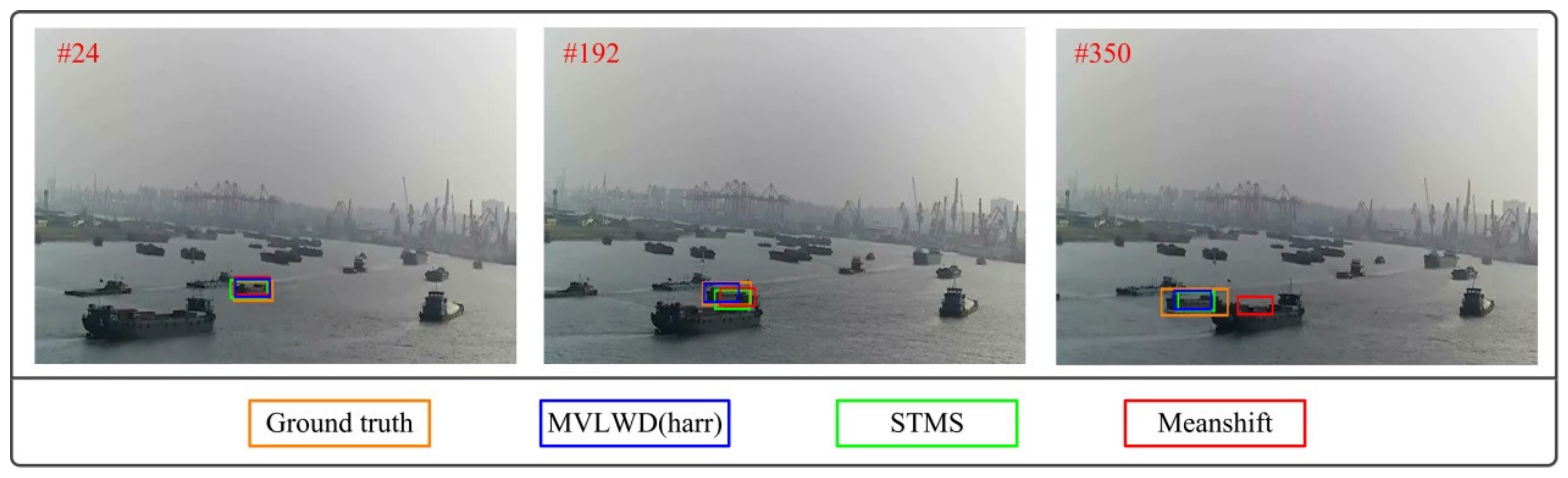
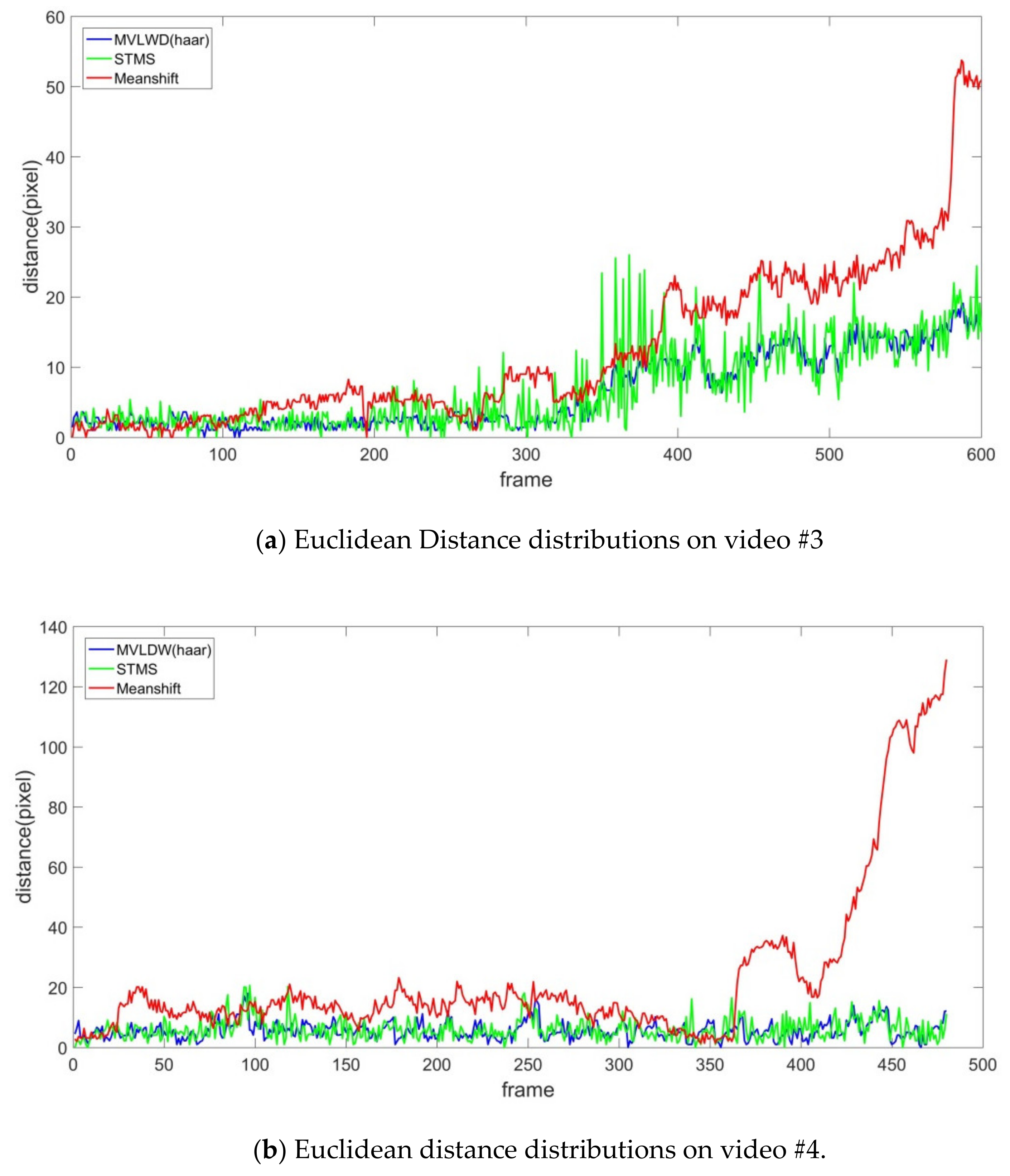
3.3.3. Ship Tracking Results for Videos #3 and #4
4. Conclusions
Author Contributions
Funding
Acknowledgments
Conflicts of Interest
References
- Bi, F.; Chen, J.; Zhuang, Y.; Bian, M.; Zhang, Q. A Decision Mixture Model-Based Method for Inshore Ship Detection Using High-Resolution Remote Sensing Images. Sensors 2017, 17, 1470. [Google Scholar] [CrossRef] [PubMed]
- Yao, L.; Liu, Y.; He, Y. A Novel Ship-Tracking Method for GF-4 Satellite Sequential Images. Sensors 2018, 18, 2007. [Google Scholar] [CrossRef] [PubMed]
- Ye, L.; Zong, Q. Tracking control of an underactuated ship by modified dynamic inversion. ISA Trans. 2018, 83, 100–106. [Google Scholar] [CrossRef] [PubMed]
- Tu, E.; Zhang, G.; Rachmawati, L.; Rajabally, E.; Huang, G.-B. Exploiting AIS Data for Intelligent Maritime Navigation: A Comprehensive Survey From Data to Methodology. IEEE Trans. Intell. Transp. Syst. 2018, 19, 1559–1582. [Google Scholar] [CrossRef]
- Pallotta, G.; Vespe, M.; Bryan, K. Vessel Pattern Knowledge Discovery from AIS Data: A Framework for Anomaly Detection and Route Prediction. Entropy 2013, 15, 2218–2245. [Google Scholar] [CrossRef]
- Xiu, S.; Wen, Y.; Yuan, H.; Xiao, C.; Zhan, W.; Zou, X.; Zhou, C.; Shah, S.C. A Multi-Feature and Multi-Level Matching Algorithm Using Aerial Image and AIS for Vessel Identification. Sensors 2019, 19, 1317. [Google Scholar] [CrossRef]
- Liu, W.; Zhen, Y.; Huang, J.; Zhao, Y. Inshore ship detection with high-resolution SAR data using salience map and kernel density. In Proceedings of the Eighth International Conference on Digital Image Processing (ICDIP 2016), Chengdu, China, 20–22 May 2016. [Google Scholar]
- Tian, S.; Wang, C.; Zhang, H. Ship detection method for single-polarization synthetic aperture radar imagery based on target enhancement and nonparametric clutter estimation. J. Appl. Remote Sens. 2015, 9, 096073. [Google Scholar] [CrossRef]
- Wang, Q.; Zhu, H.; Wu, W.; Zhao, H.; Yuan, N. Inshore ship detection using high-resolution synthetic aperture radar images based on maximally stable extremal region. J. Appl. Remote Sens. 2015, 9, 095094. [Google Scholar] [CrossRef]
- Chen, X.; Wang, S.; Shi, C.; Wu, H.; Zhao, J.; Fu, J. Robust Ship Tracking via Multi-view Learning and Sparse Representation. J. Navig. 2019, 72, 176–192. [Google Scholar] [CrossRef]
- Chong, J.; Wang, X.; Wei, X. Local region power spectrum-based unfocused ship detection method in synthetic aperture radar images. J. Appl. Remote Sens. 2018, 12. [Google Scholar] [CrossRef]
- Chaturvedi, S.K. Study of synthetic aperture radar and automatic identification system for ship target detection. J. Ocean Eng. Sci. 2019, 4, 173–182. [Google Scholar] [CrossRef]
- Chaturvedi, S.K.; Yang, C.-S.; Ouchi, K.; Shanmugam, P. Ship recognition by integration of SAR and AIS. J. Navig. 2012, 65, 323–337. [Google Scholar] [CrossRef]
- Lang, H.; Wu, S.; Xu, Y. Ship classification in SAR images improved by AIS knowledge transfer. IEEE Geosci. Remote Sens. Lett. 2018, 15, 439–443. [Google Scholar] [CrossRef]
- Leclerc, M.; Tharmarasa, R.; Florea, M.C.; Boury-Brisset, A.-C.; Kirubarajan, T.; Duclos-Hindié, N. Ship classification using deep learning techniques for maritime target tracking. In Proceedings of the 2018 21st International Conference on Information Fusion (FUSION), Cambridge, UK, 10 July 2018. [Google Scholar]
- Mahfouz, S.; Mourad-Chehade, F.; Honeine, P.; Farah, J.; Snoussi, H. Target Tracking Using Machine Learning and Kalman Filter in Wireless Sensor Networks. IEEE Sens. J. 2014, 14, 3715–3725. [Google Scholar] [CrossRef]
- Ristani, E.; Tomasi, C. Features for Multi-target Multi-camera Tracking and Re-identification. In Proceedings of the 2018 IEEE/CVF Conference on Computer Vision and Pattern Recognition, Salt Lake City, UT, USA, 18–22 June 2018. [Google Scholar]
- Prasad, D.K.; Rajan, D.; Rachmawati, L.; Rajabally, E.; Quek, C. Video Processing From Electro-Optical Sensors for Object Detection and Tracking in a Maritime Environment: A Survey. IEEE Trans. Intell. Transp. Syst. 2017, 18, 1993–2016. [Google Scholar] [CrossRef]
- Hu, H.; Guo, Q.; Zheng, J.; Wang, H.; Li, B. Single Image Defogging Based on Illumination Decomposition for Visual Maritime Surveillance. IEEE Trans. Image Process. 2019, 28, 2882–2897. [Google Scholar] [CrossRef]
- Guo, Q.; Feng, W.; Zhou, C.; Huang, R.; Wan, L.; Wang, S. Learning dynamic siamese network for visual object tracking. In Proceedings of the IEEE International Conference on Computer Vision, Venice, Italy, 22–29 October 2017. [Google Scholar]
- Zhu, Z.; Wang, Q.; Li, B.; Wu, W.; Yan, J.; Hu, W. Distractor-aware siamese networks for visual object tracking. In Proceedings of the European Conference on Computer Vision (ECCV), Munich, Germany, 8–14 September 2018. [Google Scholar]
- Park, J.; Kim, J.; Son, N.-S. Passive target tracking of marine traffic ships using onboard monocular camera for unmanned surface vessel. Electron. Lett. 2015. [Google Scholar] [CrossRef]
- Wawrzyniak, N.; Hyla, T.; Popik, A. Vessel Detection and Tracking Method Based on Video Surveillance. Sensors 2019, 19, 5230. [Google Scholar] [CrossRef]
- Kang, X.; Song, B.; Guo, J.; Du, X.; Guizani, M. A Self-Selective Correlation Ship Tracking Method for Smart Ocean Systems. Sensors 2019, 19, 821. [Google Scholar] [CrossRef]
- Zhang, Y.; Li, Q.-Z.; Zang, F.-N. Ship detection for visual maritime surveillance from non-stationary platforms. Ocean Eng. 2017, 141, 53–63. [Google Scholar] [CrossRef]
- Chen, X.; Yang, Y.; Wang, S.; Wu, H.; Tang, J.; Zhao, J.; Wang, Z. Ship Type Recognition via a Coarse-to-Fine Cascaded Convolution Neural Network. J. Navig. 2020. [Google Scholar] [CrossRef]
- Shao, Z.; Wang, L.; Wang, Z.; Du, W.; Wu, W. Saliency-Aware Convolution Neural Network for Ship Detection in Surveillance Video. IEEE Trans. Circuits Syst. Video Technol. 2019. [Google Scholar] [CrossRef]
- Zhang, W.; He, X.; Li, W.; Zhang, Z.; Luo, Y.; Su, L.; Wang, P. An integrated ship segmentation method based on discriminator and extractor. Image Vis. Comput. 2019, 103824. [Google Scholar] [CrossRef]
- Wu, Y.; Lim, J.; Yang, M.-H. Online object tracking: A benchmark. In Proceedings of the IEEE Conference on Computer Vision and Pattern Recognition, Portland, OR, USA, 25–27 June 2013. [Google Scholar]
- Hong, Z.; Chen, Z.; Wang, C.; Mei, X.; Prokhorov, D.; Tao, D. Multi-store tracker (muster): A cognitive psychology inspired approach to object tracking. In Proceedings of the IEEE Conference on Computer Vision and Pattern Recognition, Boston, MA, USA, 8–10 June 2015. [Google Scholar]
- Mei, X.; Ling, H. Robust visual tracking using ℓ 1 minimization. In Proceedings of the 2009 IEEE 12th International Conference on Computer Vision, Kyoto, Japan, 27 September–4 October 2009. [Google Scholar]
- Mei, X.; Hong, Z.; Prokhorov, D.; Tao, D. Robust Multitask Multiview Tracking in Videos. IEEE Trans. Neural Netw. Learn. Syst. 2015, 26, 2874–2890. [Google Scholar] [CrossRef] [PubMed]
- Mei, X.; Ling, H. Robust visual tracking and vehicle classification via sparse representation. IEEE Trans. Pattern Anal. Mach. Intell. 2011, 33, 2259–2272. [Google Scholar] [CrossRef] [PubMed]
- Hong, Z.; Mei, X.; Prokhorov, D.; Tao, D. Tracking via Robust Multi-task Multi-view Joint Sparse Representation. In Proceedings of the IEEE International Conference on Computer Vision, Sydney, Australia, 3–6 December 2013. [Google Scholar]
- Battiato, S.; Farinella, G.M.; Furnari, A.; Puglisi, G.; Snijders, A.; Spiekstra, J. An integrated system for vehicle tracking and classification. Expert Syst. Appl. 2015, 42, 7263–7275. [Google Scholar] [CrossRef]
- Wu, M.; Zhang, G.; Bi, N.; Xie, L.; Hu, Y.; Gao, S.; Shi, Z. Multiview vehicle tracking by graph matching model. In Proceedings of the Conference on Computer Vision and Pattern Recognition, Long Beach, CA, USA, 16–20 June 2019. [Google Scholar]
- Canny, J. A computational approach to edge detection. IEEE Trans. Pattern Anal. Mach. Intell. 1986, 8, 679–698. [Google Scholar] [CrossRef]
- Silvas, E.; Hereijgers, K.; Peng, H.; Hofman, T.; Steinbuch, M. Synthesis of Realistic Driving Cycles With High Accuracy and Computational Speed, Including Slope Information. IEEE Trans. Veh. Technol. 2016, 65, 4118–4128. [Google Scholar] [CrossRef]
- Xiao, L.; Xu, M.; Hu, Z. Real-Time Inland CCTV Ship Tracking. Math. Probl. Eng. 2018, 2018, 10. [Google Scholar] [CrossRef]
- Xiu, C.; Ba, F. Target tracking based on the improved Camshift method. In Proceedings of the 2016 Chinese Control and Decision Conference (CCDC), Yinchuan, China, 28–30 May 2016. [Google Scholar]
- Gong, P.; Ye, J.; Zhang, C. Robust multi-task feature learning. In Proceedings of the 18th ACM SIGKDD International Conference on Knowledge discovery and data mining, Beijing, China, 12–16 August 2012. [Google Scholar]
- Wang, S.; Ji, B.; Zhao, J.; Liu, W.; Xu, T. Predicting ship fuel consumption based on LASSO regression. Transp. Res. Part D Transp. Environ. 2018, 65, 817–824. [Google Scholar] [CrossRef]
- Zhou, Y.; Bai, X.; Liu, W.; Latecki, L.J. Similarity fusion for visual tracking. Int. J. Comput. Vis. 2016, 118, 337–363. [Google Scholar] [CrossRef]
- Zhang, Y.; Zhou, G.; Zhao, Q.; Cichocki, A.; Wang, X. Fast nonnegative tensor factorization based on accelerated proximal gradient and low-rank approximation. Neurocomputing 2016, 198, 148–154. [Google Scholar] [CrossRef]
- Verma, M.; Shukla, K.K. A new accelerated proximal gradient technique for regularized multitask learning framework. Pattern Recognit. Lett. 2017, 95, 98–103. [Google Scholar] [CrossRef]
- Liu, J.; Ji, S.; Ye, J. Multi-task feature learning via efficient l 2, 1-norm minimization. In Proceedings of the Twenty-Fifth Conference on Uncertainty in Artificial Intelligence, Montreal, Canada, 18–21 June 2009. [Google Scholar]
- Naimi, H.; Adamou-Mitiche, A.B.H.; Mitiche, L. Medical image denoising using dual tree complex thresholding wavelet transform and Wiener filter. J. King Saud Univ. Comput. Inf. Sci. 2015, 27, 40–45. [Google Scholar] [CrossRef]
- Čehovin, L.; Leonardis, A.; Kristan, M. Visual object tracking performance measures revisited. IEEE Trans. Image Process. 2016, 25, 1261–1274. [Google Scholar]
- Comaniciu, D.; Ramesh, V.; Meer, P. Real-time tracking of non-rigid objects using mean shift. In Proceedings of the IEEE Conference on Computer Vision and Pattern Recognition, Hilton Head Island, CA, USA, 15 June 2000. [Google Scholar]
- Tang, J.; Chen, X.; Hu, Z.; Zong, F.; Han, C.; Li, L. Traffic flow prediction based on combination of support vector machine and data denoising schemes. Phys. A Stat. Mech. Appl. 2019, 534, 120642. [Google Scholar] [CrossRef]


| MD (Pixels) | RMSE (Pixels) | MAE (Pixels) | |
|---|---|---|---|
| Meanshift | 41.01 | 29.41 | 24.70 |
| STMS | 14.03 | 14.16 | 11.93 |
| MVLWD (haar) | 8.54 | 7.73 | 6.24 |
| MVLWD (db) | 8.46 | 7.94 | 6.55 |
| MVLWD (sym) | 8.57 | 8.08 | 6.64 |
| MVLWD (coif) | 8.74 | 8.11 | 6.67 |
| MVLWD (bior) | 9.15 | 8.41 | 7.12 |
| MD (Pixels) | RMSE (Pixels) | MAE (Pixels) | |
|---|---|---|---|
| Meanshift | 29.15 | 30.21 | 24.15 |
| STMS | 7.87 | 7.29 | 4.78 |
| MVLWD (haar) | 5.44 | 4.16 | 2.80 |
| MD (Pixels) | RMSE (Pixels) | MAE (Pixels) | |
|---|---|---|---|
| Meanshift | 12.33 | 11.45 | 9.40 |
| STMS | 6.83 | 5.88 | 5.09 |
| MVLWD (haar) | 6.34 | 5.22 | 4.78 |
| MD (Pixels) | RMSE (Pixels) | MAE (Pixels) | |
|---|---|---|---|
| Meanshift | 23.28 | 26.92 | 17.17 |
| STMS | 5.99 | 3.60 | 2.79 |
| MVLWD (haar) | 5.57 | 2.93 | 2.28 |
© 2020 by the authors. Licensee MDPI, Basel, Switzerland. This article is an open access article distributed under the terms and conditions of the Creative Commons Attribution (CC BY) license (http://creativecommons.org/licenses/by/4.0/).
Share and Cite
Chen, X.; Chen, H.; Wu, H.; Huang, Y.; Yang, Y.; Zhang, W.; Xiong, P. Robust Visual Ship Tracking with an Ensemble Framework via Multi-View Learning and Wavelet Filter. Sensors 2020, 20, 932. https://doi.org/10.3390/s20030932
Chen X, Chen H, Wu H, Huang Y, Yang Y, Zhang W, Xiong P. Robust Visual Ship Tracking with an Ensemble Framework via Multi-View Learning and Wavelet Filter. Sensors. 2020; 20(3):932. https://doi.org/10.3390/s20030932
Chicago/Turabian StyleChen, Xinqiang, Huixing Chen, Huafeng Wu, Yanguo Huang, Yongsheng Yang, Wenhui Zhang, and Pengwen Xiong. 2020. "Robust Visual Ship Tracking with an Ensemble Framework via Multi-View Learning and Wavelet Filter" Sensors 20, no. 3: 932. https://doi.org/10.3390/s20030932
APA StyleChen, X., Chen, H., Wu, H., Huang, Y., Yang, Y., Zhang, W., & Xiong, P. (2020). Robust Visual Ship Tracking with an Ensemble Framework via Multi-View Learning and Wavelet Filter. Sensors, 20(3), 932. https://doi.org/10.3390/s20030932