3D Fast Object Detection Based on Discriminant Images and Dynamic Distance Threshold Clustering


Abstract
:1. Introduction
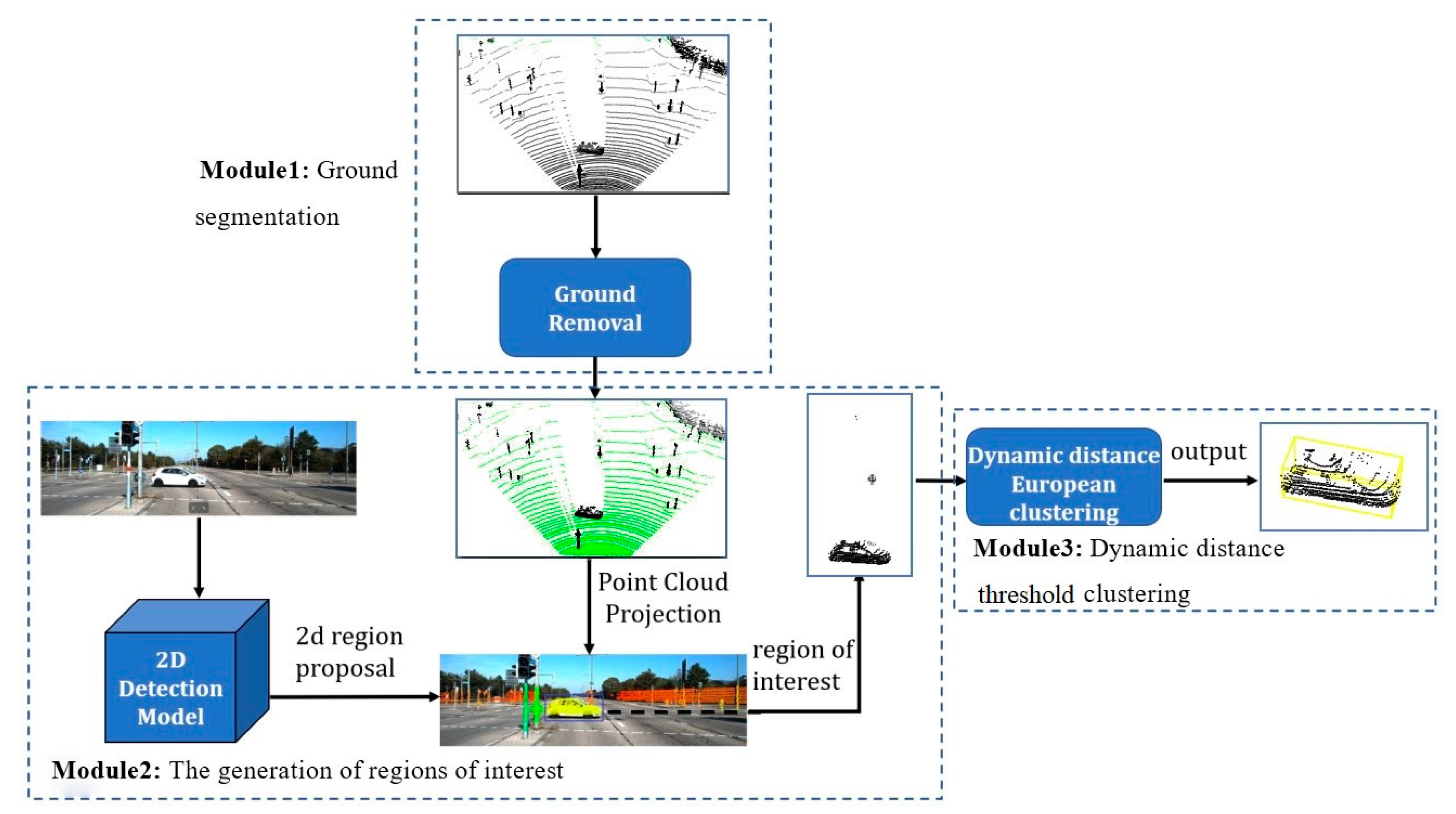
2. Three-Dimensional Fast Object Detection Algorithm
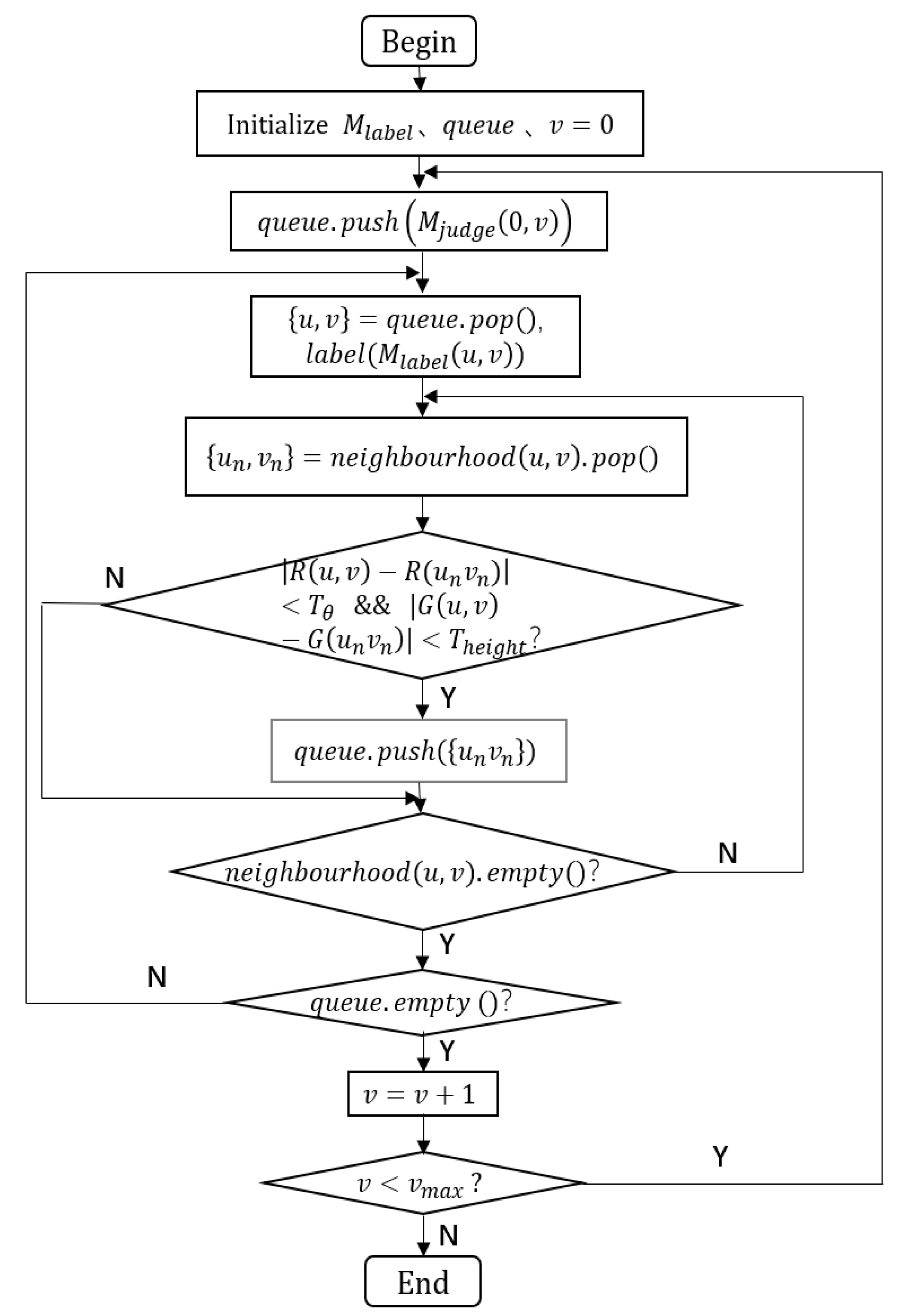
2.1. Ground Segmentation
- 1.
- First, create a label image,, equal to the size of and initialize it as a zero-value matrix. At the same time, create a queue for storing the current ground point.
- 2.
- Traverse from the first column of it and put the last element of the first column into queue.
- 3.
- Take out the first element of the queue and mark it as a ground point at the corresponding position of . Judge the four neighbor points of this point. If the R channel value difference (angle difference) between the neighbor point and this point meets the threshold condition, its G channel value difference (height difference) is also within the threshold range. This neighbor point is also marked as the ground point, so store it at the end of queue. Otherwise, judge the next neighbor point until all neighbor points have been judged.
- 4.
- Judge whether queue is null or not. If it is not null, then repeat Step 3. Otherwise, put the last element of the next column into the queue, and repeat Step 3, until all columns of have been traversed.
- 5.
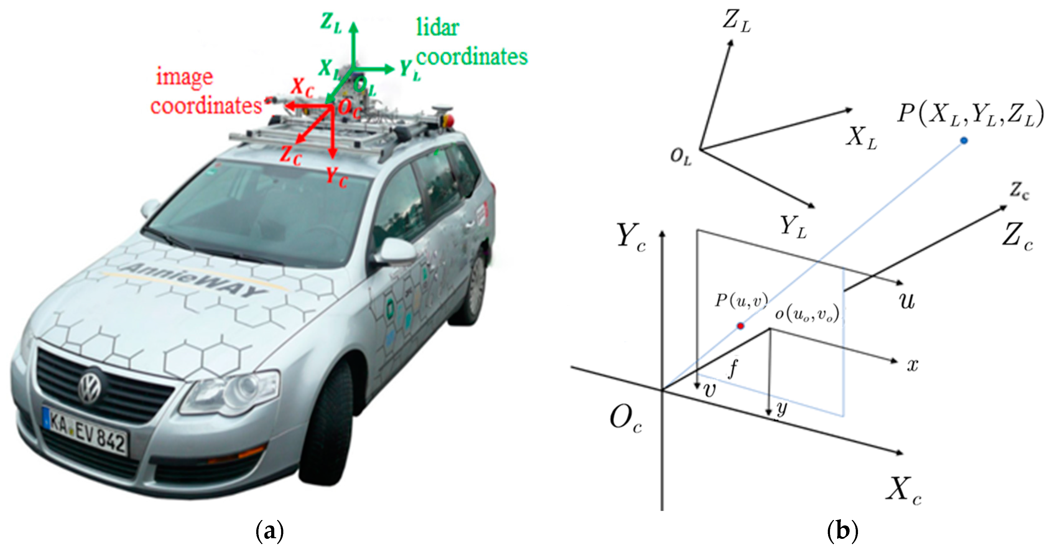
- According to the obtained label image, , the ground point is filtered out at the corresponding position on the lidar image, and then the lidar image without ground pixels is obtained, as shown in Figure 5. After obtaining the lidar image without ground pixels, point cloud can be projected into image, to obtain 3D point cloud without ground points.
2.2. Region of Interest
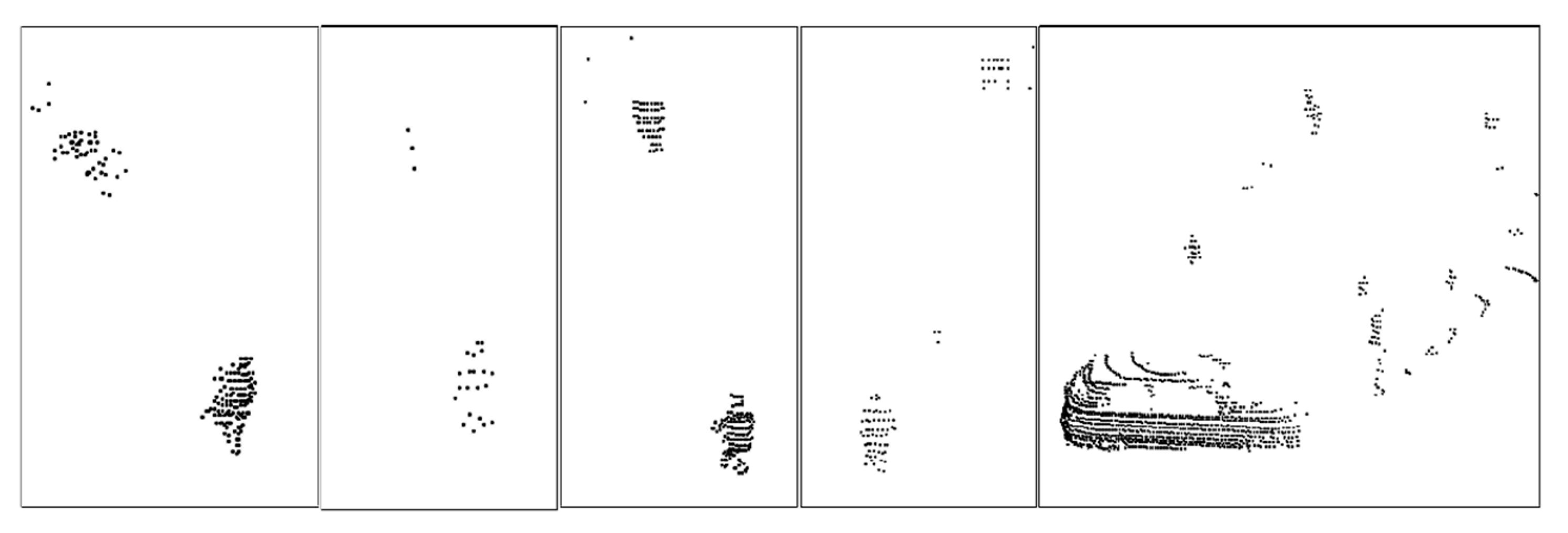
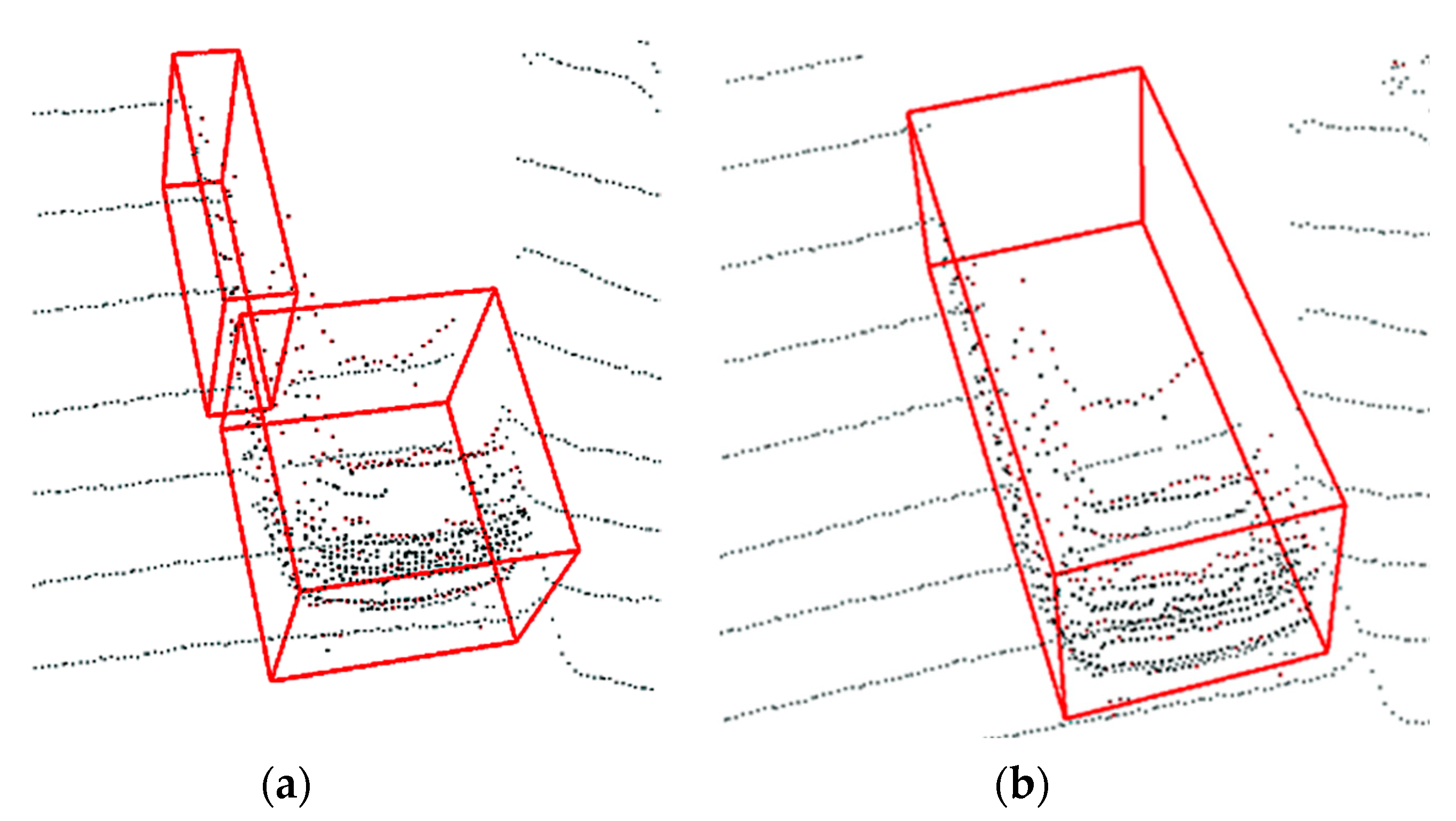
2.3. Dynamic Distance Threshold Clustering
3. Results and Discussion
3.1. Test Dataset and Evaluation Criteria
3.2. Comparative Analysis of Experimental Results
4. Experimental Analysis of each Module of the Algorithm
4.1. Ground Segmentation
4.2. Regions of Interest
4.3. Dynamic Distance Threshold Euclidean Clustering
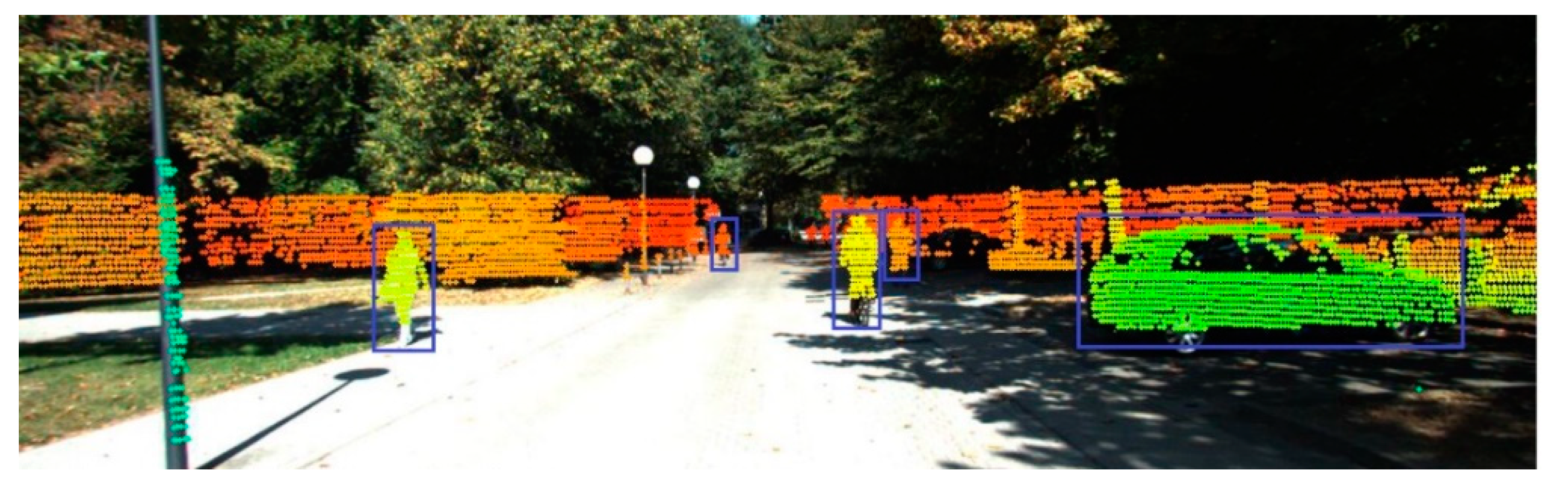
4.4. Visualized Results
5. Conclusions
Author Contributions
Funding
Conflicts of Interest
References
- Ren, S.; He, K.; Girshick, R.; Sun, J. Faster R-CNN: Towards Real-Time Object Detection with Region Proposal Networks. IEEE Trans. Pattern Anal. Mach. Intell. 2015, 39, 91–99. [Google Scholar] [CrossRef] [PubMed] [Green Version]
- Redmon, J.; Farhadi, A. Yolov3: An incremental improvement. In Proceedings of the Computer Vision and Pattern Recognition (CVPR), Salt Lake City, UT, USA, 18–22 June 2018; pp. 126–134. [Google Scholar]
- Sang, J.; Wu, Z.; Guo, P.; Hu, H.; Xiang, H.; Zhang, Q.; Cai, B. An Improved YOLOv2 for Vehicle Detection. Sensors 2018, 18, 4272. [Google Scholar] [CrossRef] [PubMed] [Green Version]
- Cao, J.; Song, C.; Song, S.; Peng, S.; Wang, D.; Shao, Y.; Xiao, F. Front Vehicle Detection Algorithm for Smart Car Based on Improved SSD Model. Sensors 2020, 20, 4646. [Google Scholar] [CrossRef] [PubMed]
- Geiger, A.; Lenz, P.; Urtasun, R. Are we ready for autonomous driving? The KITTI vision benchmark suite. In Proceedings of the Computer Vision and Pattern Recognition (CVPR), Providence, RI, USA, 16–21 June 2012; pp. 3354–3361. [Google Scholar]
- Chen, X.; Kundu, K.; Zhang, Z.; Ma, H.; Fidler, S.; Urtasun, R. Monocular 3d object detection for autonomous driving. In Proceedings of the IEEE Conference on Computer Vision and Pattern Recognition (CVPR), Las Vegas, NV, USA, 27–30 June 2016; pp. 2147–2156. [Google Scholar]
- Xiang, Y.; Choi, W.; Lin, Y.; Savarese, S. Data-driven 3d voxel patterns for object category recognition. In Proceedings of the IEEE Conference on Computer Vision and Pattern Recognition, Boston, MA, USA, 7–12 June 2015; pp. 1903–1911. [Google Scholar]
- Mousavian, A.; Anguelov, D.; Flynn, J.; Kosecka, J. 3D Bounding Box Estimation Using Deep Learning and Geometry. arXiv 2016, arXiv:1612.00496. [Google Scholar]
- Lindenberger, J. Laser Profilmessungen Zur Topographischen Gelndeaufnahme. Ph.D. Thesis, Verlag der Bay-erischen Akademic der Wissenschaften, Universitat Stnttgart, Stuttgart, Germany, 1993; p. 131. [Google Scholar]
- Stiene, S.; Lingemann, K.; Nuchter, A.; Hertzberg, J. Contour-based object detection in range images. In Proceedings of the Third International Symposium on 3D Data Processing, Visualization, and Transmission, Chapel Hill, NC, USA, 14–16 June 2006; pp. 168–175. [Google Scholar]
- Yao, W.; Hinz, S.; Stilla, U. 3D object-based classification for vehicle extraction from airborne LiDAR data by combining point shape information with spatial edge. In Proceedings of the 2010 IAPR Workshop on Pattern Recognition in Remote Sensing (PRRS), San Francisco, CA, USA, 13–18 June 2010; pp. 1–4. [Google Scholar]
- Ioannou, Y.; Taati, B.; Harrap, R.; Greenspan, M. Difference of normals as a multi-scale operator in unorganized point clouds. In Proceedings of the 2012 Second International Conference on 3D Imaging, Modeling, Processing, Visualization and Transmission (3DIMPVT), Zurich, Switzerland, 13–15 October 2012; pp. 501–508. [Google Scholar]
- Grilli, E.; Menna, F.; Remondino, F. A review of point clouds segmentation and classification algorithms. Int. Arch. Photogramm. Remote Sens. Spat. Inf. Sci. 2017, 42, 339–344. [Google Scholar] [CrossRef] [Green Version]
- Zhou, Y.; Tuzel, O. VoxelNet: End-to-End learning for point cloud based 3D object detection. In Proceedings of the 2018 IEEE Conference on Computer Vision and Pattern Recognition, Salt Lake City, UT, USA, 18–23 June 2018; pp. 4490–4499. [Google Scholar]
- Beltran, J.; Guindel, C.; Moreno, F.M.; Cruzado, D.; Garcia, F.; Escalera, A. BirdNet: A 3D object detection framework from LiDAR information. arXiv 2018, arXiv:1805.01195. [Google Scholar]
- Zeng, Y.; Hu, Y.; Liu, S.; Ye, J.; Han, Y.; Li, X.; Sun, N. RT3D: Real-Time 3-D Vehicle Detection in LiDAR Point Cloud for Autonomous Driving. IEEE Robot. Autom. Lett. 2018, 3, 3434–3440. [Google Scholar] [CrossRef]
- Mandikal, P.; Navaneet, K.L.; Agarwal, M.; Babu, R.V. 3D-LMNet: Latent Embedding Matching for Accurate and Diverse 3D Point Cloud Reconstruction from a Single Image. arXiv 2018, arXiv:1807.07796. [Google Scholar]
- Li, B.; Zhang, T.; Xia, T. Vehicle detection from 3D lidar using fully convolutional network. In Proceedings of the 2016 Robotics: Science and Systems Conference, Ann Arbor, MI, USA, 18–22 June 2016. [Google Scholar]
- Qi, C.R.; Su, H.; Mo, K.; Guibas, L.J. PointNet: Deep Learning on Point Sets for 3D Classification and Segmentation. arXiv 2016, arXiv:1612.00593. [Google Scholar]
- Qi, C.R.; Yi, L.; Su, H.; Guibas, L.J. PointNet++: Deep Hierarchical Feature Learning on Point Sets in a Metric Space. arXiv 2017, arXiv:1706.02413. [Google Scholar]
- Urmson, C.; Anhalt, J.; Bagnell, D.; Baker, C.; Bittner, R.; Clark, M.N.; Dolan, J.; Duggins, D.; Galatali, T.; Geyer, C.; et al. Chris Geyer Autonomous Driving in Urban Environments: Boss and the Urban Challenge. J. Field Robot. 2008, 25, 425–466. [Google Scholar] [CrossRef] [Green Version]
- Osep, A.; Hermans, A.; Engelmann, F.; Klostermann, D.; Mathias, M.; Leibe, B. Multi-Scale Object Candidates for Generic Object Tracking in Street Scenes. In Proceedings of the 2016 IEEE International Conference on Robotics and Automation (ICRA), Stockholm, Sweden, 16–21 May 2016. [Google Scholar]
- Bogoslavskyi, I.; Stachniss, C. Fast range image-based segmentation of sparse 3D laser scans for online operation. In Proceedings of the 2016 IEEE/RSJ International Conference on Intelligent Robots and Systems (IROS), Daejeon, Korea, 9–14 October 2016. [Google Scholar]
- He, K.; Gkioxari, G.; Dollár, P.; Girshick, R. Mask R-CNN. In Proceedings of the IEEE International Conference on Computer Vision, Venice, Italy, 22–29 October 2017; pp. 2017–2961. [Google Scholar]
- Li, S.; Wang, J.; Liang, Z.; Su, L. Tree point clouds registration using an improved ICP algorithm based on kd-tree. In Proceedings of the IGARSS 2016—2016 IEEE International Geoscience and Remote Sensing Symposium, Beijing, China, 10–15 July 2016. [Google Scholar]
- Qi, C.R.; Liu, W.; Wu, C.; Su, H.; Guibas, L.J. Frustum PointNets for 3D Object Detection from RGB-D Data. In Proceedings of the IEEE International Conference on Computer Vision and Pattern Recognition, Salt Lake City, UT, USA, 18–22 June 2018. [Google Scholar]


| Algorithms | AP loc (%) | |||||
|---|---|---|---|---|---|---|
| IoU = 0.5 | IoU = 0.7 | |||||
| Easy | Moderate | Hard | Easy | Moderate | Hard | |
| Mono3D | 30.50 | 22.39 | 19.16 | 5.22 | 5.19 | 4.13 |
| Deep3DBox | 29.96 | 24.91 | 19.46 | 9.01 | 7.94 | 6.57 |
| 3DOP | 55.04 | 41.25 | 34.55 | 12.63 | 9.49 | 7.59 |
| BirdNet | N/A | N/A | N/A | 35.52 | 30.81 | 30.00 |
| VeloFCN | 79.68 | 63.82 | 62.80 | 40.14 | 32.08 | 30.47 |
| F-PointNet | 88.70 | 84.00 | 75.33 | 50.22 | 58.09 | 47.20 |
| Our method | 83.23 | 71.74 | 70.28 | 49.45 | 43.65 | 40.39 |
| Algorithms | AP 3D (%) | |||||
|---|---|---|---|---|---|---|
| IoU = 0.5 | IoU = 0.7 | |||||
| Easy | Moderate | Hard | Easy | Moderate | Hard | |
| Mono3D | 25.19 | 18.20 | 15.52 | 2.53 | 2.31 | 2.31 |
| Deep3DBox | 24.76 | 21.95 | 16.87 | 5.40 | 5.66 | 3.97 |
| 3DOP | 46.04 | 34.63 | 30.09 | 6.55 | 5.07 | 4.10 |
| BirdNet | N/A | N/A | N/A | 14.75 | 13.44 | 12.04 |
| VeloFCN | 67.92 | 57.57 | 52.56 | 15.20 | 13.66 | 15.98 |
| F-PointNet | 81.20 | 70.39 | 62.19 | 51.21 | 44.89 | 40.23 |
| Our method | 74.68 | 63.81 | 60.12 | 32.79 | 29.64 | 21.82 |
| Algorithms | Mono3D | Deep3DBox | 3DOP | BirdNet | VeloFCN | F-PointNet | Our method |
| Time (ms) | 206 | 213 | 378 | 110 | 1000 | 170 | 74 |
| Algorithms | Runtime | Frequency |
|---|---|---|
| Grid map-based | 3.7 ms 0.2 ms | 270 Hz |
| Ground plane fitting-based | 24.6 ms 1.2 ms | 41 Hz |
| Our method | 5.5 ms 0.3 ms | 182 Hz |
| Method | Average Runtime |
|---|---|
| downsampling | 628 ms |
| region of interest | 74 ms |
| Distance | Number of Actual Objects | Traditional Euclidean Clustering Algorithm | Our Method | ||
|---|---|---|---|---|---|
| Number of Objects Detected Accurately | AP loc | Number of Objects Detected Accurately | AP loc | ||
| 0~10 m | 3128 | 2911 | 93.06 | 3014 | 96.35 |
| 10~20 m | 2952 | 2549 | 86.35 | 2639 | 89.39 |
| 20~30 m | 2577 | 2041 | 79.20 | 2285 | 88.67 |
| 30~40 m | 2705 | 1780 | 65.80 | 2341 | 86.55 |
| 40~50 m | 2384 | 791 | 33.18 | 1719 | 72.12 |
| 50~60 m | 2048 | 440 | 15.48 | 1312 | 64.05 |
Publisher’s Note: MDPI stays neutral with regard to jurisdictional claims in published maps and institutional affiliations. |
© 2020 by the authors. Licensee MDPI, Basel, Switzerland. This article is an open access article distributed under the terms and conditions of the Creative Commons Attribution (CC BY) license (http://creativecommons.org/licenses/by/4.0/).
Share and Cite
Chen, B.; Chen, H.; Yuan, D.; Yu, L. 3D Fast Object Detection Based on Discriminant Images and Dynamic Distance Threshold Clustering. Sensors 2020, 20, 7221. https://doi.org/10.3390/s20247221
Chen B, Chen H, Yuan D, Yu L. 3D Fast Object Detection Based on Discriminant Images and Dynamic Distance Threshold Clustering. Sensors. 2020; 20(24):7221. https://doi.org/10.3390/s20247221
Chicago/Turabian StyleChen, Baifan, Hong Chen, Dian Yuan, and Lingli Yu. 2020. "3D Fast Object Detection Based on Discriminant Images and Dynamic Distance Threshold Clustering" Sensors 20, no. 24: 7221. https://doi.org/10.3390/s20247221
APA StyleChen, B., Chen, H., Yuan, D., & Yu, L. (2020). 3D Fast Object Detection Based on Discriminant Images and Dynamic Distance Threshold Clustering. Sensors, 20(24), 7221. https://doi.org/10.3390/s20247221