BwimNet: A Novel Method for Identifying Moving Vehicles Utilizing a Modified Encoder-Decoder Architecture


Abstract
1. Introduction
2. Proposed BwimNet Method
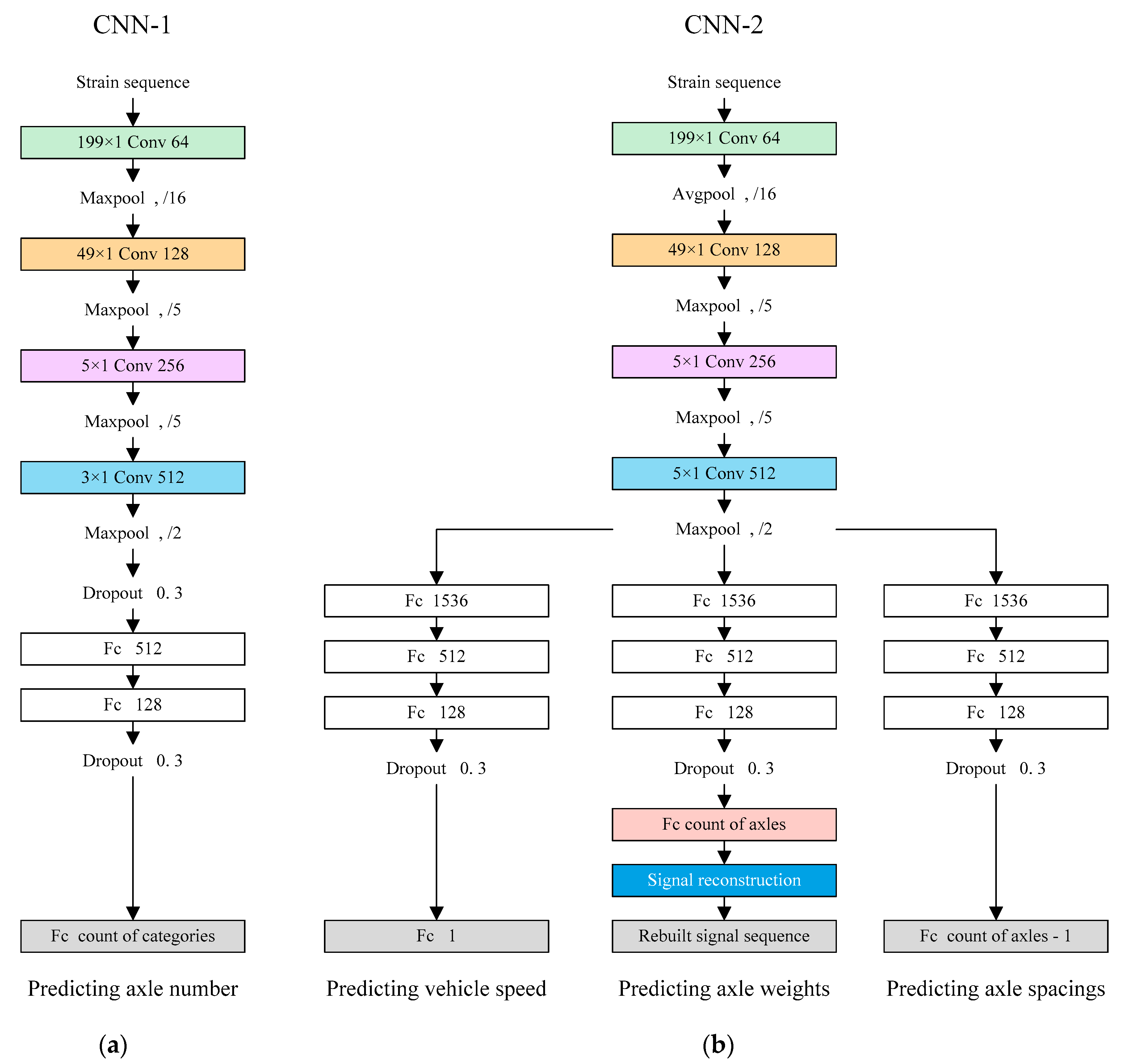
2.1. Axle Count Predicting
2.2. Velocity and Wheelbase Predicting
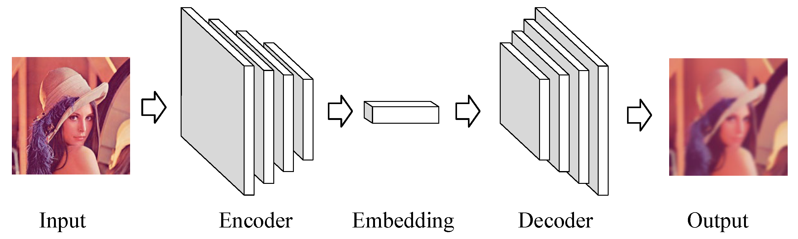
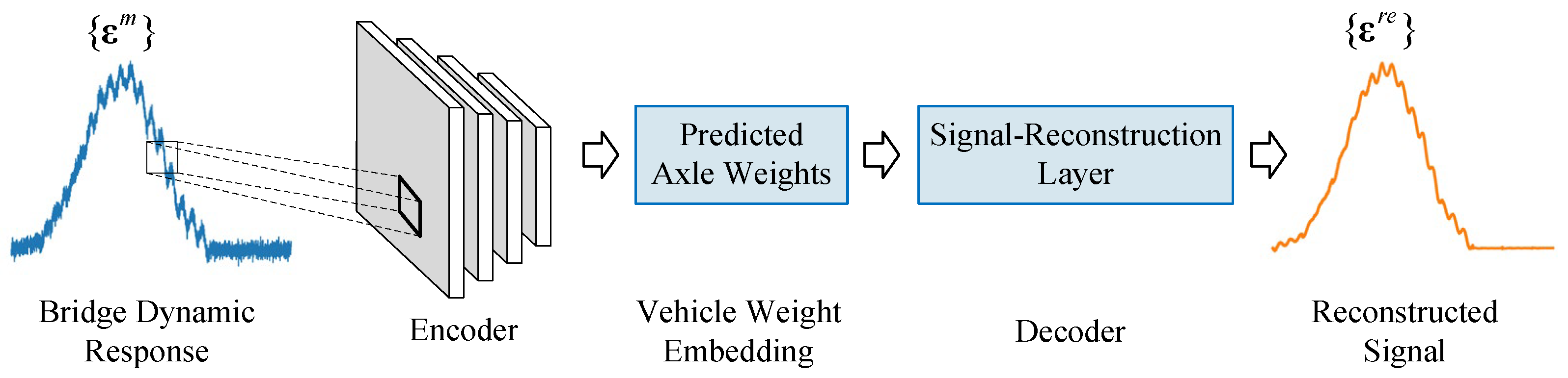
2.3. Vehicle Weight Predicting
3. Numerical Simulation
3.1. Vehicle-Bridge Coupling Vibration Model
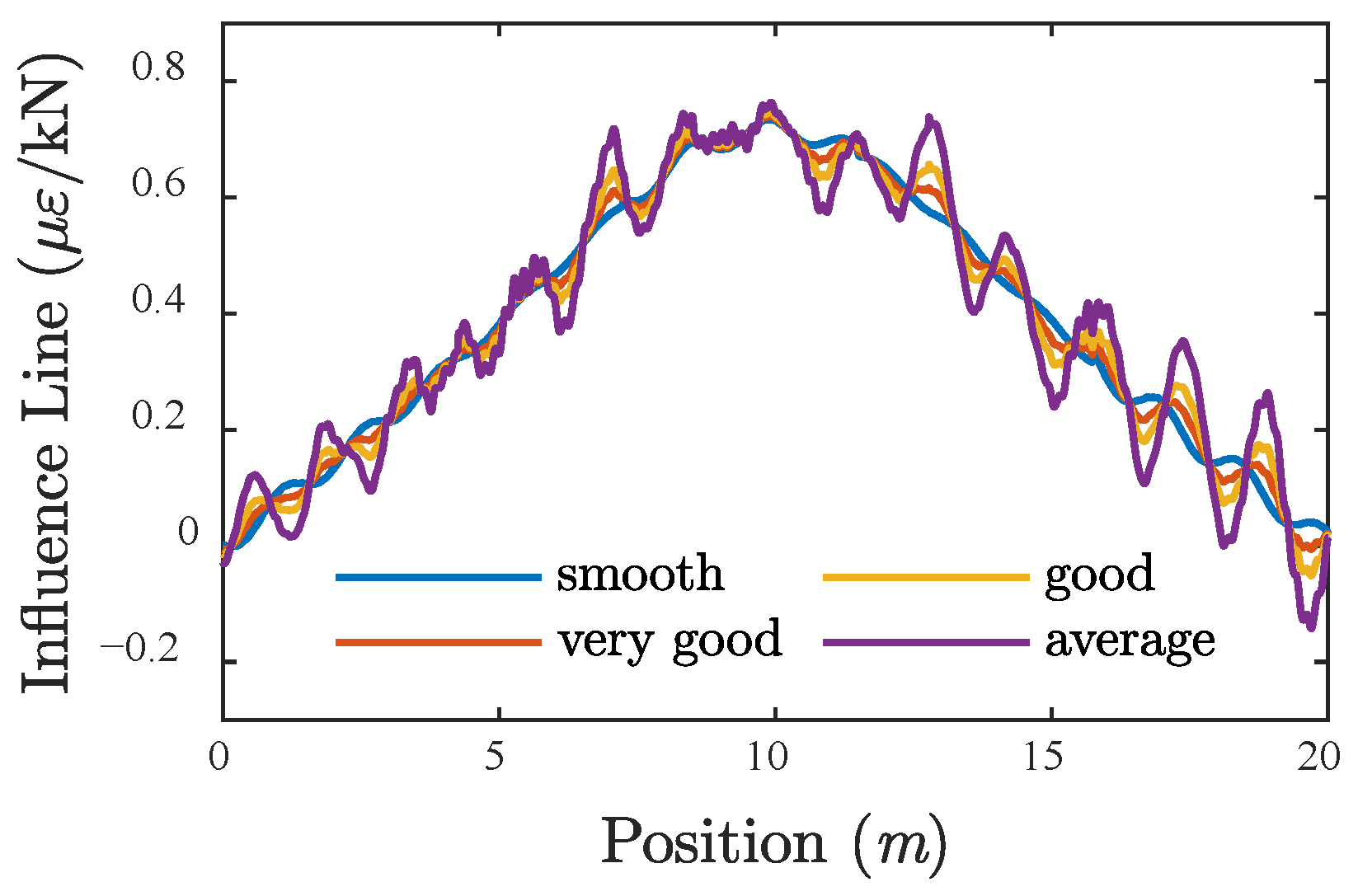
3.1.1. Road Surface Condition
3.1.2. Road Surface Condition
3.2. Simulation Setup
3.2.1. Vehicle Model
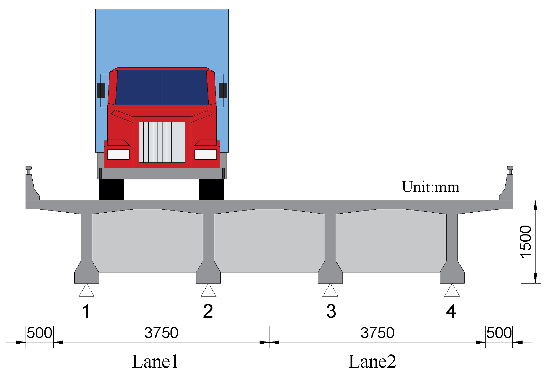
3.2.2. Bridge and Truck Models
3.2.3. Training and Evaluation Datasets
4. Results
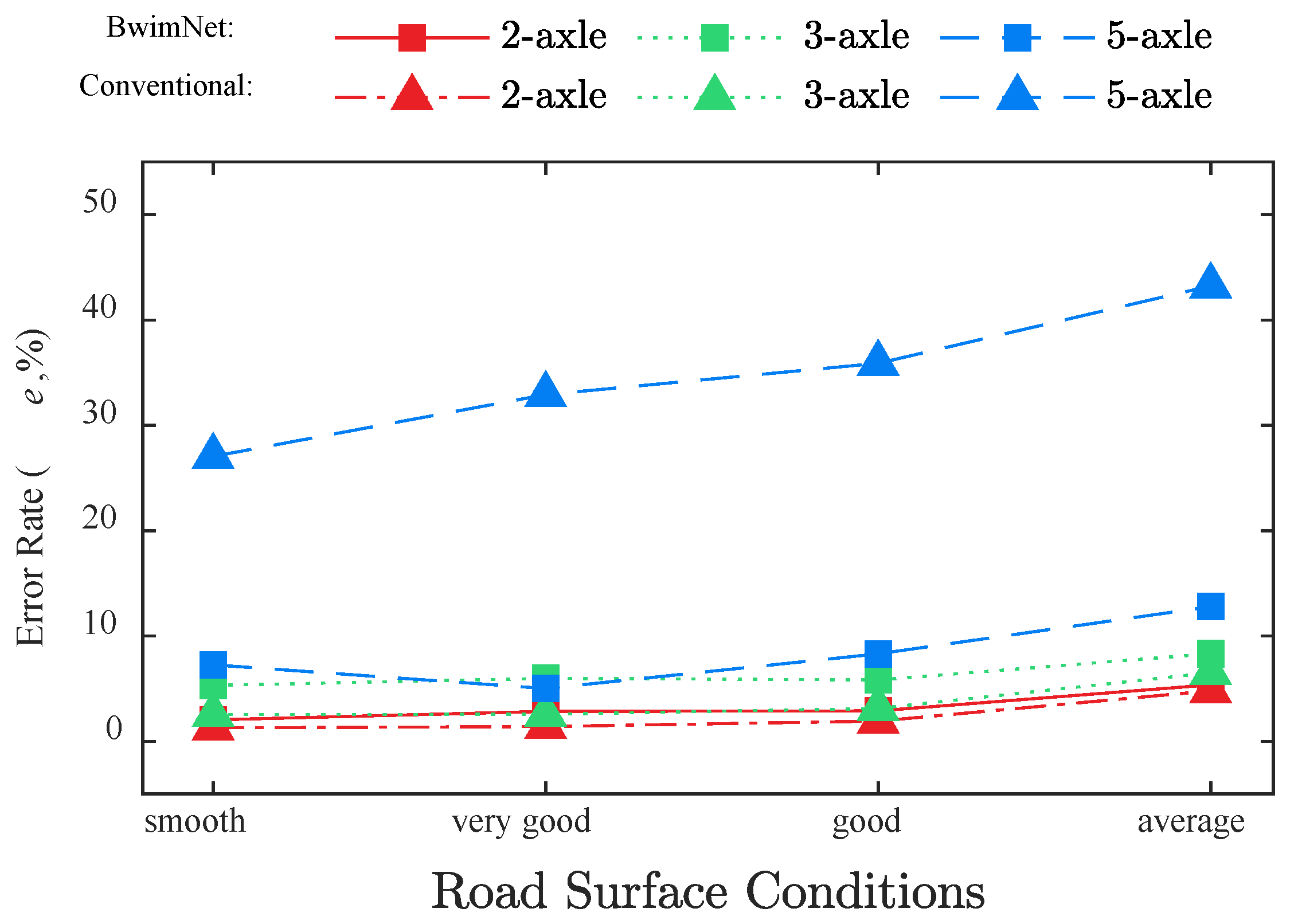
4.1. Comparison with Conventional BWIM Algorithm
4.2. Effect of Road Surface Condition
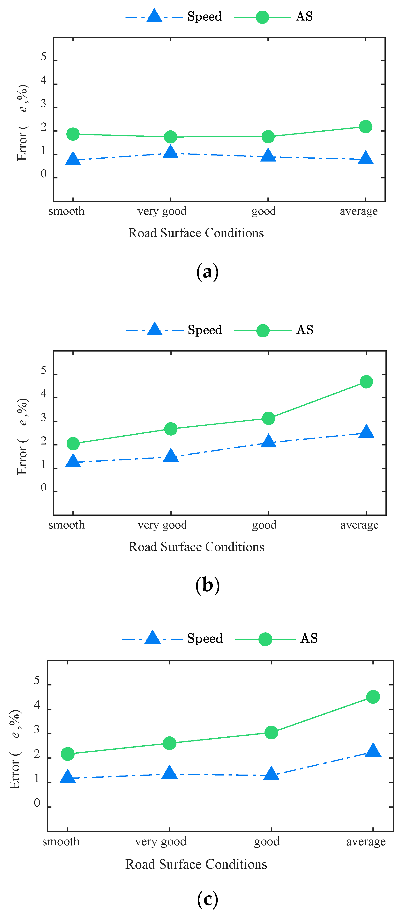
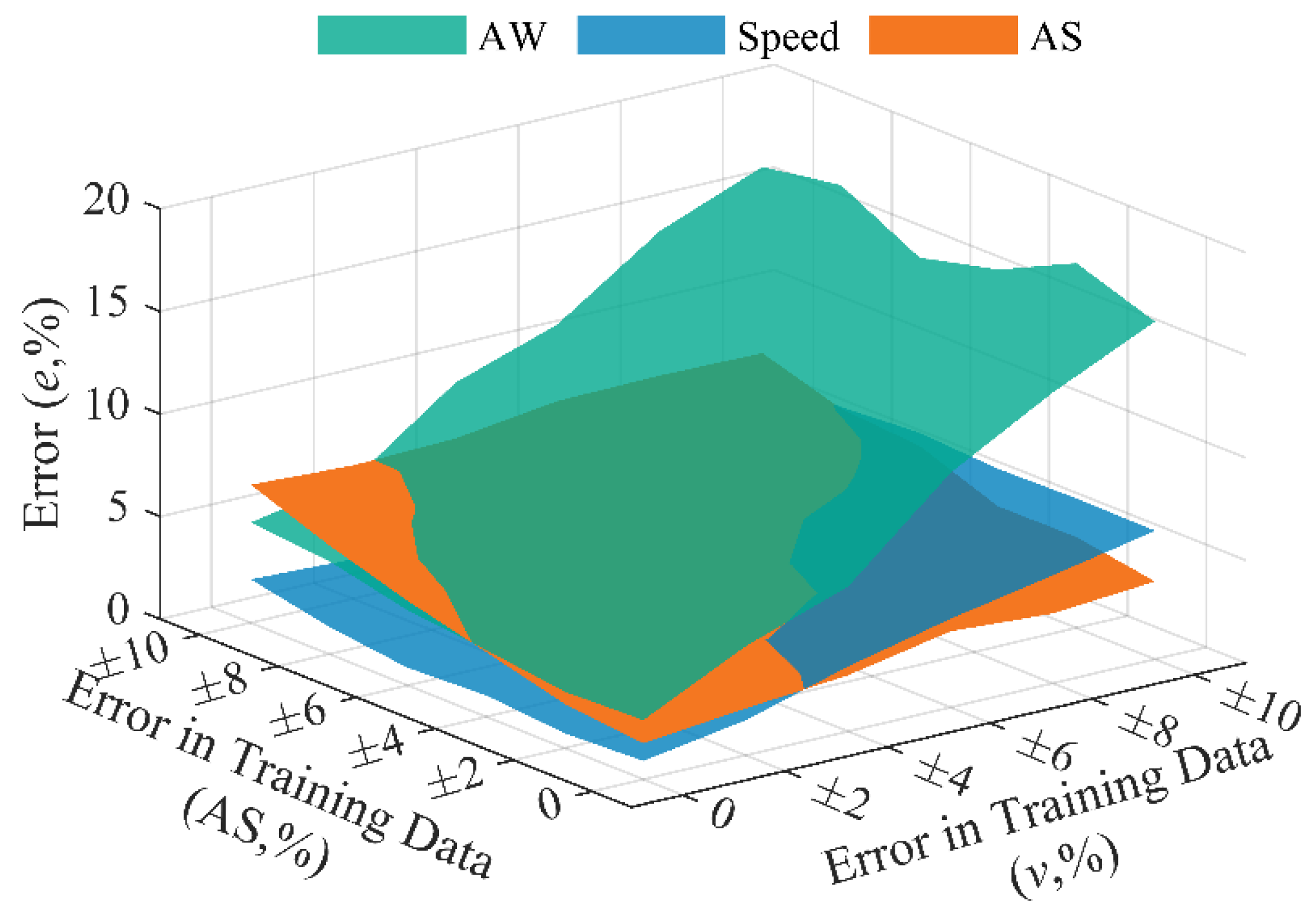
4.3. Effect of Error in Training Set of Speed and Wheelbase
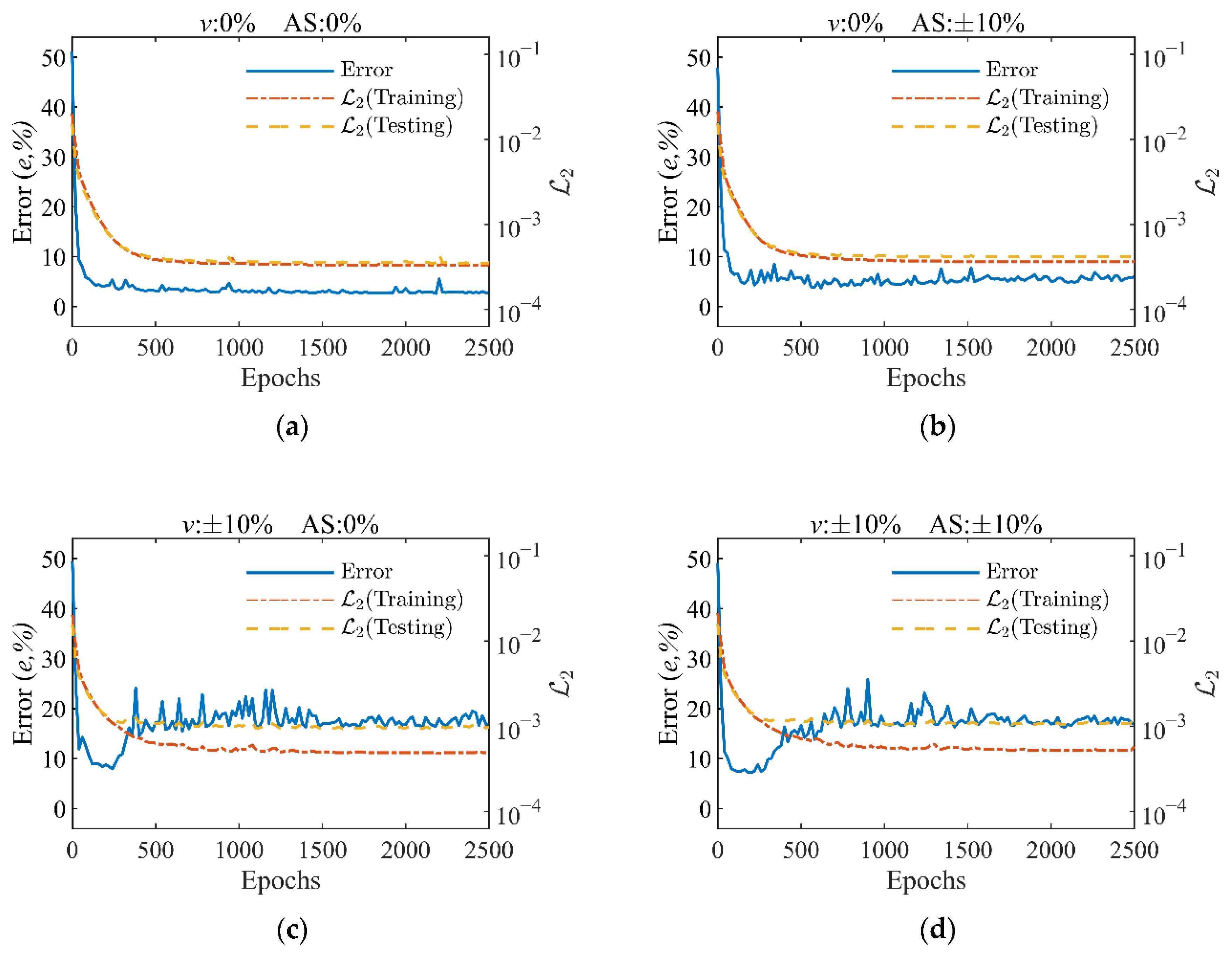
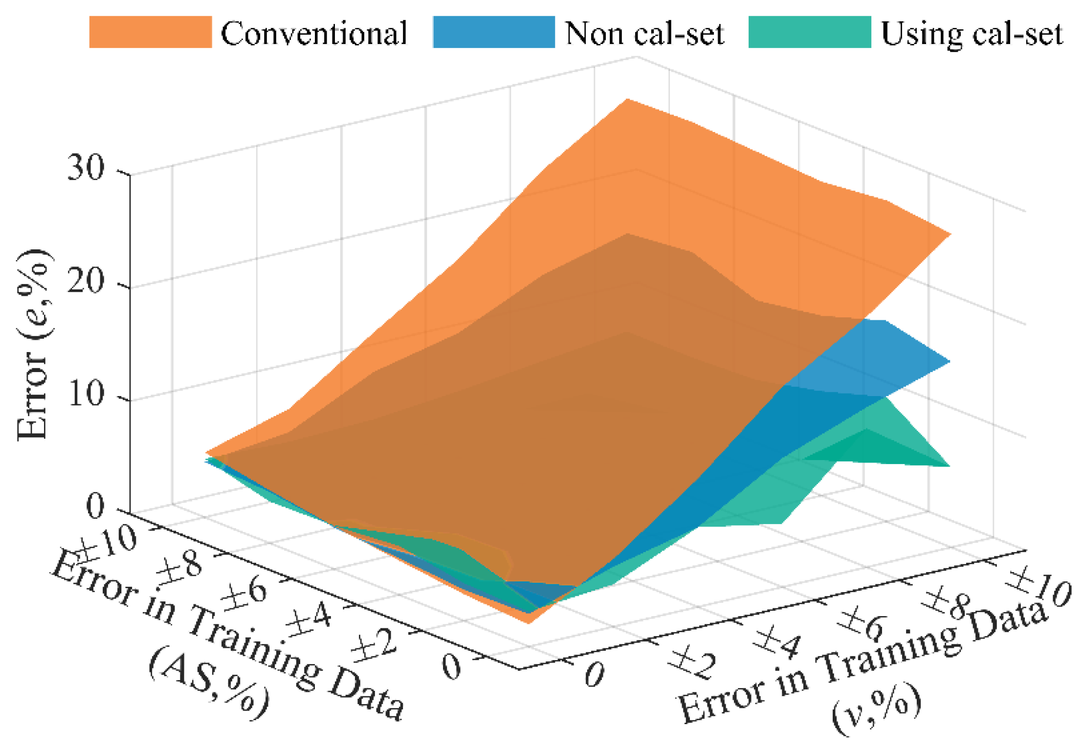
4.4. Influence of Overfitting in BwimNet and Solution
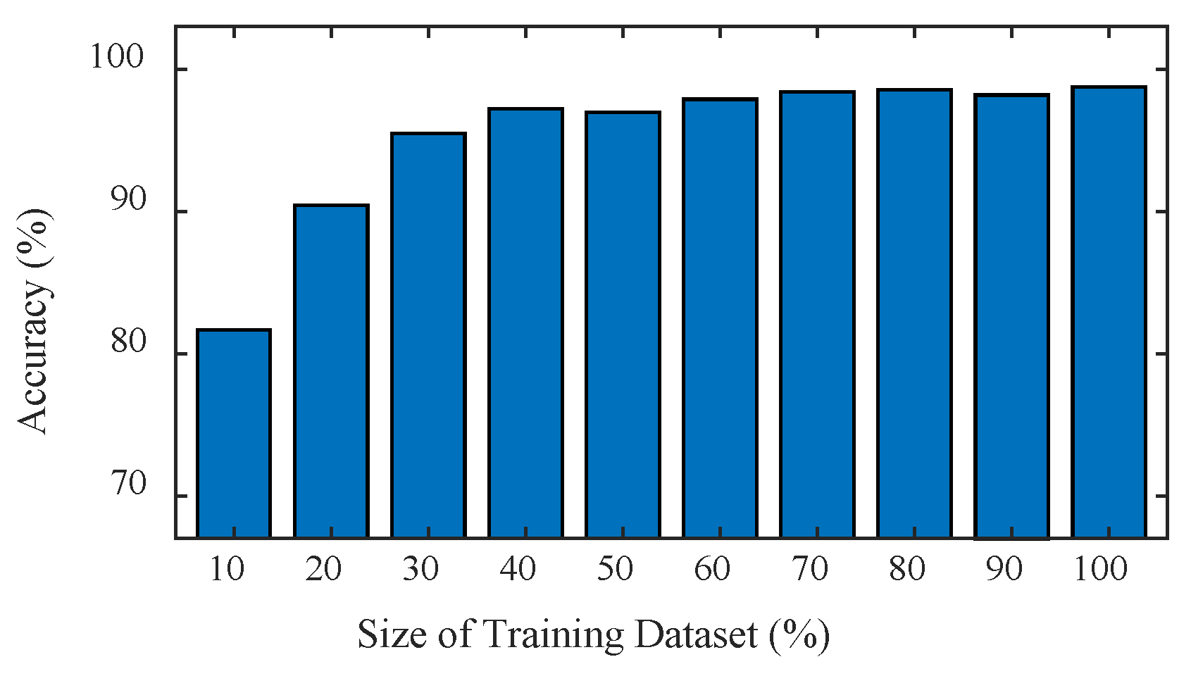
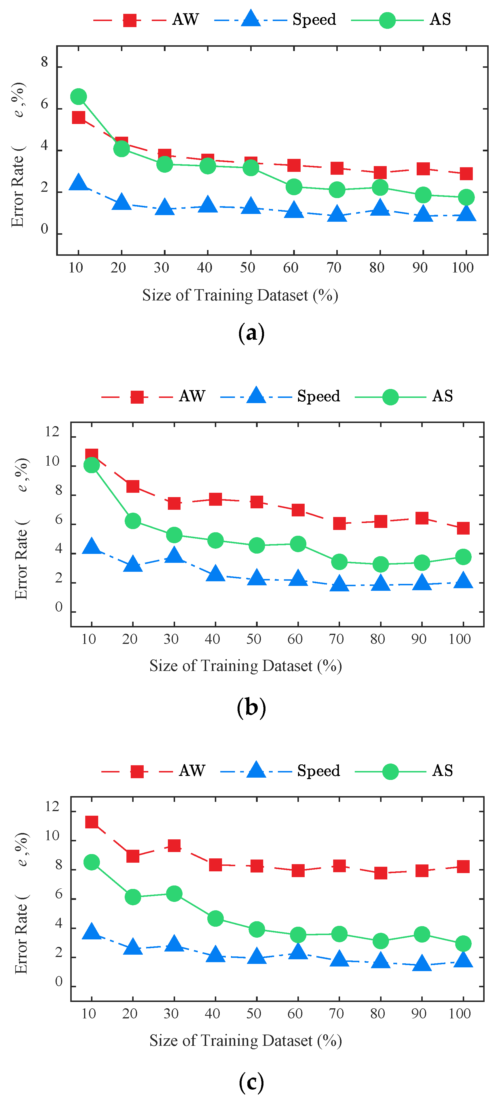
4.5. Effect of Size of Training Set
4.6. Effect of Lateral Position
5. Discussion
- (1)
- The BwimNet is found to be able to identify moving vehicles’ properties normally with polluted training data. Compared with the conventional method, the proposed method is much less sensitive to the errors in training data.
- (2)
- The weights of closely-spaced axles can also be predicted with acceptable accuracy, which can hardly be identified by conventional BWIMs under the considered cases. However, methods usually tend to perform better in numerical simulations than in field tests. Further study should be conducted to evaluate the proposed method in field application.
- (3)
- Accuracy of axle weight, axle spacing, and axle count rises with the increase of the dataset size at first and then tends to level off. The result shows that 4000 samples and 2800 samples might be sufficient for the training set of CNN-1 and CNN-2, respectively.
- (4)
- Although the identification error of the BwimNet method may slightly increase with the deterioration of road surface condition, this method still achieved acceptable identification accuracy.
6. Summary and Conclusions
Author Contributions
Funding
Acknowledgments
Conflicts of Interest
Appendix A

Appendix B
Appendix C

| Stage | Operation |
|---|---|
| 1. Data acquisition | a. Install one strain sensor under the soffit of each girder or slab of the target bridge for the purpose of obtaining bridge strain responses. b. Install (temporary) axle detectors (pressure sensitive sensors placed on top of the bridge, FAD sensors, or surveillance cameras) on the bridge. c. Collect training data with vehicle speed and axle spacings and relative bridge response. Then, uninstall the axle detectors if needed. d. Calculate the influence line from measured bridge response using the matrix method. |
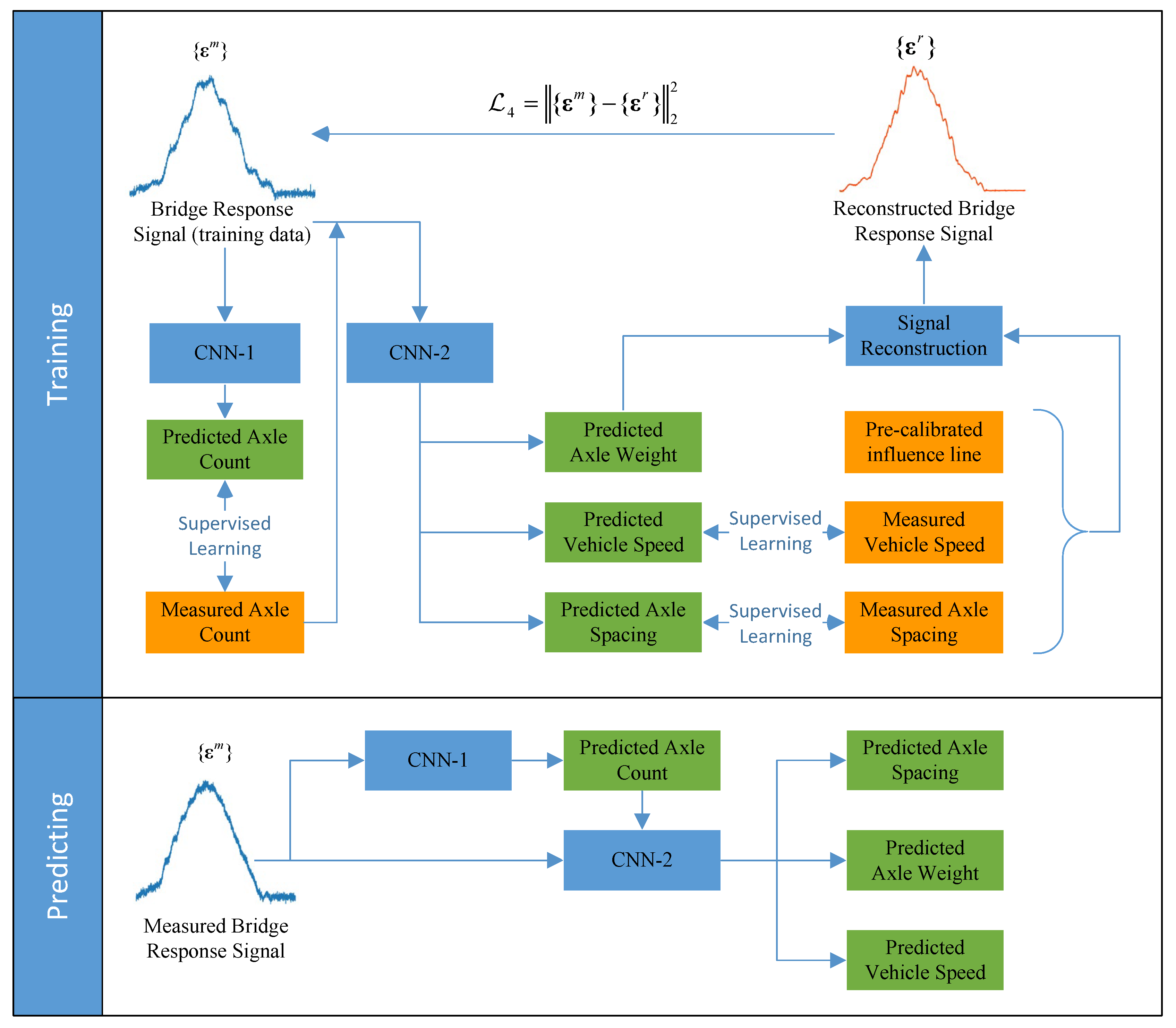
| 2. Network Training | e. Construct and train the CNN-1 network with bridge responses as input and axle counts as output (CNN-1 identifies the axle count of passing vehicles). f. Construct and train the CNN-2 network with axle count and true bridge responses as input, axle spacings, speed, and reconstructed bridge response as output. It should be noted that axle weights as output are the middle products of the signal reconstruction procedure in CNN-2. So, it does not need to provide weight information for the training process. |
| 3. Predicting | g. Acquire bridge responses under the travelling vehicle to be weighed by using strain sensors. Predict axle count of the vehicle by using CNN-1. Then, feed the strain response and axle count to CNN-2 and get estimations of speed, axle spacings, and axle weights of the vehicle. |
References
- Deng, L.; Bi, T.; He, W.; Wang, W. Vehicle weight limit analysis method for reinforced concrete bridges based on fatigue life. Cn. J. Highw. Transp 2017, 30, 72–78. [Google Scholar]
- Deng, L.; Duan, L.; He, W.; Ji, W. Study on vehicle model for vehicle-bridge coupling vibration of highway bridges in China. Cn. J. Highw. Transp. 2018, 31, 92–100. [Google Scholar]
- Lydon, M.; Taylor, S.E.; Robinson, D.; Mufti, A.; Brien, E.J.O. Recent developments in bridge weigh in motion (B-WIM). J. Civ. Struct. Heal. Monit. 2016, 6, 69–81. [Google Scholar] [CrossRef]
- Shokravi, H.; Shokravi, H.; Bakhary, N.; Heidarrezaei, M.; Koloor, S.S.R.; Petrů, M. Vehicle-assisted techniques for health monitoring of bridges. Sensors 2020, 20, 1–29. [Google Scholar] [CrossRef] [PubMed]
- Zhao, H.; Uddin, N.; Shao, X.; Zhu, P.; Tan, C. Field-calibrated influence lines for improved axle weight identification with a bridge weigh-in-motion system. Struct. Infrastruct. Eng. 2015, 11, 721–743. [Google Scholar] [CrossRef]
- OBrien, E.J.; Quilligan, M.J.; Karoumi, R. Calculating an influence line from direct measurements. Proc. Inst. Civ. Eng. Bridg. Eng. 2006, 159, 31–34. [Google Scholar] [CrossRef]
- Moses, F. Weigh-in-motion system using instrumented bridges. J. Transp. Eng. 1979, 105. [Google Scholar]
- O’Brien, E.J.; Znidaric, A.; Baumgärtner, W.; González, A.; McNulty, P. Weighing-In-Motion of Axles and Vehicles for Europe (WAVE) WP1. 2: Bridge WIM Systems; University College Dublin: Dublin, UK, 2001; ISBN 9619036611. [Google Scholar]
- Chatterjee, P.; OBrien, E.; Li, Y.; González, A. Wavelet domain analysis for identification of vehicle axles from bridge measurements. Comput. Struct. 2006, 84, 1792–1801. [Google Scholar] [CrossRef]
- Zhao, H.; Uddin, N.; O’Brien, E.J.; Shao, X.; Zhu, P. Identification of vehicular axle weights with a bridge weigh-in-motion system considering transverse distribution of wheel loads. J. Bridg. Eng. 2014, 19. [Google Scholar] [CrossRef]
- Kalin, J.; Žnidarič, A.; Lavrič, I. Practical Implementation of Nothing-on-the-Road Bridge Weigh-in-Motion System. In Proceedings of the International Symposium on Heavy Vehicle Weights and Dimensions, Pennsylvania University, University Park, PA, USA, 18–22 June 2006; pp. 3–10. [Google Scholar]
- Ieng, S.-S.; Zermane, A.; Schmidt, F.; Jacob, B. Analysis of B-WIM Signals Acquired in Millau Orthotropic Viaduct Using Statistical Classification. In Proceedings of the International on Weigh-In-Motion (ICWIM 6), Dallas, TX, USA, 4–7 June 2012; pp. 43–52. [Google Scholar]
- Venugopala, P.S.; Ashwini, B. Detection and classification of vehicles on curved roads. Int. J. Innov. Technol. Explor. Eng. 2019, 8, 152–156. [Google Scholar] [CrossRef]
- Zhang, Z.; Tan, T.; Huang, K.; Wang, Y. Three-dimensional deformable-model-based localization and recognition of road vehicles. IEEE Trans. Image Process. 2012, 21, 1–13. [Google Scholar] [CrossRef] [PubMed]
- Kawakatsu, T.; Kakitani, A.; Aihara, K.; Takasu, A.; Adachi, J. Traffic surveillance system for bridge vibration analysis. In Proceedings of the IEEE International Conference on Information Reuse and Integration, San Diego, CA, USA, 4–6 August 2017; pp. 69–74. [Google Scholar] [CrossRef]
- Ojio, T.; Carey, C.H.; OBrien, E.J.; Doherty, C.; Taylor, S.E. Contactless Bridge Weigh-in-Motion. J. Bridg. Eng. 2016, 21, 1–11. [Google Scholar] [CrossRef]
- Kawakatsu, T.; Aihara, K.; Takasu, A.; Adachi, J. Deep Sensing Approach to Single-Sensor Vehicle Weighing System on Bridges. IEEE Sens. J. 2019, 19, 253–256. [Google Scholar] [CrossRef]
- He, W.; Deng, L.; Shi, H.; Cai, C.S.; Yu, Y. Novel Virtual Simply Supported Beam Method for Detecting the Speed and Axles of Moving Vehicles on Bridges. J. Bridg. Eng. 2017, 22, 1–16. [Google Scholar] [CrossRef]
- Deng, L.; He, W.; Yu, Y.; Cai, C.S. Equivalent Shear Force Method for Detecting the Speed and Axles of Moving Vehicles on Bridges. J. Bridg. Eng. 2018, 23, 1–13. [Google Scholar] [CrossRef]
- Kalhori, H.; Makki Alamdari, M.; Zhu, X.; Samali, B.; Mustapha, S. Non-intrusive schemes for speed and axle identification in bridge-weigh-in-motion systems. Meas. Sci. Technol. 2017, 28. [Google Scholar] [CrossRef]
- Yu, Y.; Cai, C.S.; Deng, L. Vehicle axle identification using wavelet analysis of bridge global responses. JVC J. Vib. Control 2017, 23, 2830–2840. [Google Scholar] [CrossRef]
- Kawakatsu, T.; Kinoshita, A.; Aihara, K.; Takasu, A.; Adachi, J. Deep sensing approach to single-sensor bridge weighing in motion. In Proceedings of the 9th European Workshop on Structural Health Monitoring (EWSHM 2018), Manchester, UK, 10–13 July 2018; pp. 1–12. [Google Scholar]
- LeCun, Y.; Boser, B.; Denker, J.S.; Henderson, D.; Howard, R.E.; Hubbard, W.; Jackel, L.D. Backpropagation applied to handwritten zip code recognition. Neural Comput. 1989, 1, 541–551. [Google Scholar] [CrossRef]
- Hornik, K.; Stinchcombe, M.; White, H. Multilayer feedforward networks are universal approximators. Neural Netw. 1989, 2, 359–366. [Google Scholar] [CrossRef]
- González, A.; Papagiannakis, A.T.; O’Brien, E.J. Evaluation of an Artificial Neural Network Technique Applied to Multiple-Sensor Weigh-in-Motion Systems. Transp. Res. Rec. 2003, 151–159. [Google Scholar] [CrossRef]
- Kim, S.; Lee, J.; Park, M.S.; Jo, B.W. Vehicle signal analysis using artificial neural networks for a Bridge Weigh-in-Motion system. Sensors 2009, 9, 7943–7956. [Google Scholar] [CrossRef] [PubMed]
- Kawakatsu, T.; Aihara, K.; Takasu, A.; Adachi, J. Fully-Neural Approach to Heavy Vehicle Detection on Bridges Using a Single Strain Sensor. In Proceedings of the International Conference on Acoustics, Speech and Signal Processing (ICASSP), Barcelona, Spain, 4–9 May 2020; pp. 3047–3051. [Google Scholar] [CrossRef]
- LeCun, Y.; Bottou, L.; Bengio, Y.; Haffner, P. Gradient-based learning applied to document recognition. Proc. IEEE 1998, 86, 2278–2324. [Google Scholar] [CrossRef]
- Redmon, J.; Divvala, S.; Girshick, R.; Farhadi, A. You only look once: Unified, real-time object detection. In Proceedings of the IEEE Computer Society Conference on Computer Vision and Pattern Recognition (CVPR), Las Vegas, NV, USA, 27–30 June 2016; pp. 779–788. [Google Scholar] [CrossRef]
- Sangeetha, V.; Prasad, K.J.R. Syntheses of novel derivatives of 2-acetylfuro[2,3-a]carbazoles, benzo[1,2-b]-1,4-thiazepino[2,3-a]carbazoles and 1-acetyloxycarbazole-2- carbaldehydes. Ind. J. Chem. 2006, 45, 1951–1954. [Google Scholar] [CrossRef]
- Ren, S.; He, K.; Girshick, R.; Sun, J. Faster r-cnn: Towards real-time object detection with region proposal networks. In Proceedings of the Advances in Neural Information Processing Systems, Montreal, Canada, 7–10 December 2015; pp. 91–99. [Google Scholar]
- Krizhevsky, A.; Sutskever, I.; Hinton, G.E. Imagenet classification with deep convolutional neural networks. In Proceedings of the 25th International Conference on Neural Information Processing Systems (NIPS), Lake Tahoe, NV, USA, 3–6 December 2012; Volume 1, pp. 1097–1105. [Google Scholar]
- Bao, Y.; Chen, Z.; Wei, S.; Xu, Y.; Tang, Z.; Li, H. The State of the Art of Data Science and Engineering in Structural Health Monitoring. Engineering 2019, 5, 234–242. [Google Scholar] [CrossRef]
- Hinton, G.E.; Salakhutdinov, R.R. Reducing the dimensionality of data with neural networks. Science 2006, 313, 504–507. [Google Scholar] [CrossRef] [PubMed]
- Zhang, S.; Yao, Y.; Hu, J.; Zhao, Y.; Li, S.; Hu, J. Deep autoencoder neural networks for short-term traffic congestion prediction of transportation networks. Sensors 2019, 19, 1–19. [Google Scholar] [CrossRef]
- Li, X.; Zhang, L.; Zhang, J. State-of-the-art review and trend of studies on coupling vibration for vehicle and highway bridge system. Eng. Mech. 2008, 3, 230–240. [Google Scholar]
- Cai, C.S.; Shi, X.; Araujo, M.S.; Chen, S. Influence of approach span conditions on vehicle-induced dynamic response of slab-on-girder bridges: Field and numerical simulations. In Proceedings of the Transportation Research Board 86th Annual Meeting, Washington DC, USA, 21–25 January 2007. [Google Scholar]
- Deng, L.; Cai, C.S. Identification of dynamic vehicular axle loads: Demonstration by a field study. JVC J. Vib. Control 2011, 17, 183–195. [Google Scholar] [CrossRef]
- Deng, L.; Cai, C.S. Identification of dynamic vehicular axle loads: Theory and simulations. JVC J. Vib. Control 2010, 16, 2167–2194. [Google Scholar] [CrossRef]
- Yang, Y.B.; Lin, C.W. Vehicle-bridge interaction dynamics and potential applications. J. Sound Vib. 2005, 284, 205–226. [Google Scholar] [CrossRef]
- Deng, L.; He, W.; Yu, Y.; Wang, W. Research progress in theory and applications of highway vehicle-bridge coupling vibration. Cn. J. Highw. Transp. 2018, 31, 38–54. [Google Scholar]
- Dodds, C.J.; Robson, J.D. The description of road surface roughness. J. Sound Vib. 1973, 31, 175–183. [Google Scholar] [CrossRef]
- Huang, D.; Wang, T. Lo Impact analysis of cable-stayed bridges. Comput. Struct. 1992, 43, 897–908. [Google Scholar] [CrossRef]
- International Organization for Standardization (ISO) Mechanical Vibration-Road Surface Profiles-Reporting of Measured Data; International Organization for Standardization (ISO): Geneva, Switzerland, 1995.
- Deng, L.; Cai, C.S. Identification of parameters of vehicles moving on bridges. Eng. Struct. 2009, 31, 2474–2485. [Google Scholar] [CrossRef]
- Deng, L.; Cai, C.S. Development of dynamic impact factor for performance evaluation of existing multi-girder concrete bridges. Eng. Struct. 2010, 32, 21–31. [Google Scholar] [CrossRef]
- Harris, N.K.; OBrien, E.J.; González, A. Reduction of bridge dynamic amplification through adjustment of vehicle suspension damping. J. Sound Vib. 2007, 302, 471–485. [Google Scholar] [CrossRef]
- Miao, T.J.; Chan, T.H.T. Bridge live load models from WIM data. Eng. Struct. 2002, 24, 1071–1084. [Google Scholar] [CrossRef]
- Sun, S.; Sun, L. Statistic model of vehicle loads for highway bridges. J. Tongji Univ. 2012, 40, 198–204. [Google Scholar] [CrossRef]
- Shi, X.M.; Cai, C.S. Simulation of dynamic effects of vehicles on pavement using a 3D interaction model. J. Transp. Eng. 2009, 135, 736–744. [Google Scholar] [CrossRef]
- American Association of State Highway and Transportation Officials (AASHTO) Standard specifications for highway bridges; American Association of State Highway and Transportation Officials (AASHTO): Washington, DC, USA, 2002.
- Rowley, C.; Gonzalez, A.; O’Brien, E.; Znidaric, A. Comparison of conventional and regularized bridge weigh-in-motion algorithms. In Proceedings of the International Conference on Heavy Vehicles, Paris, France, 19–22 May 2008; pp. 19–22. [Google Scholar]
- O’Brien, E.J.; Rowley, C.W.; González, A.; Green, M.F. A regularised solution to the bridge weigh-in-motion equations. Int. J. Heavy Veh. Syst. 2009, 16, 310–327. [Google Scholar] [CrossRef]
- Yu, Y.; Deng, L.; Wang, W.; Cai, C.S. Local impact analysis for deck slabs of prestressed concrete box-girder bridges subject to vehicle loading. JVC J. Vib. Control 2017, 23, 31–45. [Google Scholar] [CrossRef]


| Input: |
|---|
| , time-history of measured strain response |
| I(x), influence line of bridge response |
| Output: |
| N, axle count of vehicle v, velocity of vehicle d, vector of axle spacing (AS) , rebuilt strain response |
| By-products: |
| F, vector of axle weight (AW) GVW, gross vehicle weight |
| Truck Model | Configuration | ||||||||
|---|---|---|---|---|---|---|---|---|---|
| Axle Weight (kN) | Axle Spacing (m) | ||||||||
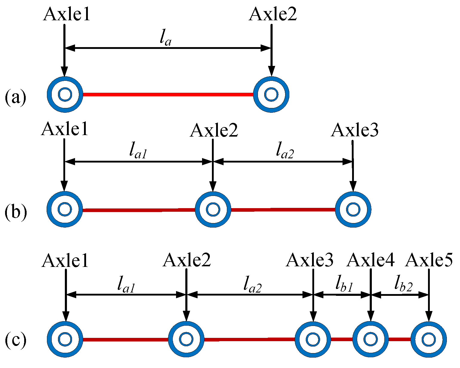
| Axle1 | Axle2 | Axle3 | Axle4 | Axle5 | la1 | la2 | lb1 | lb2 | |
| Two-axle truck | 43.60 | 29.90 | - | - | - | 7.90 | |||
| Three-axle truck | 35.60 | 142.10 | 142.40 | - | - | 4.27 | 4.27 | - | - |
| Five-axle truck | 56.70 | 117.00 | 76.40 | 72.90 | 69.40 | 3.00 | 5.10 | 1.10 | 1.10 |
| Truck | Method | Relative Error (%) | |||||
|---|---|---|---|---|---|---|---|
| AW1 | AW2 | AW3 | AW4 | AW5 | GVW | ||
| Two-axle truck | Moses’ algorithm | 1.72 | 2.17 | - | - | - | 0.40 |
| BwimNet | 2.27 | 3.51 | - | - | - | 0.61 | |
| Three-axle truck | Moses’ algorithm | 4.16 | 3.26 | 1.96 | - | - | 0.32 |
| BwimNet | 6.64 | 6.29 | 4.56 | - | - | 1.48 | |
| Five-axle truck | Moses’ algorithm | 4.70 | 7.46 | 48.03 | 79.04 | 40.25 | 0.27 |
| BwimNet | 7.55 | 5.76 | 10.62 | 11.86 | 5.76 | 1.30 | |
| Truck | Relative Error (%) | |||||
|---|---|---|---|---|---|---|
| AW1 | AW2 | AW3 | AW4 | AW5 | GVW | |
| Two-axle truck | 2.28 | 3.00 | - | - | - | 0.65 |
| Three-axle truck | 5.11 | 4.61 | 3.99 | - | - | 1.03 |
| Five-axle truck | 4.97 | 5.66 | 8.89 | 6.90 | 6.18 | 1.26 |
Publisher’s Note: MDPI stays neutral with regard to jurisdictional claims in published maps and institutional affiliations. |
© 2020 by the authors. Licensee MDPI, Basel, Switzerland. This article is an open access article distributed under the terms and conditions of the Creative Commons Attribution (CC BY) license (http://creativecommons.org/licenses/by/4.0/).
Share and Cite
Wu, Y.; Deng, L.; He, W. BwimNet: A Novel Method for Identifying Moving Vehicles Utilizing a Modified Encoder-Decoder Architecture. Sensors 2020, 20, 7170. https://doi.org/10.3390/s20247170
Wu Y, Deng L, He W. BwimNet: A Novel Method for Identifying Moving Vehicles Utilizing a Modified Encoder-Decoder Architecture. Sensors. 2020; 20(24):7170. https://doi.org/10.3390/s20247170
Chicago/Turabian StyleWu, Yuhan, Lu Deng, and Wei He. 2020. "BwimNet: A Novel Method for Identifying Moving Vehicles Utilizing a Modified Encoder-Decoder Architecture" Sensors 20, no. 24: 7170. https://doi.org/10.3390/s20247170
APA StyleWu, Y., Deng, L., & He, W. (2020). BwimNet: A Novel Method for Identifying Moving Vehicles Utilizing a Modified Encoder-Decoder Architecture. Sensors, 20(24), 7170. https://doi.org/10.3390/s20247170