Pre-Trained Deep Convolutional Neural Network for Clostridioides Difficile Bacteria Cytotoxicity Classification Based on Fluorescence Images

 ,
,  ,
,  , and
, and
Abstract
1. Introduction
- proposing a solution for cell classification of fluorescence images based on the CNN models, which—thanks to using data augmentation and transfer learning—yielded satisfactory results even for a limited amount of data (we deployed and compared four pre-trained CNN architectures, including VGG-19, ResNet50, Xception, and DenseNet121 with an adjusted, densely connected classifier),
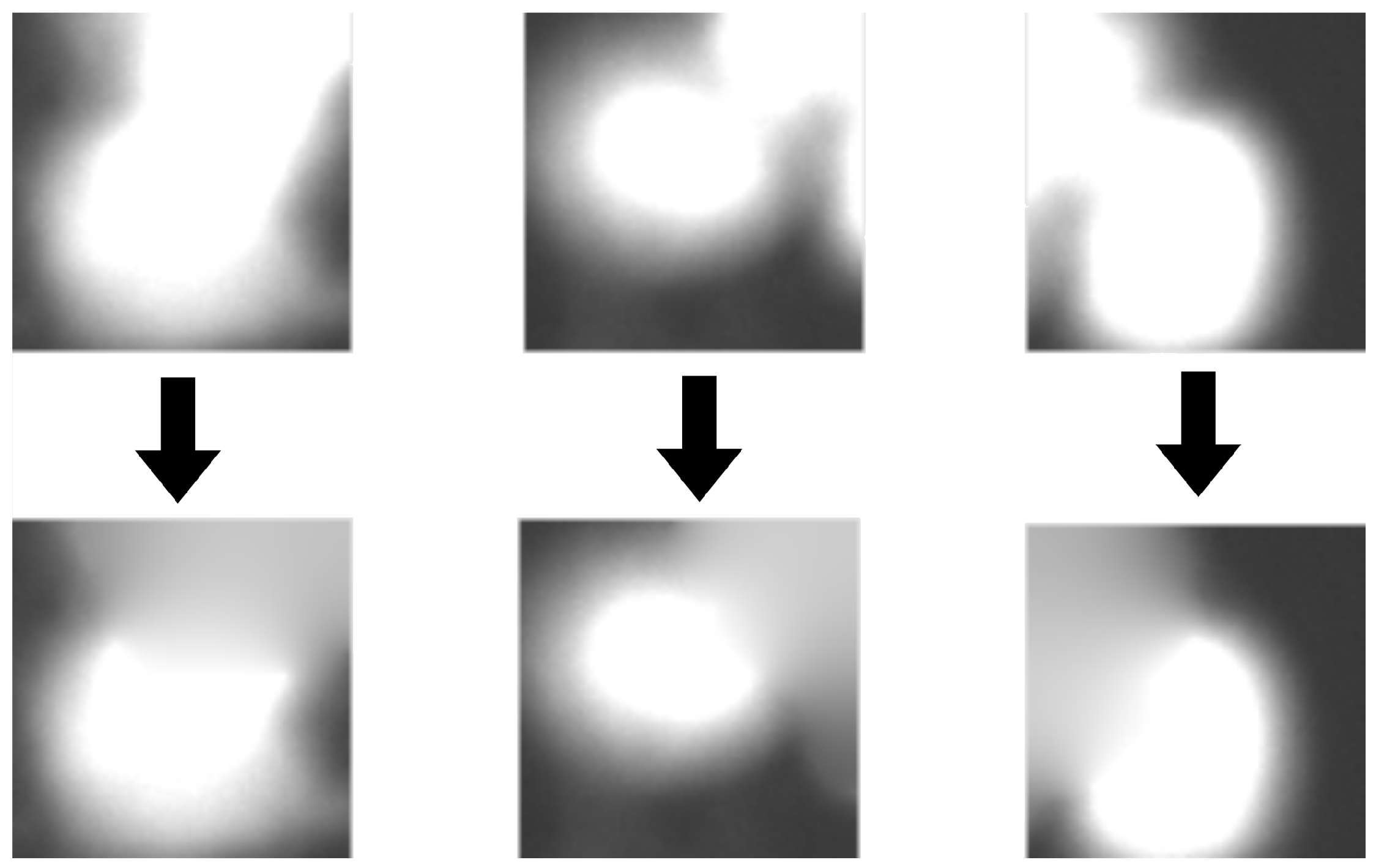
- removing unnecessary objects from the background of the image by an inpainting technique,
- training the network on different types of images and adding regularization in order both to make the model resistant to cell staining deviations and to avoid the overfitting problem.
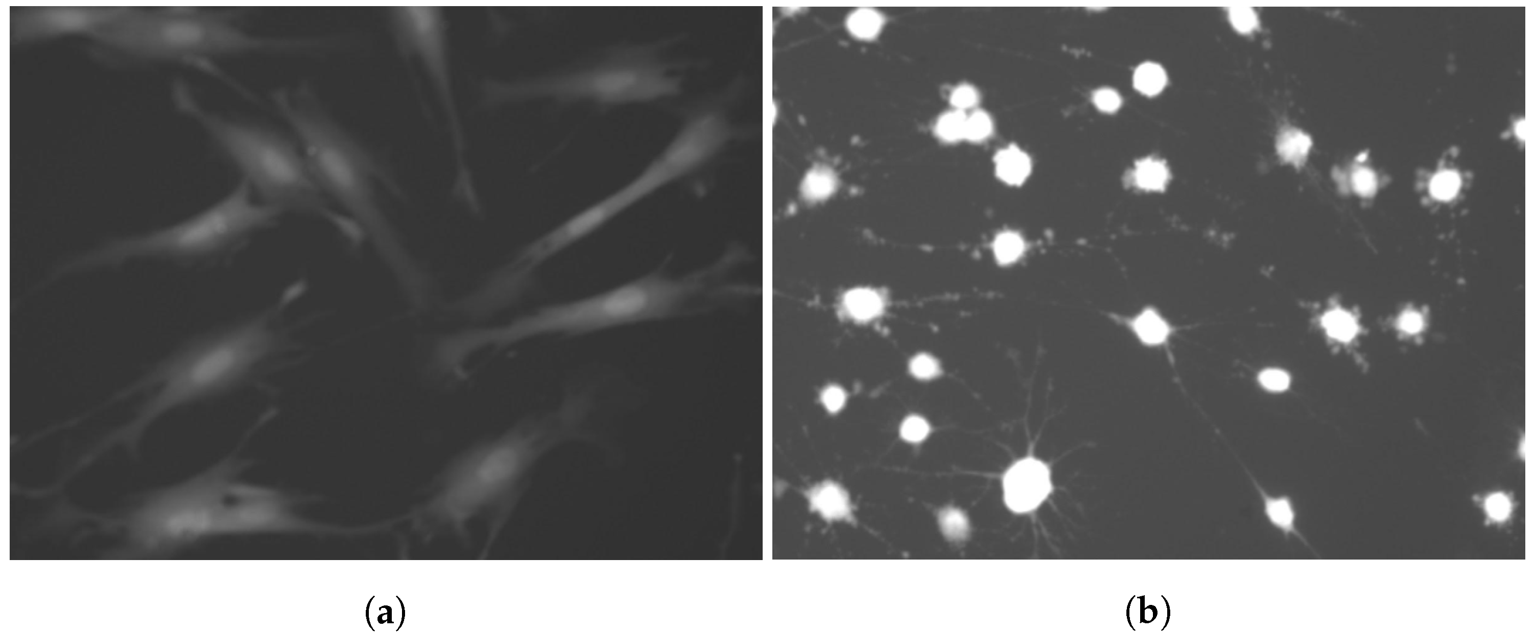
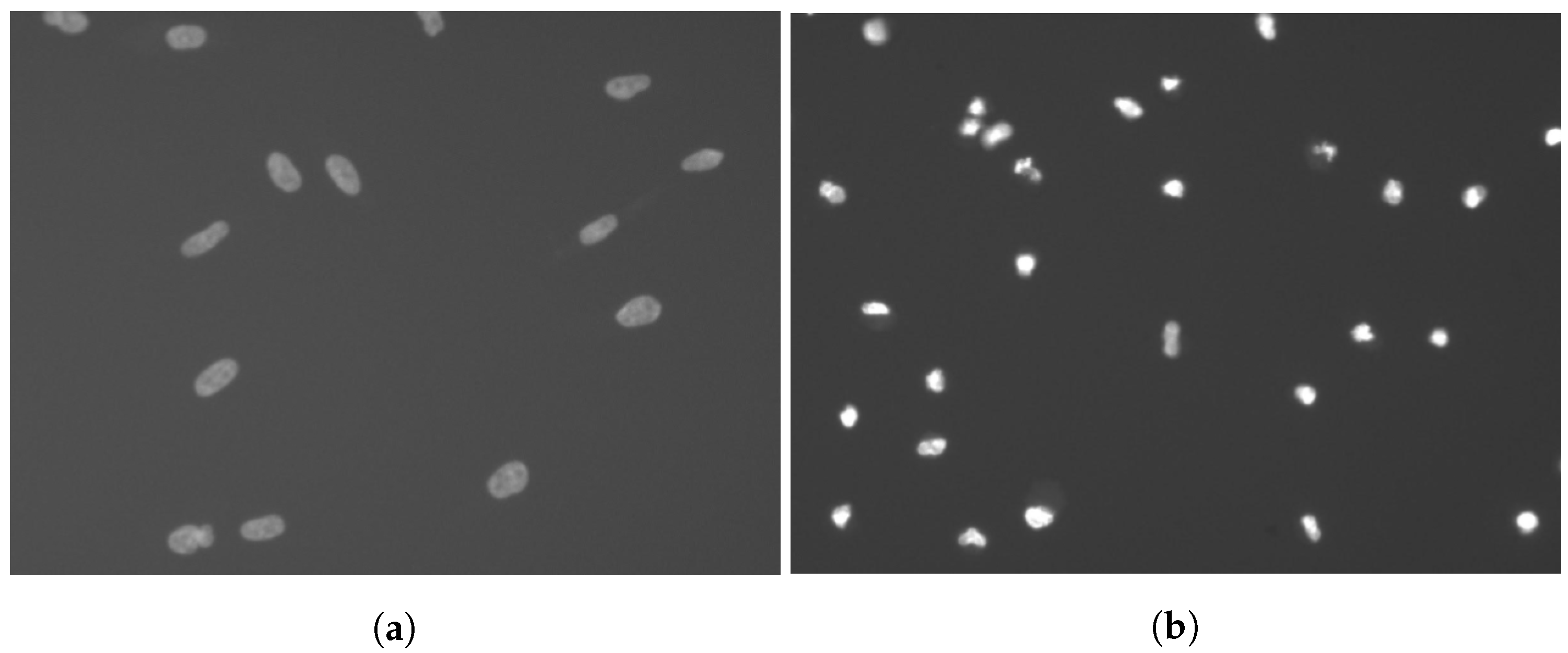
1.1. Fluorescence Images
1.2. Related Works
2. Methods
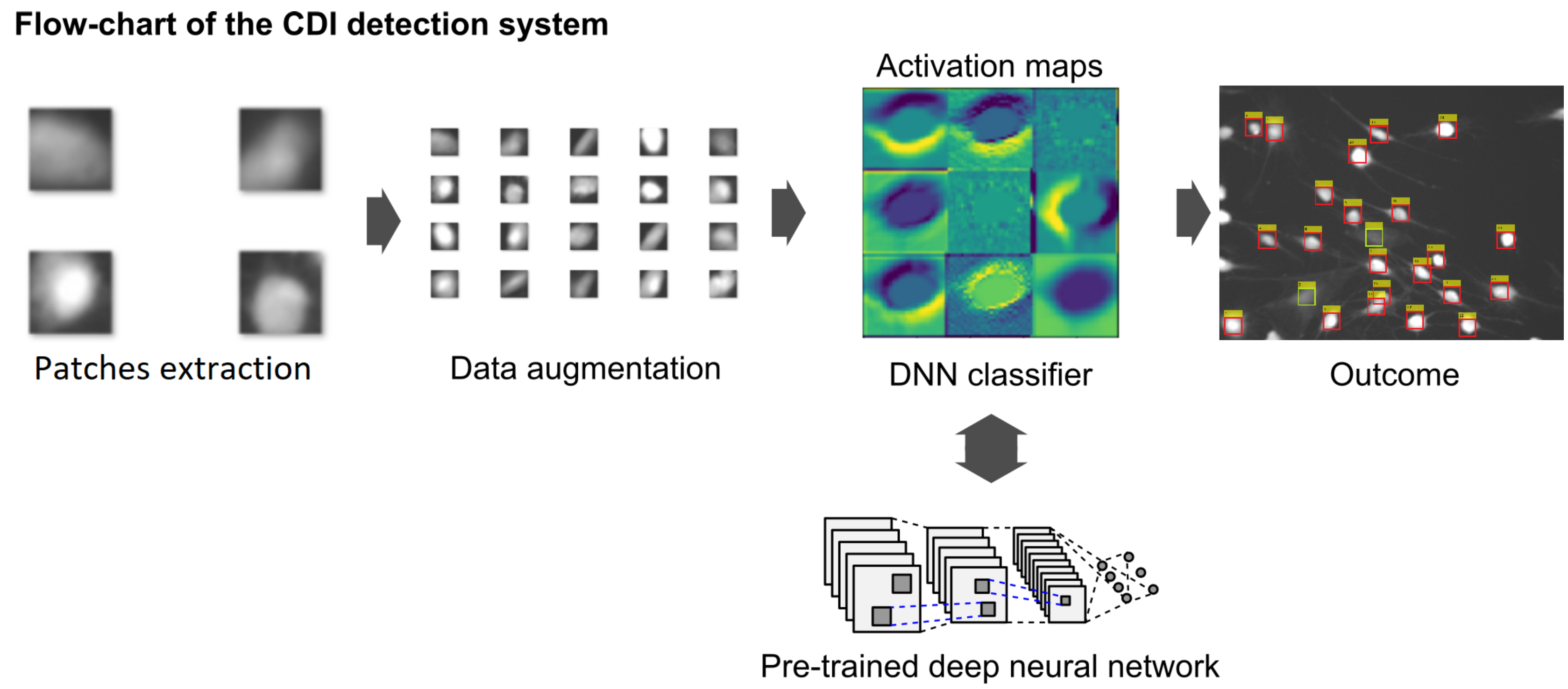
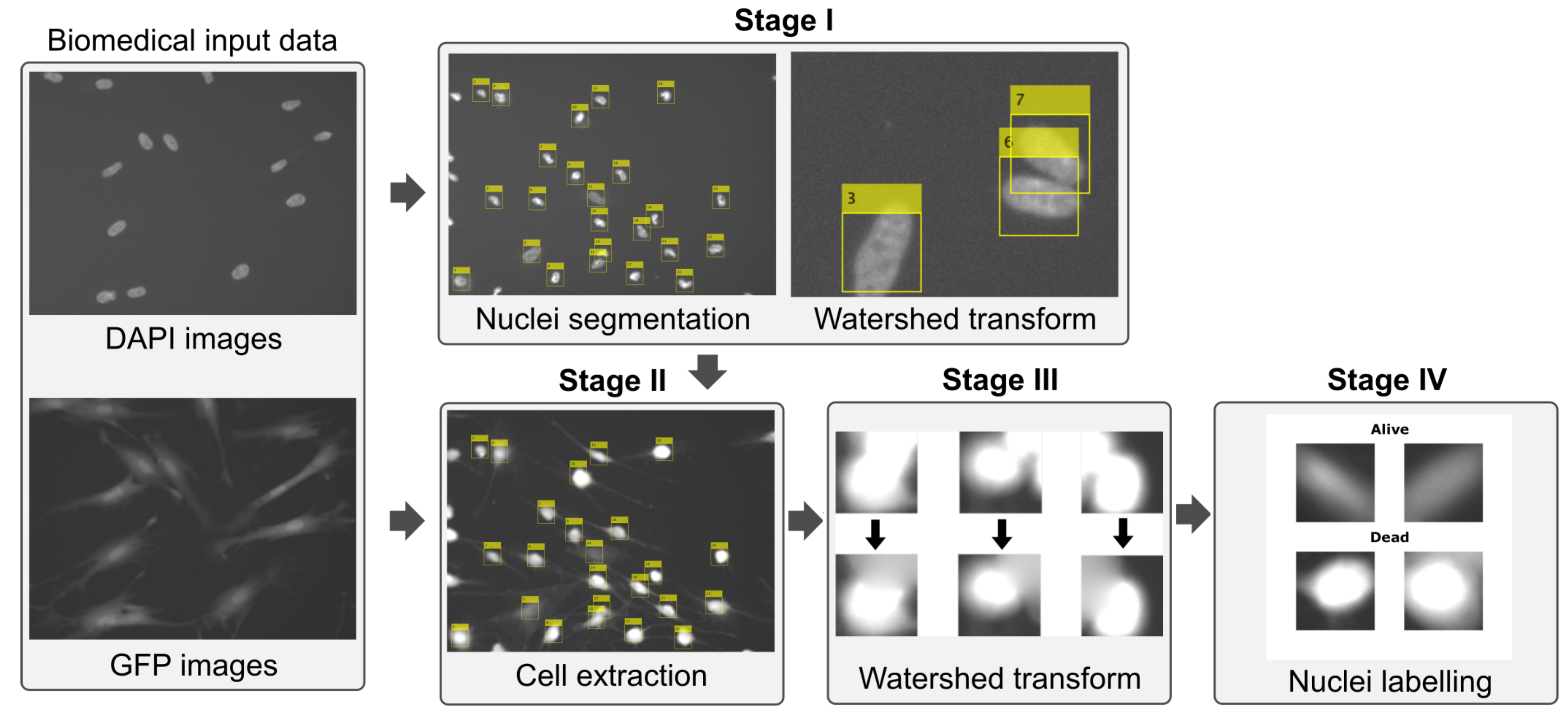
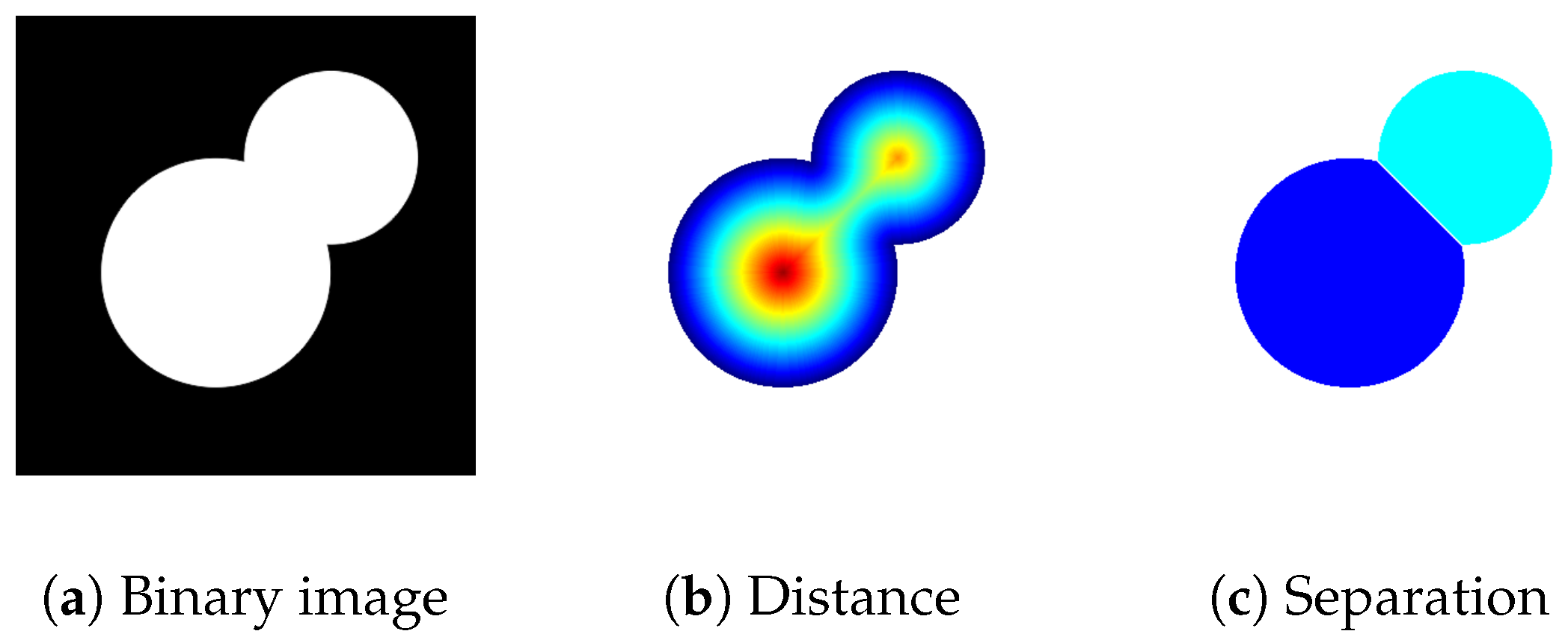
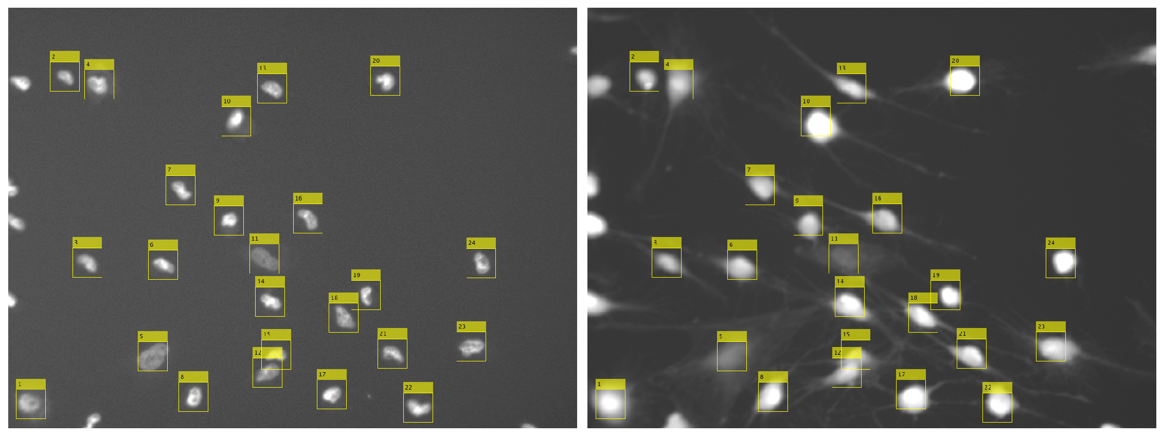
2.1. Cell Detection
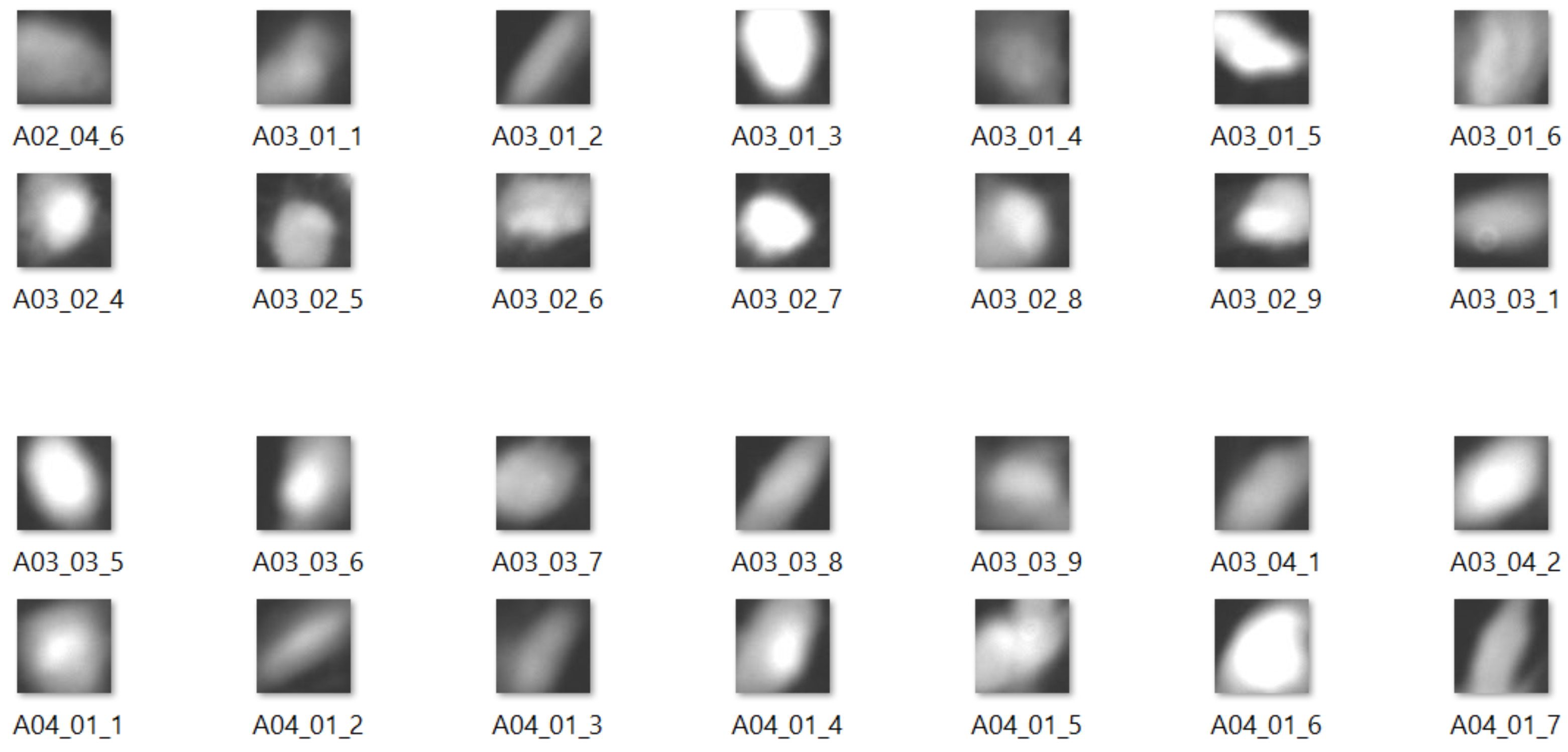
2.2. Dataset Augmentation
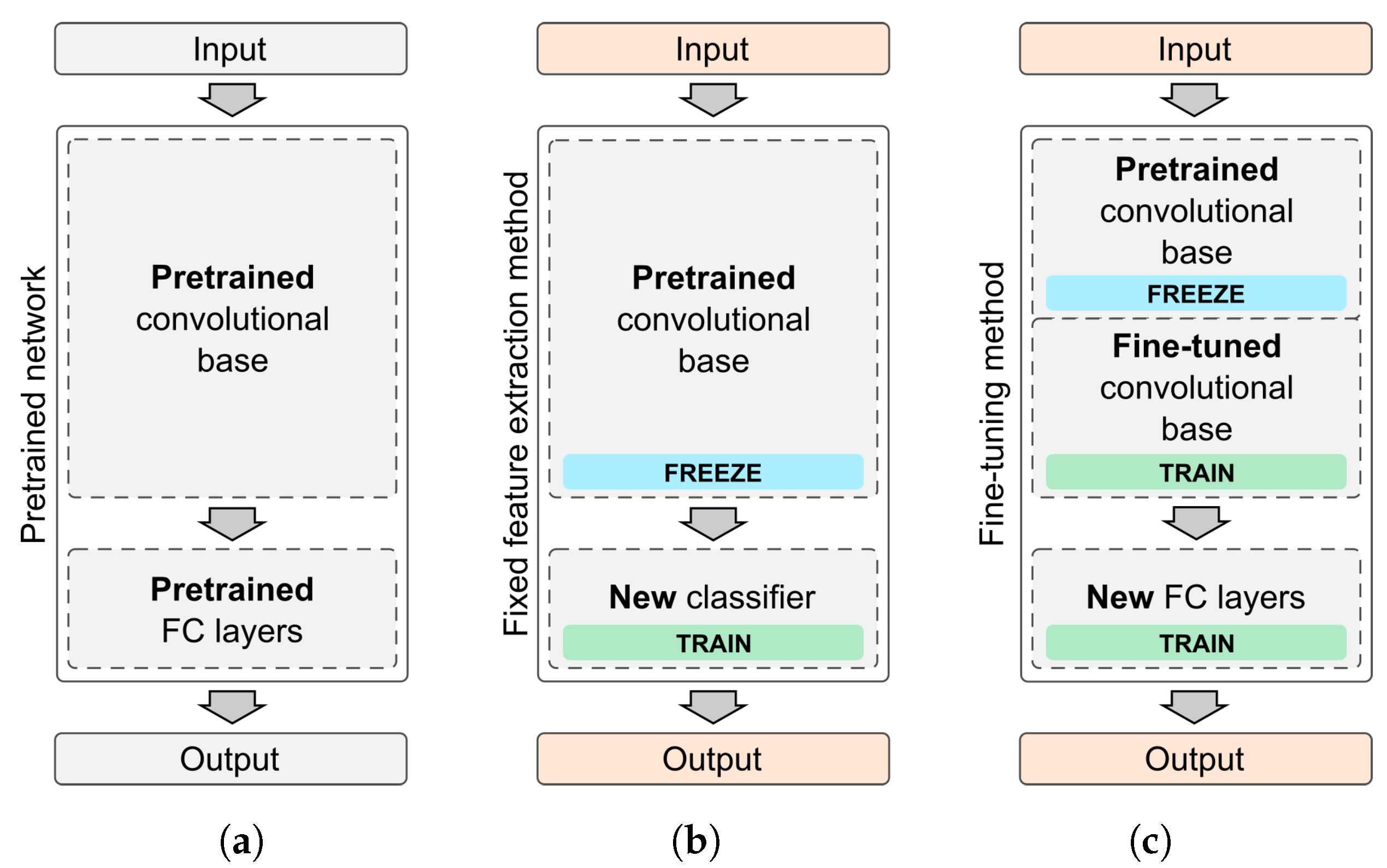
2.3. Deep Neural Networks with Transfer Learning
- Train the entire model—use the implemented architecture of the pre-trained model and train it on your dataset. Instead of using random weights, start from values of a pre-trained model.
- Feature extraction (freezing CNN model base)—train a new classifier on top of the pre-trained base model. The weights of convolution layers are left unchanged and only the last, fully connected layer is trained.
- Fine-tuning (training also some convolution layers)—retrain one or more convolution layers in addition to a fully connected classifier. Original convolution layer weights are used as starting points. Unlocked convolution layers are only tuned to a new problem.
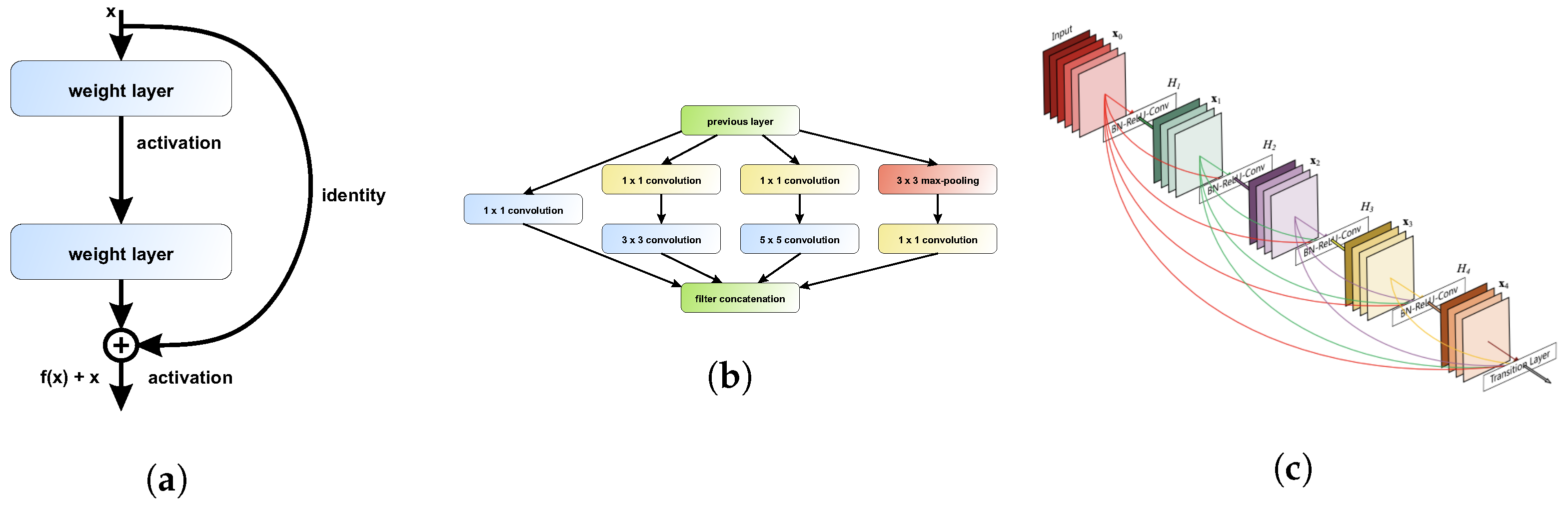
2.4. Pre-Trained Deep Learning Architectures
2.5. Parameter Selection
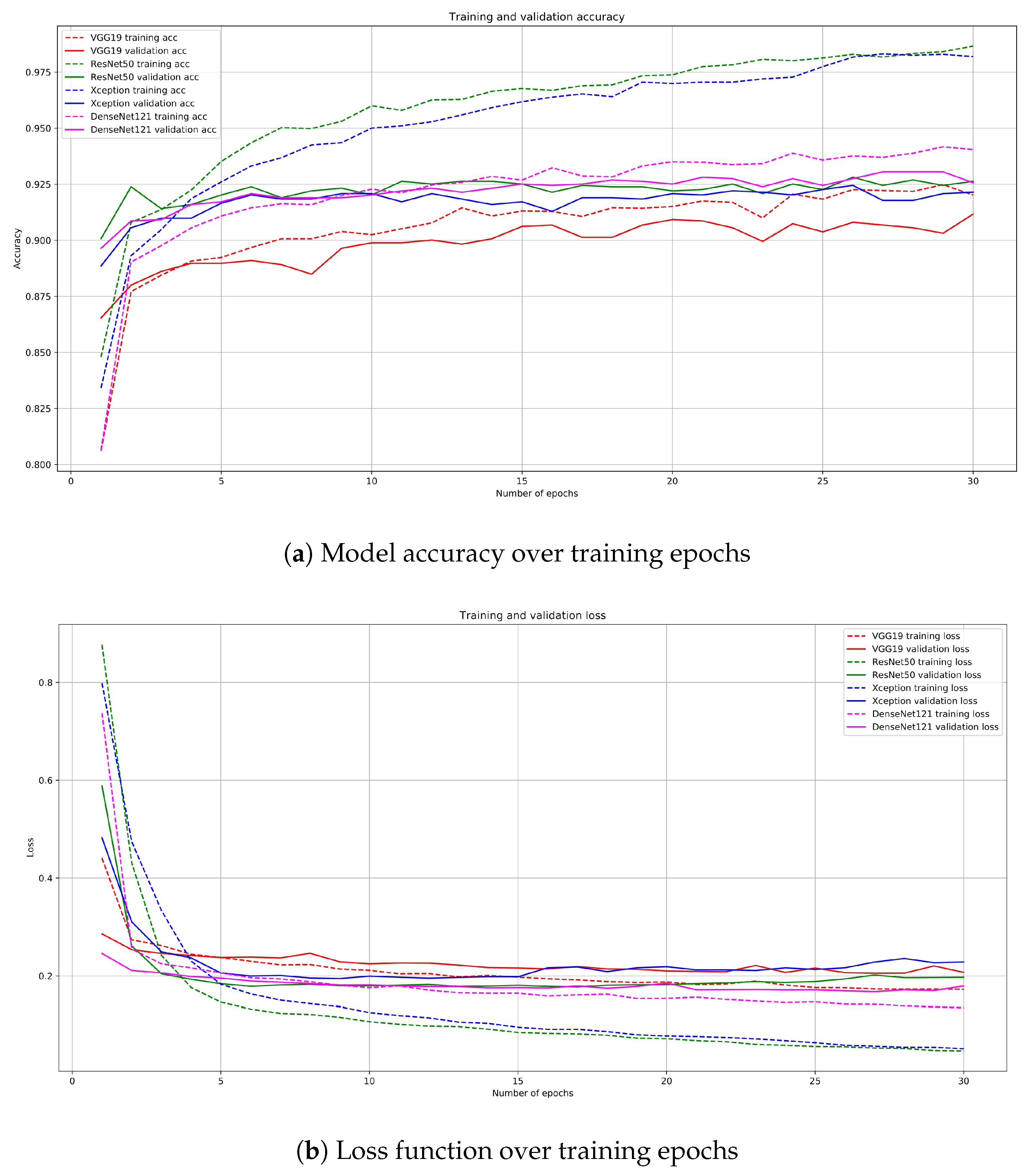
3. Results
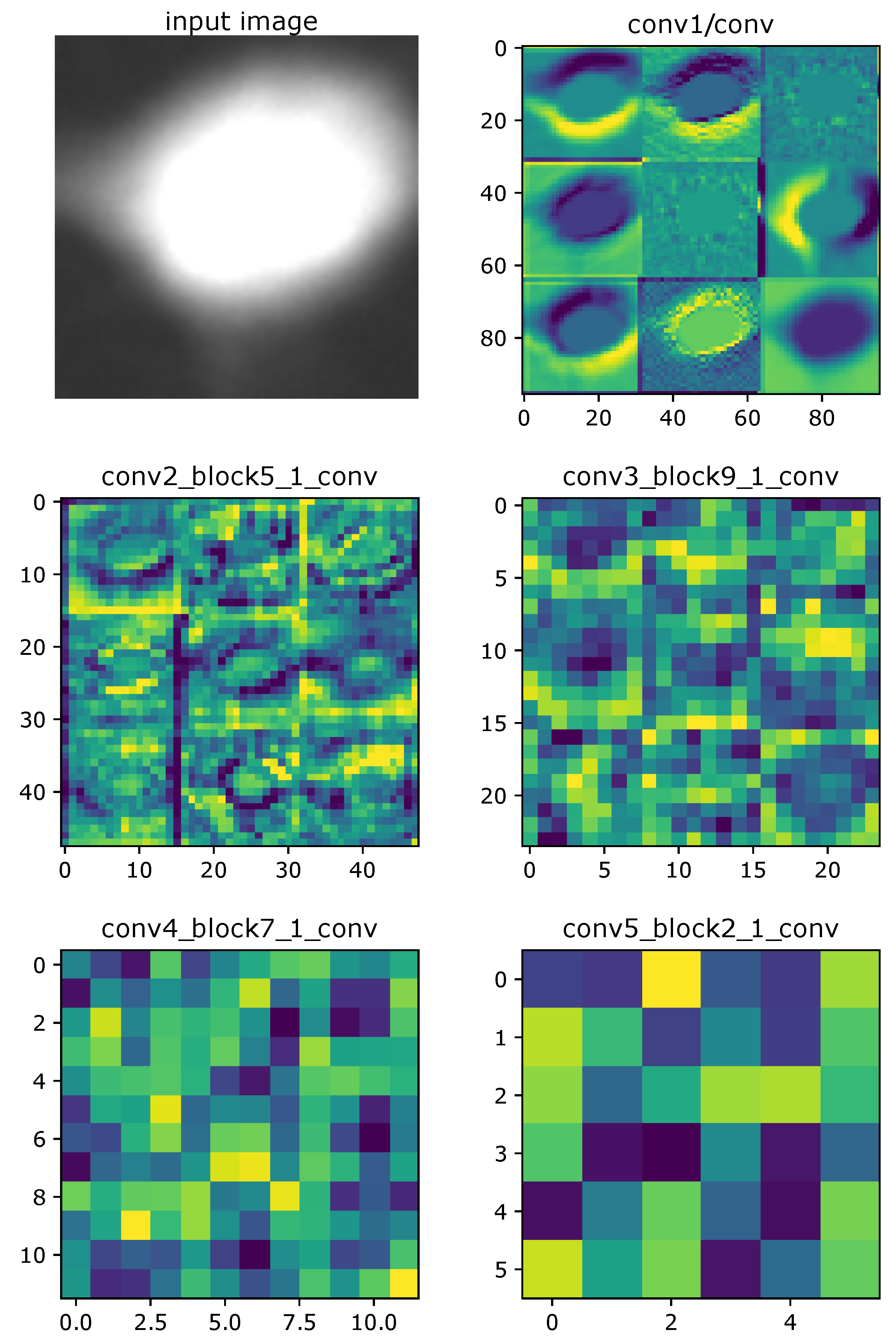
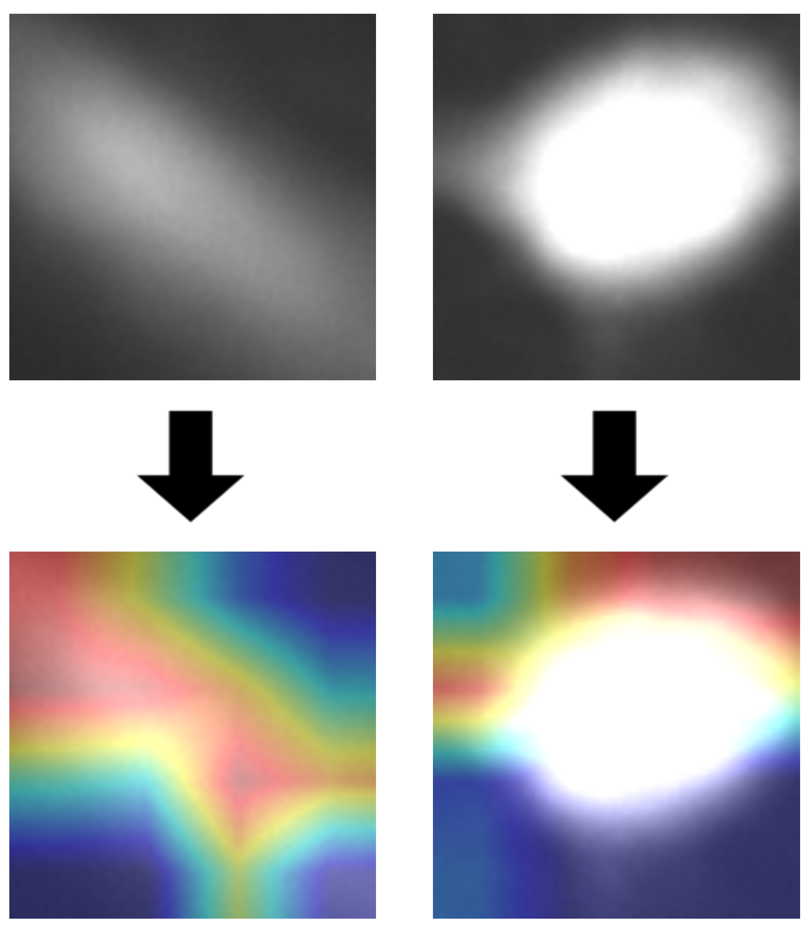
3.1. Visualization of the Convolutional Layers
3.2. Statistical Analysis
3.3. Comparison with Other Research Works
4. Conclusions and Discussions
Future Work
Author Contributions
Funding
Conflicts of Interest
References
- Smits, W.K.; Lyras, D.; Lacy, D.B.; Wilcox, M.H. Clostridium difficile infection. Nat. Rev. Dis. Prim. 2016, 2. [Google Scholar] [CrossRef] [PubMed]
- Czepiel, J.; Dróżdż, M.; Pituch, H.; Kuijper, E.J.; Perucki, W.; Mielimonka, A.; Goldman, S.; Wultańska, D.; Garlicki, A.; Biesiada, G. Clostridium difficile infection: Review. Eur. J. Clin. Microbiol. Infect. Dis. 2010, 38. [Google Scholar] [CrossRef]
- Reveles, K.R.; Lee, G.C.; Boyd, N.K.; Frei, C.R. The rise in Clostridium difficile infection incidence among hospitalized adults in the United States: 2001–2010. Am. J. Infect. Control 2014, 42, 1028–1032. [Google Scholar] [CrossRef] [PubMed]
- Centers for Disease Control and Prevention. QuickStats: Rates of Clostridium Difficile Infection among Hospitalized Patients Aged 65 Years, Age Group—National Hospital Discharge Survey, 1996–2009. MMWR Morb. Mortal. Wkly. Rep. 2011, 60, 1171. [Google Scholar]
- Lessa, F.C.; Gould, C.V.; McDonald, L.C. Current Status of Clostridium difficile Infection Epidemiology. Clin. Infect. Dis. 2012, 55, S65–S70. [Google Scholar] [CrossRef] [PubMed]
- Butler, M.; Olson, A.; Drekonja, D.M.; Shaukat, A.; Schwehr, N.A.; Shippee, N.D.; Wilt, T.J. Early Diagnosis, Prevention, and Treatment of Clostridium Difficile: Update; NCBI 5600 Fishers Lane: Rockville, MD, USA, 2016. [Google Scholar]
- Lessa, F.C.; Mu, Y.; Bamberg, W.M.; Beldavs, Z.G.; Dumyati, G.K.; Dunn, J.R.; Farley, M.M.; Holzbauer, S.M.; Meek, J.I.; Phipps, E.C.; et al. Burden of Clostridium difficile infection in the United States. N. Engl. J. Med. 2015, 372, 825–834. [Google Scholar] [CrossRef] [PubMed]
- Borren, N.Z.; Ghadermarzi, S.; Hutfless, S.M.; Ananthakrishnan, A.N. The emergence of Clostridium difficile infection in Asia: A systematic review and meta-analysis of incidence and impact. PLoS ONE 2017, 12, e0176797. [Google Scholar] [CrossRef] [PubMed]
- Balsells, E.; Shi, T.; Leese, C.J.; Lyell, I.; Burrows, J.P.; Wiuff, C.; Campbell, H.; Kyaw, M.H.; Nair, H. Global burden of Clostridium difficile infections: A systematic review and meta-analysis. J. Glob. Health 2019, 9, 010407. [Google Scholar] [CrossRef]
- Marra, A.R.; Perencevich, E.N.; Nelson, R.E.; Samore, M.; Khader, K.; Chiang, H.Y.; Chorazy, M.L.; Herwaldt, L.A.; Diekema, D.J.; Kuxhausen, M.F.; et al. Incidence and Outcomes Associated with Clostridium difficile Infections. JAMA Netw. Open 2020, 3, e1917597. [Google Scholar] [CrossRef]
- Pruitt, R.; Lacy, D.B. Toward a structural understanding of Clostridium difficile toxins A and B. Front. Cell. Infect. Microbiol. 2012, 2, 28. [Google Scholar] [CrossRef]
- Hughes, D.; Karlén, A. Discovery and preclinical development of new antibiotics. Upsala J. Med. Sci. 2014, 119, 162–169. [Google Scholar] [CrossRef] [PubMed]
- Garland, M.; Jaworek-Korjakowska, J.; Libal, U.; Bogyo, M. An Automatic Analysis System for High-Throughput Clostridium Difficile Toxin Activity Screening. Appl. Sci. 2018, 8, 1512. [Google Scholar] [CrossRef]
- Ogiela, L.; Tadeusiewicz, R.; Ogiela, M. Cognitive Approach to Visual Data Interpretation in Medical Information and Recognition Systems. In Proceedings of the International Workshop on Intelligent Computing in Pattern Analysis and Synthesis, Xi’an, China, 26–27 August 2006; pp. 244–250. [Google Scholar]
- Plawiak, P.; Tadeusiewicz, R. Approximation of phenol concentration using novel hybrid computational intelligence methods. Int. J. Appl. Math. Comput. Sci. 2014, 24, 165–181. [Google Scholar] [CrossRef]
- Li, B.Y.; Oh, J.; Young, V.B.; Rao, K.; Wiens, J. Using Machine Learning and the Electronic Health Record to Predict Complicated Clostridium difficile Infection. Open Forum Infect. Dis. 2019, 6. [Google Scholar] [CrossRef] [PubMed]
- Marra, A.R.; Alzunitan, M.; Abosi, O.; Edmond, M.B.; Street, W.N.; Cromwell, J.W.; Salinas, J.L. Modest Clostridiodes difficile infection prediction using machine learning models in a tertiary care hospital. Diagn. Microbiol. Infect. Dis. 2020, 98, 115104. [Google Scholar] [CrossRef] [PubMed]
- Memariani, A.; Kakadiaris, I.A. SoLiD: Segmentation of Clostridioides Difficile Cells in the Presence of Inhomogeneous Illumination Using a Deep Adversarial Network. In Machine Learning in Medical Imaging; Shi, Y., Suk, H.I., Liu, M., Eds.; Springer International Publishing: Cham, Switzerland, 2018; pp. 285–293. [Google Scholar]
- MATLAB. Version 9.4 (R2018b); The MathWorks Inc.: Natick, MA, USA, 2018. [Google Scholar]
- Chollet, F. keras, GitHub. 2015. Available online: https://github.com/fchollet/keras (accessed on 24 November 2020).
- Bradley, D.; Roth, G. Adaptive Thresholding using the Integral Image. J. Graph. Tools 2007, 12, 13–21. [Google Scholar] [CrossRef]
- Meyer, F. Topographic distance and watershed lines. Signal Process. 1994, 38, 113–125. [Google Scholar] [CrossRef]
- Roerdink, J.B.T.M.; Meijster, A. The Watershed Transform: Definitions, Algorithms and Parallelization Strategies. Fundam. Inform. 2000, 41, 187–228. [Google Scholar] [CrossRef]
- Otsu, N. A Threshold Selection Method from Gray-Level Histograms. IEEE Trans. Syst. Man Cybern. 1979, 9, 62–66. [Google Scholar] [CrossRef]
- Johnson, J.; Khoshgoftaar, T. Survey on deep learning with class imbalance. J. Big Data 2019, 6, 1–54. [Google Scholar] [CrossRef]
- Miotto, R.; Wang, F.; Wang, S.; Jiang, X.; Dudley, J.T. Deep learning for healthcare: Review, opportunities and challenges. Briefings Bioinform. 2017, 19, 1236–1246. [Google Scholar] [CrossRef] [PubMed]
- Yosinski, J.; Clune, J.; Bengio, Y.; Lipson, H. How transferable are features in deep neural networks? In Proceedings of the 27th International Conference on Neural Information Processing Systems, Montréal, QC, Canada, 8–13 December 2014; pp. 3320–3328. [Google Scholar]
- Gron, A. Hands-On Machine Learning with Scikit-Learn and TensorFlow: Concepts, Tools, and Techniques to Build Intelligent Systems, 1st ed.; O’Reilly Media, Inc.: Sebastopol, CA, USA, 2017. [Google Scholar]
- Pan, S.J.; Yang, Q. A Survey on Transfer Learning. IEEE Trans. Knowl. Data Eng. 2010, 22, 1345–1359. [Google Scholar] [CrossRef]
- Hestness, J.; Narang, S.; Ardalani, N.; Diamos, G.; Jun, H.; Kianinejad, H.; Patwary, M.M.A.; Yang, Y.; Zhou, Y. Deep Learning Scaling is Predictable, Empirically. arXiv 2017, arXiv:1712.00409. [Google Scholar]
- Russakovsky, O.; Deng, J.; Su, H.; Krause, J.; Satheesh, S.; Ma, S.; Huang, Z.; Karpathy, A.; Khosla, A.; Bernstein, M.; et al. ImageNet Large Scale Visual Recognition Challenge. Int. J. Comput. Vis. (IJCV) 2015, 115, 211–252. [Google Scholar] [CrossRef]
- Krizhevsky, A.; Sutskever, I.E.; Hinton, G. ImageNet Classification with Deep Convolutional Neural Networks. Neural Inf. Process. Syst. 2012, 25. [Google Scholar] [CrossRef]
- Jordan, J. Common Architectures in Convolutional Neural Networks. 2018. Available online: https://www.jeremyjordan.me/convnet-architectures/ (accessed on 24 November 2020).
- Simonyan, K.; Zisserman, A. Very Deep Convolutional Networks for Large-Scale Image Recognition. arXiv 2014, arXiv:1409.1556. [Google Scholar]
- He, K.; Zhang, X.; Ren, S.; Sun, J. Deep Residual Learning for Image Recognition. arXiv 2015, arXiv:1512.03385. [Google Scholar]
- Xu, J. Towardsdatascience: An Intuitive Guide to Deep Network Architectures. 2017. Available online: https://towardsdatascience.com/an-intuitive-guide-to-deep-network-architectures-65fdc477db41 (accessed on 24 November 2020).
- Huang, G.; Liu, Z.; Weinberger, K.Q. Densely Connected Convolutional Networks. arXiv 2016, arXiv:1608.06993. [Google Scholar]
- Szegedy, C.; Liu, W.; Jia, Y.; Sermanet, P.; Reed, S.E.; Anguelov, D.; Erhan, D.; Vanhoucke, V.; Rabinovich, A. Going Deeper with Convolutions. arXiv 2014, arXiv:1409.4842. [Google Scholar]
- Chollet, F. Xception: Deep Learning with Depthwise Separable Convolutions. arXiv 2016, arXiv:1610.02357. [Google Scholar]
- Bendersky, E. Depthwise Separable Convolutions for Machine Learning. 2018. Available online: https://openreview.net/pdf?id=S1jBcueAb (accessed on 24 November 2020).
- Lin, M.; Chen, Q.; Yan, S. Network In Network. In Proceedings of the International Conference on Learning Representations, Banff, AB, Canada, 14–16 April 2014. [Google Scholar]
- Nwankpa, C.; Ijomah, W.; Gachagan, A.; Marshall, S. Activation Functions: Comparison of trends in Practice and Research for Deep Learning. arXiv 2018, arXiv:1811.03378. [Google Scholar]
- Sharma, S. Towards Data Science: Activation Functions in Neural Networks. 2017. Available online: https://towardsdatascience.com/activation-functions-in-neural-networks-eb8c1ba565f8 (accessed on 24 November 2020).
- Srivastava, N.; Hinton, G.E.; Krizhevsky, A.; Sutskever, I.; Salakhutdinov, R. Dropout: A simple way to prevent neural networks from overfitting. J. Mach. Learn. Res. 2014, 15, 1929–1958. [Google Scholar]
- Mack, D. How to Pick the Best Learning Rate for your Machine Learning Project. 2018. Available online: https://medium.com/octavian-ai/which-optimizer-and-learning-rate-should-i-use-for-deep-learning-5acb418f9b2 (accessed on 24 November 2020).
- Kingma, D.P.; Ba, J. Adam: A Method for Stochastic Optimization. arXiv 2014, arXiv:1412.6980. [Google Scholar]
- Buhrmester, V.; Münch, D.; Arens, M. Analysis of Explainers of Black Box Deep Neural Networks for Computer Vision: A Survey. arXiv 2019, arXiv:1911.12116. [Google Scholar]
- Tjoa, E.; Guan, C. A Survey on Explainable Artificial Intelligence (XAI): Towards Medical XAI. arXiv 2019, arXiv:1907.07374. [Google Scholar] [CrossRef] [PubMed]
- Lipton, Z.C. The Mythos of Model Interpretability. ACM Queue 2018, 16, 30. [Google Scholar] [CrossRef]
- Chollet, F. Deep Learning with Python. 2017. Available online: http://faculty.neu.edu.cn/yury/AAI/Textbook/Deep%20Learning%20with%20Python.pdf (accessed on 24 November 2020).


| Model | Dropout | Activation Function | Optimizer | Epochs | Batch |
|---|---|---|---|---|---|
| VGG-19 | 0.7 | sigmoid | AdaMax | 30 | 128 |
| ResNet50 | 0.5 | ReLU | AdaMax | 20 | 512 |
| Xception | 0.5 | ReLU | AdaMax | 20 | 512 |
| DenseNet121 | 0.5 | sigmoid | AdaMax | 30 | 256 |
| Model | ACC | PREC | SENS | SPEC | F1 |
|---|---|---|---|---|---|
| VGG-19 | 91.7 | 92.0 | 90.8 | 92.5 | 91.3 |
| ResNet50 | 92.6 | 94.2 | 91.1 | 94.2 | 92.6 |
| Xception | 92.0 | 92.6 | 90.7 | 93.2 | 91.6 |
| DenseNet121 | 93.3 | 94.0 | 91.8 | 94.5 | 93.0 |
| Classifier | ACC | SENS | SPEC |
|---|---|---|---|
| Naive Bayes | 92.6 | 93.0 | 91.0 |
| DenseNet121 | 93.3 | 91.8 | 94.5 |
Publisher’s Note: MDPI stays neutral with regard to jurisdictional claims in published maps and institutional affiliations. |
© 2020 by the authors. Licensee MDPI, Basel, Switzerland. This article is an open access article distributed under the terms and conditions of the Creative Commons Attribution (CC BY) license (http://creativecommons.org/licenses/by/4.0/).
Share and Cite
Brodzicki, A.; Jaworek-Korjakowska, J.; Kleczek, P.; Garland, M.; Bogyo, M. Pre-Trained Deep Convolutional Neural Network for Clostridioides Difficile Bacteria Cytotoxicity Classification Based on Fluorescence Images. Sensors 2020, 20, 6713. https://doi.org/10.3390/s20236713
Brodzicki A, Jaworek-Korjakowska J, Kleczek P, Garland M, Bogyo M. Pre-Trained Deep Convolutional Neural Network for Clostridioides Difficile Bacteria Cytotoxicity Classification Based on Fluorescence Images. Sensors. 2020; 20(23):6713. https://doi.org/10.3390/s20236713
Chicago/Turabian StyleBrodzicki, Andrzej, Joanna Jaworek-Korjakowska, Pawel Kleczek, Megan Garland, and Matthew Bogyo. 2020. "Pre-Trained Deep Convolutional Neural Network for Clostridioides Difficile Bacteria Cytotoxicity Classification Based on Fluorescence Images" Sensors 20, no. 23: 6713. https://doi.org/10.3390/s20236713
APA StyleBrodzicki, A., Jaworek-Korjakowska, J., Kleczek, P., Garland, M., & Bogyo, M. (2020). Pre-Trained Deep Convolutional Neural Network for Clostridioides Difficile Bacteria Cytotoxicity Classification Based on Fluorescence Images. Sensors, 20(23), 6713. https://doi.org/10.3390/s20236713