Physically Plausible Spectral Reconstruction †


Abstract
1. Introduction
2. Background
2.1. Image Formation
2.2. Spectral Reconstruction
2.2.1. Spectral Reconstruction by Regression
2.2.2. An Exemplar DNN Algorithm
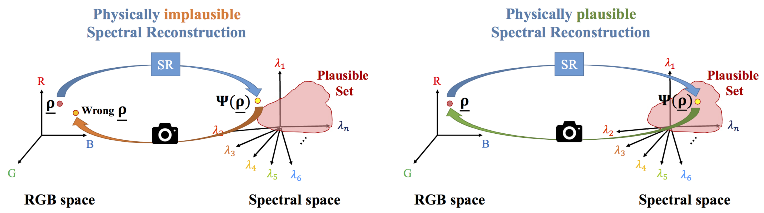
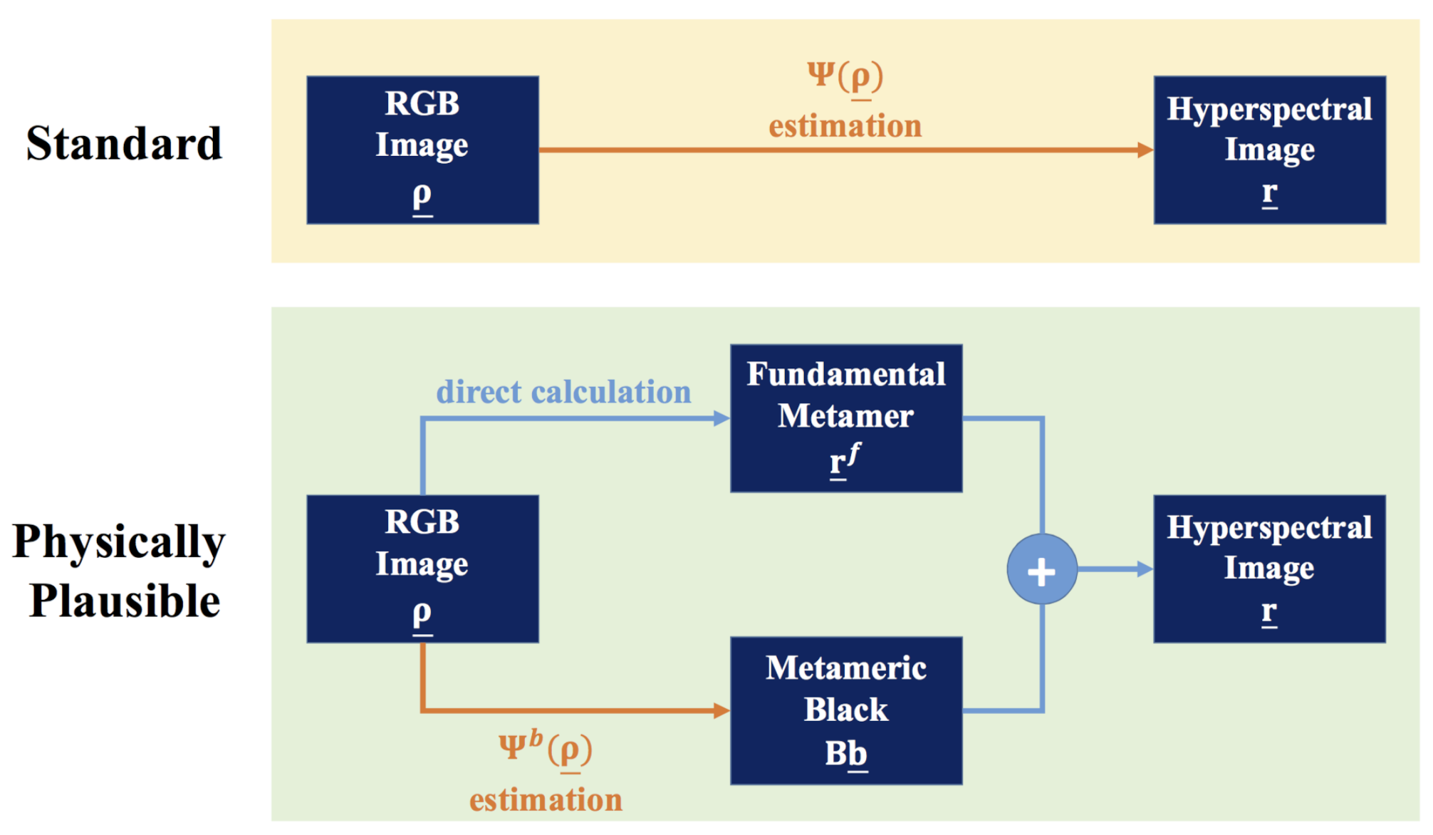
3. Physically Plausible Spectral Reconstruction
3.1. The Plausible Set
3.2. Estimating Physically Plausible Spectra from RGBs
3.2.1. Physically Plausible Regression-Based Models
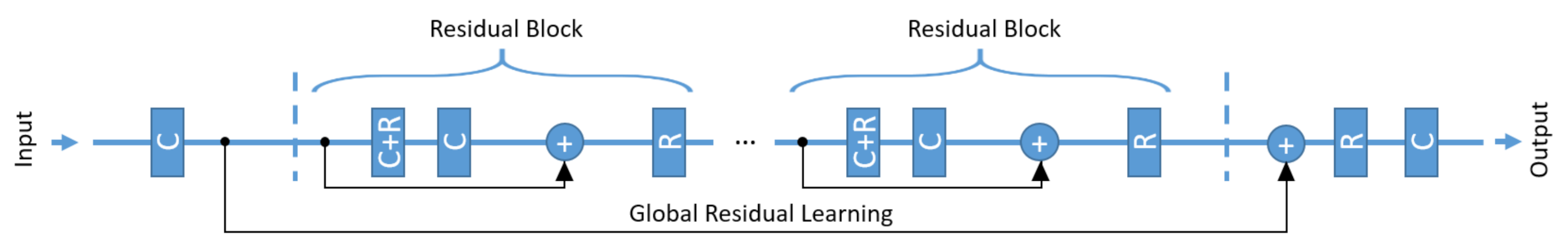
3.2.2. Physically Plausible Deep Neural Networks
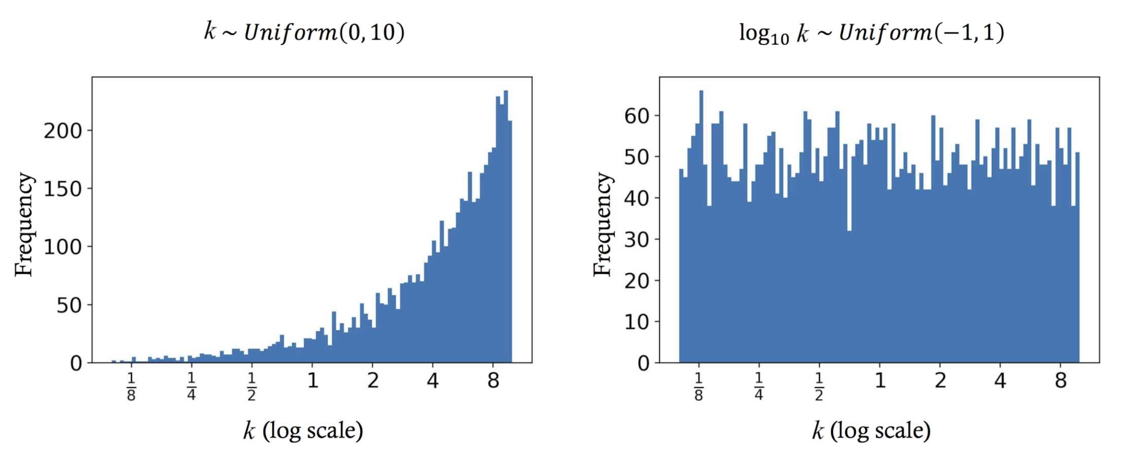
3.3. Intensity-Scaling Data Augmentation
4. Experiments
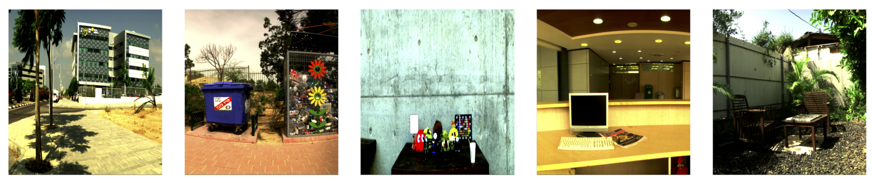
4.1. Image Dataset
4.2. Cross Validation
- Trial 1—Train set: , Validation set: C, Test set: D,
- Trial 2—Train set: , Validation set: D, Test set: C,
- Trial 3—Train set: , Validation set: A, Test set: B,
- Trial 4—Train set: , Validation set: B, Test set: A.
4.3. Evaluation Metrics
4.3.1. Spectral Difference
- Mean relative absolute error:where n is the number of spectral channels (in our case ), the division is element-wise and the L1 norm is calculated. Essentially, this MRAE metric measures the averaged percentage absolute deviation over all spectral channels. This metric is regarded as the standard metric to rank and evaluate SR algorithms in the recent benchmark [47,48].
- Goodness of fit coefficient:where the inner product of the normalized spectra is calculated. According to [56], acceptable reconstruction performance refers to GFC , GFC is regarded as very good performance and GFC means nearly exact reconstruction.
- Root mean square error:where n is the number of spectral channels. Note that RMSE is scale dependent, that is, the overall brightness level in which the compared spectra reside will reflect on the scale of RMSE. Thus, bear in mind that the images in the ICVL database [45] use 12-bit encoding (i.e., all values are bounded by [0, 4095]) when interpreting the presented results.
- Peak signal-to-noise ratio:where is the maximum possible value for 12-bit images. Similarly to RMSE, PSNR is scale dependent.
4.3.2. Color Difference
5. Results
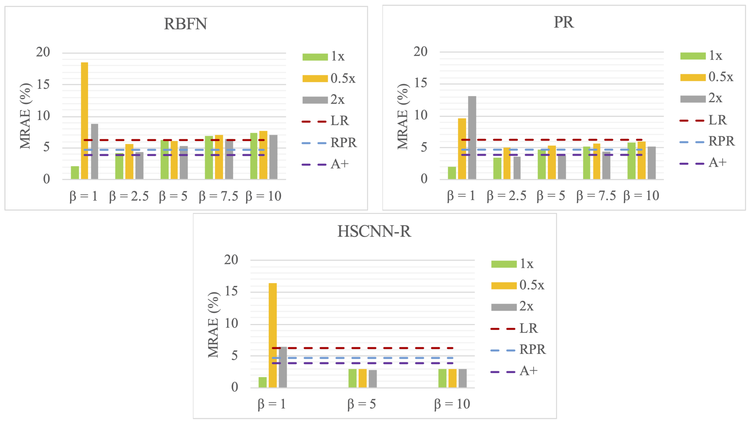
5.1. Effectiveness of Data Augmentation
5.2. Effectiveness of Physically Plausible Spectral Reconstruction
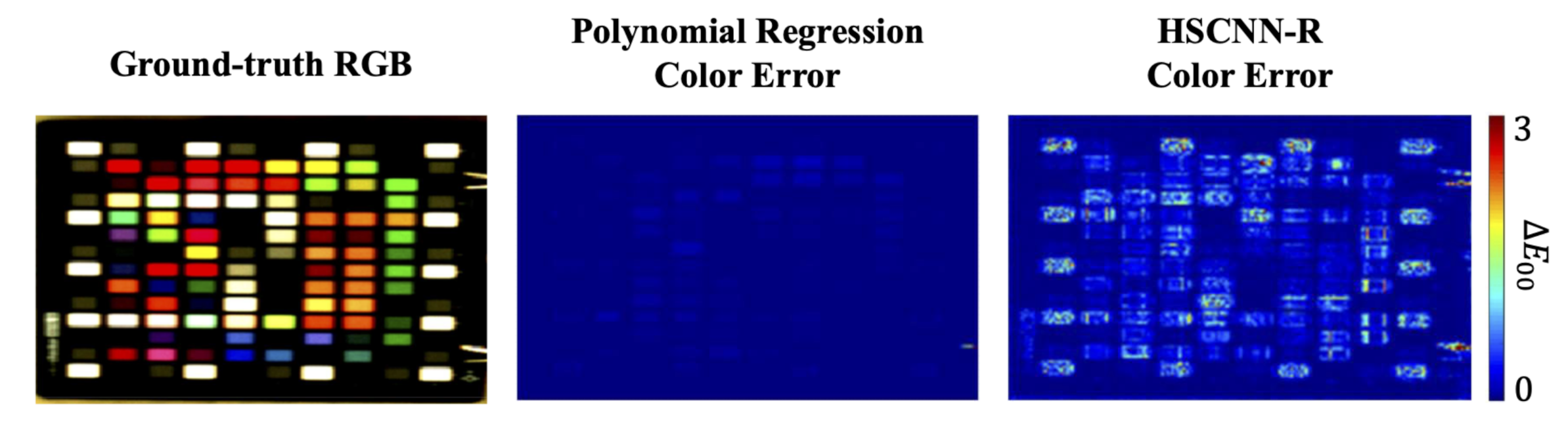
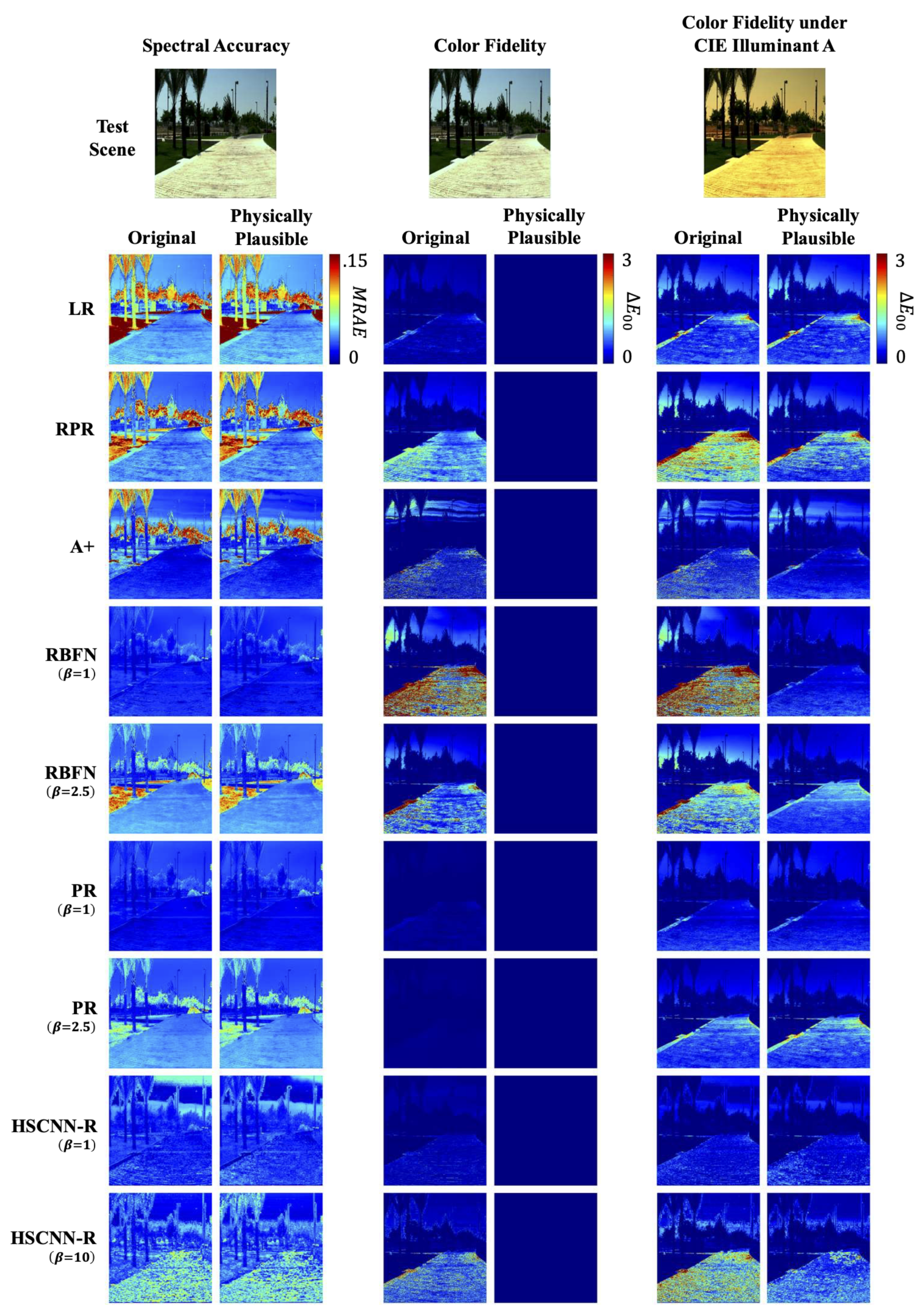
5.2.1. Color Fidelity and Spectral Accuracy
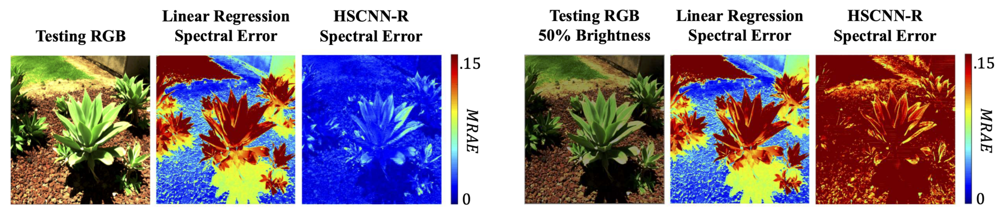
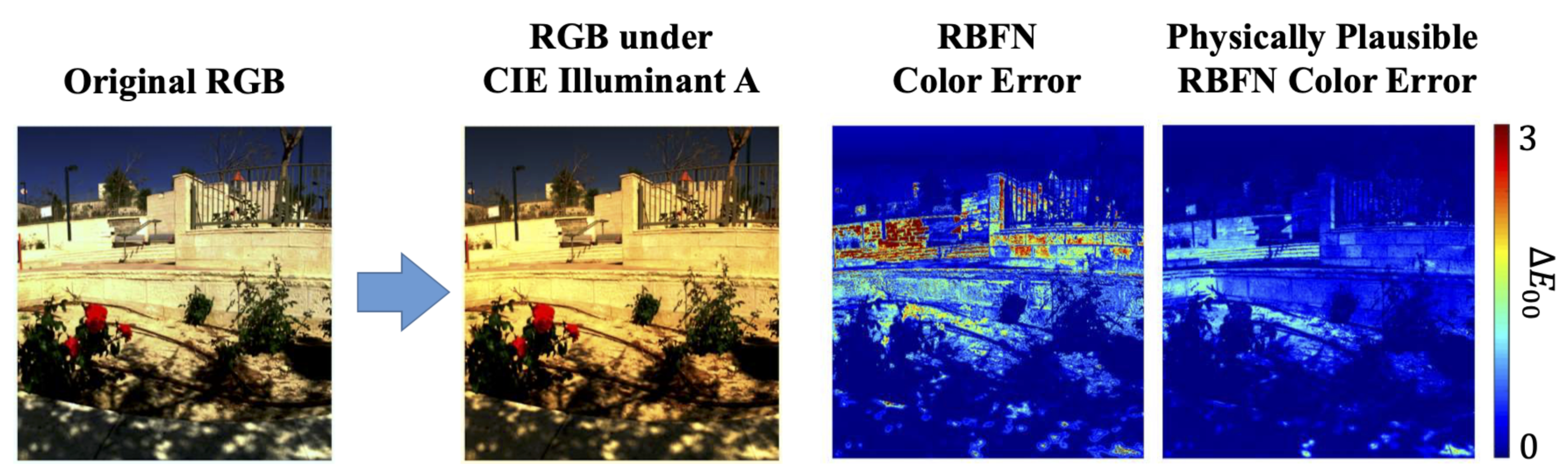
5.2.2. Color Fidelity under Different Viewing Conditions
6. Conclusions
Supplementary Materials
Author Contributions
Funding
Conflicts of Interest
References
- Veganzones, M.; Tochon, G.; Dalla-Mura, M.; Plaza, A.; Chanussot, J. Hyperspectral image segmentation using a new spectral unmixing-based binary partition tree representation. IEEE Trans. Image Process. 2014, 23, 3574–3589. [Google Scholar] [CrossRef] [PubMed]
- Chen, Y.; Zhao, X.; Jia, X. Spectral–spatial classification of hyperspectral data based on deep belief network. IEEE J. Sel. Top. Appl. Earth Obs. Remote Sens. 2015, 8, 2381–2392. [Google Scholar] [CrossRef]
- Ghamisi, P.; Dalla Mura, M.; Benediktsson, J. A survey on spectral—spatial classification techniques based on attribute profiles. IEEE Trans. Geosci. Remote. Sens. 2014, 53, 2335–2353. [Google Scholar] [CrossRef]
- Tao, C.; Pan, H.; Li, Y.; Zou, Z. Unsupervised spectral-spatial feature learning with stacked sparse autoencoder for hyperspectral imagery classification. IEEE Geosci. Remote Sens. Lett. 2015, 12, 2438–2442. [Google Scholar]
- Chen, C.; Li, W.; Su, H.; Liu, K. Spectral-spatial classification of hyperspectral image based on kernel extreme learning machine. Remote. Sens. 2014, 6, 5795–5814. [Google Scholar] [CrossRef]
- Jablonski, J.A.; Bihl, T.J.; Bauer, K.W. Principal component reconstruction error for hyperspectral anomaly detection. IEEE Geosci. Remote Sens. Lett. 2015, 12, 1725–1729. [Google Scholar] [CrossRef]
- Zhang, Y.; Mou, X.; Wang, G.; Yu, H. Tensor-based dictionary learning for spectral CT reconstruction. IEEE Trans. Med Imaging 2016, 36, 142–154. [Google Scholar] [CrossRef]
- Zhang, Y.; Xi, Y.; Yang, Q.; Cong, W.; Zhou, J.; Wang, G. Spectral CT reconstruction with image sparsity and spectral mean. IEEE Trans. Comput. Imaging 2016, 2, 510–523. [Google Scholar] [CrossRef]
- Deering, M. Multi-Spectral Color Correction. U.S. Patent 6,950,109, 27 September 2005. [Google Scholar]
- Abrardo, A.; Alparone, L.; Cappellini, I.; Prosperi, A. Color constancy from multispectral images. In Proceedings of the International Conference on Image Processing, Kobe, Japan, 24–28 October 1999; Volume 3, pp. 570–574. [Google Scholar]
- Cheung, V.; Westland, S.; Li, C.; Hardeberg, J.; Connah, D. Characterization of trichromatic color cameras by using a new multispectral imaging technique. J. Opt. Soc. Am. A 2005, 22, 1231–1240. [Google Scholar] [CrossRef]
- Lam, A.; Sato, I. Spectral modeling and relighting of reflective-fluorescent scenes. In Proceedings of the Conference on Computer Vision and Pattern Recognition, Portland, OR, USA, 23–28 June 2013; pp. 1452–1459. [Google Scholar]
- Xu, P.; Xu, H.; Diao, C.; Ye, Z. Self-training-based spectral image reconstruction for art paintings with multispectral imaging. Appl. Opt. 2017, 56, 8461–8470. [Google Scholar] [CrossRef]
- Gat, N. Imaging spectroscopy using tunable filters: A review. In Proceedings of the Wavelet Applications VII, International Society for Optics and Photonics, Orlando, FL, USA, 26 July 2000; Volume 4056, pp. 50–64. [Google Scholar]
- Green, R.O.; Eastwood, M.L.; Sarture, C.M.; Chrien, T.G.; Aronsson, M.; Chippendale, B.J.; Faust, J.A.; Pavri, B.E.; Chovit, C.J.; Solis, M.; et al. Imaging spectroscopy and the airborne visible/infrared imaging spectrometer (AVIRIS). Remote Sens. Environ. 1998, 65, 227–248. [Google Scholar] [CrossRef]
- Cao, X.; Du, H.; Tong, X.; Dai, Q.; Lin, S. A prism-mask system for multispectral video acquisition. IEEE Trans. Pattern Anal. Mach. Intell. 2011, 33, 2423–2435. [Google Scholar]
- Correa, C.V.; Arguello, H.; Arce, G.R. Snapshot colored compressive spectral imager. J. Opt. Soc. Am. A 2015, 32, 1754–1763. [Google Scholar] [CrossRef] [PubMed]
- Garcia, H.; Correa, C.V.; Arguello, H. Multi-resolution compressive spectral imaging reconstruction from single pixel measurements. IEEE Trans. Image Process. 2018, 27, 6174–6184. [Google Scholar] [CrossRef] [PubMed]
- Arguello, H.; Arce, G.R. Colored coded aperture design by concentration of measure in compressive spectral imaging. IEEE Trans. Image Process. 2014, 23, 1896–1908. [Google Scholar] [CrossRef]
- Galvis, L.; Lau, D.; Ma, X.; Arguello, H.; Arce, G.R. Coded aperture design in compressive spectral imaging based on side information. Appl. Opt. 2017, 56, 6332–6340. [Google Scholar] [CrossRef]
- Lin, X.; Liu, Y.; Wu, J.; Dai, Q. Spatial-spectral encoded compressive hyperspectral imaging. ACM Trans. Graph. 2014, 33, 233. [Google Scholar] [CrossRef]
- Rueda, H.; Arguello, H.; Arce, G.R. DMD-based implementation of patterned optical filter arrays for compressive spectral imaging. J. Opt. Soc. Am. A 2015, 32, 80–89. [Google Scholar] [CrossRef]
- Zhao, Y.; Guo, H.; Ma, Z.; Cao, X.; Yue, T.; Hu, X. Hyperspectral Imaging With Random Printed Mask. In Proceedings of the Conference on Computer Vision and Pattern Recognition, Long Beach, CA, USA, 15–20 June 2019; pp. 10149–10157. [Google Scholar]
- Shrestha, R.; Hardeberg, J.Y.; Khan, R. Spatial arrangement of color filter array for multispectral image acquisition. In Proceedings of the Sensors, Cameras, and Systems for Industrial, Scientific, and Consumer Applications XII, International Society for Optics and Photonics, San Francisco, CA, USA, 25–27 January 2011; p. 787503. [Google Scholar]
- Murakami, Y.; Yamaguchi, M.; Ohyama, N. Hybrid-resolution multispectral imaging using color filter array. Opt. Express 2012, 20, 7173–7183. [Google Scholar] [CrossRef]
- Mihoubi, S.; Losson, O.; Mathon, B.; Macaire, L. Multispectral demosaicing using intensity-based spectral correlation. In Proceedings of the International Conference on Image Processing Theory, Tools and Applications, Orleans, France, 10–13 November 2015; pp. 461–466. [Google Scholar]
- Brauers, J.; Schulte, N.; Aach, T. Multispectral filter-wheel cameras: Geometric distortion model and compensation algorithms. IEEE Trans. Image Process. 2008, 17, 2368–2380. [Google Scholar] [CrossRef] [PubMed]
- Wang, L.; Xiong, Z.; Gao, D.; Shi, G.; Zeng, W.; Wu, F. High-speed hyperspectral video acquisition with a dual-camera architecture. In Proceedings of the Conference on Computer Vision and Pattern Recognition, Boston, MA, USA, 7–12 June 2015; pp. 4942–4950. [Google Scholar]
- Park, J.I.; Lee, M.H.; Grossberg, M.D.; Nayar, S.K. Multispectral imaging using multiplexed illumination. In Proceedings of the International Conference on Computer Vision, Rio De Janeiro, Brazil, 14–21 October 2007; pp. 1–8. [Google Scholar]
- Hirai, K.; Tanimoto, T.; Yamamoto, K.; Horiuchi, T.; Tominaga, S. An LED-based spectral imaging system for surface reflectance and normal estimation. In Proceedings of the International Conference on Signal-Image Technology & Internet-Based Systems, Kyoto, Japan, 2–5 December 2013; pp. 441–447. [Google Scholar]
- Shrestha, R.; Hardeberg, J.Y.; Mansouri, A. One-shot multispectral color imaging with a stereo camera. In Proceedings of the Digital Photography VII, International Society for Optics and Photonics, San Francisco, CA, USA, 24–25 January 2011; p. 787609. [Google Scholar]
- Takatani, T.; Aoto, T.; Mukaigawa, Y. One-shot hyperspectral imaging using faced reflectors. In Proceedings of the Conference on Computer Vision and Pattern Recognition, Honolulu, HI, USA, 21–26 July 2017; pp. 4039–4047. [Google Scholar]
- Heikkinen, V.; Lenz, R.; Jetsu, T.; Parkkinen, J.; Hauta-Kasari, M.; Jääskeläinen, T. Evaluation and unification of some methods for estimating reflectance spectra from RGB images. J. Opt. Soc. Am. A 2008, 25, 2444–2458. [Google Scholar] [CrossRef]
- Connah, D.; Hardeberg, J. Spectral recovery using polynomial models. In Proceedings of the Color Imaging X: Processing, Hardcopy, and Applications, International Society for Optics and Photonics, San Jose, CA, USA, 17 January 2005; Volume 5667, pp. 65–75. [Google Scholar]
- Lin, Y.; Finlayson, G. Exposure Invariance in Spectral Reconstruction from RGB Images. In Proceedings of the Color and Imaging Conference, Society for Imaging Science and Technology, Paris, France, 21–25 October 2019; Volume 2019, pp. 284–289. [Google Scholar]
- Nguyen, R.; Prasad, D.; Brown, M. Training-based spectral reconstruction from a single RGB image. In Proceedings of the European Conference on Computer Vision, Zurich, Switzerland, 6–12 September 2014; pp. 186–201. [Google Scholar]
- Aeschbacher, J.; Wu, J.; Timofte, R. In defense of shallow learned spectral reconstruction from RGB images. In Proceedings of the International Conference on Computer Vision, Venice, Italy, 22–29 October 2017; pp. 471–479. [Google Scholar]
- Maloney, L.T.; Wandell, B.A. Color constancy: A method for recovering surface spectral reflectance. J. Opt. Soc. Am. A 1986, 3, 29–33. [Google Scholar] [CrossRef]
- Agahian, F.; Amirshahi, S.A.; Amirshahi, S.H. Reconstruction of reflectance spectra using weighted principal component analysis. Color Res. Appl. 2008, 33, 360–371. [Google Scholar] [CrossRef]
- Zhao, Y.; Berns, R.S. Image-based spectral reflectance reconstruction using the matrix R method. Color Res. Appl. 2007, 32, 343–351. [Google Scholar] [CrossRef]
- Brainard, D.H.; Freeman, W.T. Bayesian color constancy. J. Opt. Soc. Am. A 1997, 14, 1393–1411. [Google Scholar] [CrossRef]
- Morovic, P.; Finlayson, G.D. Metamer-set-based approach to estimating surface reflectance from camera RGB. J. Opt. Soc. Am. A 2006, 23, 1814–1822. [Google Scholar] [CrossRef]
- Bianco, S. Reflectance spectra recovery from tristimulus values by adaptive estimation with metameric shape correction. J. Opt. Soc. Am. A 2010, 27, 1868–1877. [Google Scholar] [CrossRef]
- Zuffi, S.; Santini, S.; Schettini, R. From color sensor space to feasible reflectance spectra. IEEE Trans. Signal Process. 2008, 56, 518–531. [Google Scholar] [CrossRef]
- Arad, B.; Ben-Shahar, O. Sparse recovery of hyperspectral signal from natural RGB images. In Proceedings of the European Conference on Computer Vision, Amsterdam, The Netherlands, 11–14 October 2016; pp. 19–34. [Google Scholar]
- Shi, Z.; Chen, C.; Xiong, Z.; Liu, D.; Wu, F. Hscnn+: Advanced cnn-based hyperspectral recovery from RGB images. In Proceedings of the Conference on Computer Vision and Pattern Recognition Workshops, Perth, Australia, 2–6 December 2018; pp. 939–947. [Google Scholar]
- Arad, B.; Ben-Shahar, O.; Timofte, R. NTIRE 2018 challenge on spectral reconstruction from RGB images. In Proceedings of the Conference on Computer Vision and Pattern Recognition Workshops, Salt Lake City, UT, USA, 18–22 June 2018; pp. 929–938. [Google Scholar]
- Arad, B.; Timofte, R.; Ben-Shahar, O.; Lin, Y.; Finlayson, G. NTIRE 2020 challenge on spectral reconstruction from an RGB image. In Proceedings of the Conference on Computer Vision and Pattern Recognition Workshops, Seattle, WA, USA, 14–19 June 2020. [Google Scholar]
- Arun, P.; Buddhiraju, K.; Porwal, A.; Chanussot, J. CNN based spectral super-resolution of remote sensing images. Signal Process. 2020, 169, 107394. [Google Scholar] [CrossRef]
- Li, J.; Wu, C.; Song, R.; Li, Y.; Liu, F. Adaptive weighted attention network with camera spectral sensitivity prior for spectral reconstruction from RGB images. In Proceedings of the Conference on Computer Vision and Pattern Recognition Workshops, Seattle, WA, USA, 14–19 June 2020; pp. 462–463. [Google Scholar]
- Joslyn Fubara, B.; Sedky, M.; Dyke, D. RGB to Spectral Reconstruction via Learned Basis Functions and Weights. In Proceedings of the Conference on Computer Vision and Pattern Recognition Workshops, Seattle, WA, USA, 14–19 June 2020; pp. 480–481. [Google Scholar]
- Chakrabarti, A.; Zickler, T. Statistics of real-world hyperspectral images. In Proceedings of the Conference on Computer Vision and Pattern Recognition, Colorado Springs, CO, USA, 20–25 June 2011; pp. 193–200. [Google Scholar]
- Zhao, Y.; Po, L.M.; Yan, Q.; Liu, W.; Lin, T. Hierarchical regression network for spectral reconstruction from RGB images. In Proceedings of the Conference on Computer Vision and Pattern Recognition Workshops, Seattle, WA, USA, 14–19 June 2020; pp. 422–423. [Google Scholar]
- Sharma, G.; Wu, W.; Dalal, E.N. The CIEDE2000 color-difference formula: Implementation notes, supplementary test data, and mathematical observations. Color Res. Appl. 2005, 30, 21–30. [Google Scholar] [CrossRef]
- Hardeberg, J.Y. On the spectral dimensionality of object colours. In Proceedings of the Conference on Colour in Graphics, Imaging, and Vision, Society for Imaging Science and Technology, Poitiers, France, 2–5 April 2002; Volume 2002, pp. 480–485. [Google Scholar]
- Romero, J.; Garcıa-Beltrán, A.; Hernández-Andrés, J. Linear bases for representation of natural and artificial illuminants. J. Opt. Soc. Am. A 1997, 14, 1007–1014. [Google Scholar] [CrossRef]
- Lee, T.W.; Wachtler, T.; Sejnowski, T.J. The spectral independent components of natural scenes. In Proceedings of the International Workshop on Biologically Motivated Computer Vision, Seoul, Korea, 15–17 May 2000; pp. 527–534. [Google Scholar]
- Marimont, D.H.; Wandell, B.A. Linear models of surface and illuminant spectra. J. Opt. Soc. Am. A 1992, 9, 1905–1913. [Google Scholar] [CrossRef]
- Parkkinen, J.P.; Hallikainen, J.; Jaaskelainen, T. Characteristic spectra of Munsell colors. J. Opt. Soc. Am. A 1989, 6, 318–322. [Google Scholar] [CrossRef]
- Strang, G. Introduction to Linear Algebra, 5th ed.; Wellesley-Cambridge Press: Wellesley, MA, USA, 2016; pp. 135–149; 219–232; 382–391. [Google Scholar]
- Finlayson, G.; Morovic, P. Metamer sets. J. Opt. Soc. Am. A 2005, 22, 810–819. [Google Scholar] [CrossRef]
- Bashkatov, A.; Genina, E.; Kochubey, V.; Tuchin, V. Optical properties of the subcutaneous adipose tissue in the spectral range 400–2500 nm. Opt. Spectrosc. 2005, 99, 836–842. [Google Scholar] [CrossRef]
- Pan, Z.; Healey, G.; Prasad, M.; Tromberg, B. Face recognition in hyperspectral images. IEEE Trans. Pattern Anal. Mach. Intell. 2003, 25, 1552–1560. [Google Scholar]
- Wandell, B.A. The synthesis and analysis of color images. IEEE Trans. Pattern Anal. Mach. Intell. 1987, 1, 2–13. [Google Scholar] [CrossRef] [PubMed]
- Aharon, M.; Elad, M.; Bruckstein, A. K-SVD: An algorithm for designing overcomplete dictionaries for sparse representation. IEEE Trans. Signal Process. 2006, 54, 4311–4322. [Google Scholar] [CrossRef]
- Tikhonov, A.; Goncharsky, A.; Stepanov, V.; Yagola, A. Numerical Methods for the Solution of Ill-Posed Problems; Springer Science & Business Media: Berlin/Heidelberg, Germany, 2013; Volume 328. [Google Scholar]
- Webb, G.I. Overfitting. In Encyclopedia of Machine Learning; Sammut, C., Webb, G.I., Eds.; Springer: Boston, MA, USA, 2010; p. 744. [Google Scholar] [CrossRef]
- He, K.; Zhang, X.; Ren, S.; Sun, J. Deep residual learning for image recognition. In Proceedings of the Conference on Computer Vision and Pattern Recognition, Las Vegas, NV, USA, 27–30 June 2016; pp. 770–778. [Google Scholar]
- Cheney, W.; Kincaid, D. Linear Algebra: Theory and Applications; Jones & Bartlett Learning: Sudbury, MA, USA, 2009; Volume 110, pp. 544–558. [Google Scholar]
- Cohen, J.B.; Kappauf, W.E. Metameric color stimuli, fundamental metamers, and Wyszecki’s metameric blacks. Am. J. Psychol. 1982, 95, 537–564. [Google Scholar] [CrossRef]
- Commission Internationale de l’Eclairage. CIE Proceedings (1964) Vienna Session, Committee Report E-1.4; Commission Internationale de l’Eclairage: Vienna, Austria, 1964. [Google Scholar]
- Commission Internationale de l’Eclairage. Commission Internationale de L’eclairage Proceedings (1931); Cambridge University: Cambridge, UK, 1932. [Google Scholar]
- Robertson, A.R. The CIE 1976 color-difference formulae. Color Res. Appl. 1977, 2, 7–11. [Google Scholar] [CrossRef]
- Süsstrunk, S.; Buckley, R.; Swen, S. Standard RGB color spaces. In Proceedings of the Color and Imaging Conference, Society for Imaging Science and Technology, Scottsdale, AZ, USA, 16–19 November 1999; pp. 127–134. [Google Scholar]


| Exposure-Invariant Models | Non-Exposure-Invariant Models |
|---|---|
| Linear Regression (LR) [33] | Radial Basis Function Network (RBFN) [36] |
| Root-Polynomial Regression (RPR) [35] | Polynomial Regression (PR) [34] |
| A+ Sparse Coding (A+) [37] | HSCNN-R Deep Neural Network (HSCNN-R) [46] |
| Mean MRAE (%) (Spectral Error) | |||||||||||||||
| Baseline Performance: LR = 6.24, RPR = 4.69, A+ = 3.87 | |||||||||||||||
| 1x | 0.5x | 2x | 1x | 0.5x | 2x | 1x | 0.5x | 2x | 1x | 0.5x | 2x | 1x | 0.5x | 2x | |
| RBFN | 2.06 | 18.58 | 8.74 | 4.20 | 5.67 | 4.33 | 6.19 | 6.02 | 5.30 | 6.82 | 7.05 | 6.40 | 7.37 | 7.75 | 6.98 |
| PR | 1.95 | 9.60 | 13.04 | 3.50 | 5.01 | 3.57 | 4.72 | 5.40 | 3.80 | 5.25 | 5.72 | 4.45 | 5.74 | 6.03 | 5.13 |
| HSCNN-R | 1.73 | 16.41 | 6.39 | - | - | - | 2.91 | 2.92 | 2.81 | - | - | - | 2.96 | 2.96 | 2.95 |
| Mean GFC (Spectral Error) | |||||||||||||||
| Baseline Performance: LR = 0.9966, RPR = 0.9979, A+ = 0.9983 | |||||||||||||||
| 1x | 0.5x | 2x | 1x | 0.5x | 2x | 1x | 0.5x | 2x | 1x | 0.5x | 2x | 1x | 0.5x | 2x | |
| RBFN | 0.9994 | 0.9802 | 0.9959 | 0.9986 | 0.9981 | 0.9983 | 0.9977 | 0.9979 | 0.9981 | 0.9974 | 0.9971 | 0.9977 | 0.9973 | 0.9968 | 0.9976 |
| PR | 0.9994 | 0.9949 | 0.9900 | 0.9989 | 0.9984 | 0.9986 | 0.9984 | 0.9981 | 0.9987 | 0.9981 | 0.9979 | 0.9985 | 0.9979 | 0.9977 | 0.9982 |
| HSCNN-R | 0.9995 | 0.9889 | 0.9972 | - | - | - | 0.9992 | 0.9991 | 0.9992 | - | - | - | 0.9991 | 0.9991 | 0.9991 |
| Mean(Color Error) | |||||||||||||||
| Baseline Performance: LR = 0.05, RPR = 0.14, A+ = 0.06 | |||||||||||||||
| 1x | 0.5x | 2x | 1x | 0.5x | 2x | 1x | 0.5x | 2x | 1x | 0.5x | 2x | 1x | 0.5x | 2x | |
| RBFN | 0.32 | 0.68 | 1.97 | 0.15 | 0.17 | 0.37 | 0.51 | 0.61 | 0.76 | 0.81 | 1.03 | 1.00 | 0.95 | 1.24 | 1.20 |
| PR | 0.01 | 0.02 | 0.15 | 0.01 | 0.03 | 0.01 | 0.05 | 0.06 | 0.04 | 0.06 | 0.09 | 0.04 | 0.09 | 0.11 | 0.05 |
| HSCNN-R | 0.10 | 0.36 | 0.16 | - | - | - | 0.17 | 0.18 | 0.18 | - | - | - | 0.15 | 0.15 | 0.15 |
| (Color Error) | MRAE (%) (Spectral Error) | GFC (Spectral Error) | ||||||||||
| Original | Physically Plausible | Original | Physically Plausible | Original | Physically Plausible | |||||||
| Mean | 99.9 pt | Mean | 99.9 pt | Mean | 99.9 pt | Mean | 99.9 pt | Mean | 99.9 pt | Mean | 99.9 pt | |
| LR | 0.05 | 0.79 | 0.00 | 0.00 | 6.24 | 22.45 | 6.23 | 22.53 | 0.9966 | 0.9770 | 0.9966 | 0.9767 |
| RPR | 0.14 | 1.48 | 0.00 | 0.00 | 4.69 | 24.06 | 4.60 | 24.86 | 0.9979 | 0.9712 | 0.9979 | 0.9640 |
| A+ | 0.06 | 2.47 | 0.00 | 0.00 | 3.87 | 21.06 | 3.83 | 20.65 | 0.9983 | 0.9770 | 0.9983 | 0.9770 |
| RBFN | 0.32 | 9.24 | 0.00 | 0.00 | 2.06 | 14.44 | 1.96 | 13.09 | 0.9994 | 0.9852 | 0.9994 | 0.9854 |
| RBFN | 0.15 | 3.36 | 0.00 | 0.00 | 4.20 | 17.25 | 4.15 | 17.00 | 0.9986 | 0.9832 | 0.9986 | 0.9834 |
| PR | 0.01 | 0.18 | 0.00 | 0.00 | 1.95 | 12.84 | 1.94 | 12.81 | 0.9994 | 0.9841 | 0.9994 | 0.9843 |
| PR | 0.01 | 0.07 | 0.00 | 0.00 | 3.50 | 17.95 | 3.46 | 18.38 | 0.9989 | 0.9814 | 0.9989 | 0.9802 |
| HSCNN-R | 0.10 | 2.06 | 0.00 | 0.00 | 1.73 | 12.10 | 1.76 | 12.68 | 0.9995 | 0.9864 | 0.9995 | 0.9842 |
| HSCNN-R | 0.15 | 2.46 | 0.00 | 0.00 | 2.96 | 16.14 | 2.93 | 21.09 | 0.9991 | 0.9841 | 0.9991 | 0.9686 |
| RMSE (Spectral Error) | PSNR (dB) (Spectral Error) | |||||||||||
| Original | Physically Plausible | Original | Physically Plausible | |||||||||
| Mean | 99.9 pt | Mean | 99.9 pt | Mean | 99.9 pt | Mean | 99.9 pt | |||||
| LR | 33.26 | 153.49 | 33.23 | 153.35 | 43.34 | 30.24 | 43.36 | 30.33 | ||||
| RPR | 27.80 | 167.17 | 27.49 | 172.33 | 45.49 | 29.93 | 45.71 | 29.84 | ||||
| A+ | 23.97 | 161.69 | 24.36 | 165.61 | 48.23 | 29.79 | 48.21 | 29.65 | ||||
| RBFN | 18.30 | 152.57 | 17.50 | 138.23 | 50.63 | 31.04 | 50.98 | 31.62 | ||||
| RBFN | 27.70 | 142.46 | 27.24 | 139.51 | 45.54 | 30.84 | 45.67 | 31.06 | ||||
| PR | 17.05 | 142.31 | 17.06 | 142.55 | 50.86 | 31.72 | 50.86 | 31.71 | ||||
| PR | 23.88 | 143.93 | 23.75 | 146.78 | 47.03 | 31.07 | 47.10 | 30.96 | ||||
| HSCNN-R | 16.33 | 139.58 | 16.34 | 137.24 | 52.34 | 31.58 | 52.08 | 31.70 | ||||
| HSCNN-R | 23.56 | 167.82 | 22.67 | 165.65 | 49.07 | 29.47 | 49.38 | 29.55 | ||||
| Mean MRAE (%) | Mean GFC | Mean | |||||||
|---|---|---|---|---|---|---|---|---|---|
| (Spectral Error) | (Spectral Error) | (Color Error) | |||||||
| Physically Plausible | Physically Plausible | Physically Plausible | |||||||
| 1x | 0.5x | 2x | 1x | 0.5x | 2x | 1x | 0.5x | 2x | |
| LR | 6.23 | 6.23 | 6.23 | 0.9966 | 0.9966 | 0.9966 | 0.00 | 0.00 | 0.00 |
| RPR | 4.60 | 4.60 | 4.60 | 0.9979 | 0.9979 | 0.9979 | 0.00 | 0.00 | 0.00 |
| A+ | 3.83 | 3.83 | 3.83 | 0.9983 | 0.9983 | 0.9983 | 0.00 | 0.00 | 0.00 |
| RBFN | 1.96 | 17.6 | 7.63 | 0.9994 | 0.9773 | 0.9958 | 0.00 | 0.00 | 0.00 |
| RBFN | 4.15 | 5.47 | 4.19 | 0.9986 | 0.9982 | 0.9983 | 0.00 | 0.00 | 0.00 |
| PR | 1.94 | 9.72 | 13.07 | 0.9994 | 0.9948 | 0.9899 | 0.00 | 0.00 | 0.00 |
| PR | 3.46 | 4.93 | 3.55 | 0.9989 | 0.9984 | 0.9986 | 0.00 | 0.00 | 0.00 |
| HSCNN-R | 1.76 | 15.33 | 6.39 | 0.9995 | 0.9844 | 0.9972 | 0.00 | 0.00 | 0.00 |
| HSCNN-R | 2.93 | 3.00 | 2.88 | 0.9991 | 0.9991 | 0.9991 | 0.00 | 0.00 | 0.00 |
| (Color Error) | ||||||||||||
|---|---|---|---|---|---|---|---|---|---|---|---|---|
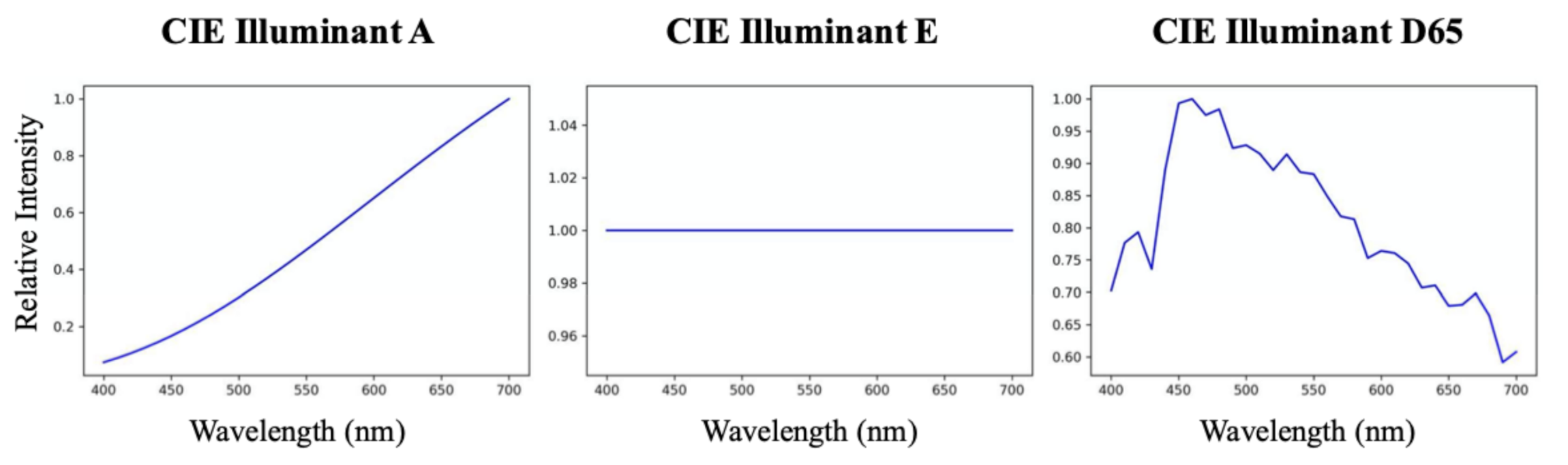
| CIE Illuminant A | CIE Illuminant E | CIE Illuminant D65 | ||||||||||
| Original | Physically Plausible | Original | Physically Plausible | Original | Physically Plausible | |||||||
| Mean | 99.9 pt | Mean | 99.9 pt | Mean | 99.9 pt | Mean | 99.9 pt | Mean | 99.9 pt | Mean | 99.9 pt | |
| LR | 0.38 | 3.89 | 0.38 | 4.00 | 0.57 | 6.58 | 0.56 | 6.33 | 0.49 | 6.05 | 0.47 | 5.67 |
| RPR | 0.32 | 4.89 | 0.29 | 4.36 | 0.51 | 6.49 | 0.46 | 6.26 | 0.44 | 5.83 | 0.39 | 5.66 |
| A+ | 0.27 | 4.90 | 0.24 | 4.53 | 0.40 | 6.72 | 0.38 | 6.02 | 0.34 | 6.33 | 0.31 | 5.51 |
| RBFN | 0.37 | 10.22 | 0.16 | 3.66 | 0.39 | 10.67 | 0.14 | 3.24 | 0.38 | 10.74 | 0.13 | 3.18 |
| RBFN | 0.41 | 5.80 | 0.35 | 3.97 | 0.58 | 7.28 | 0.54 | 5.69 | 0.49 | 6.79 | 0.45 | 5.07 |
| PR | 0.17 | 3.51 | 0.17 | 3.48 | 0.14 | 2.89 | 0.14 | 2.88 | 0.14 | 2.88 | 0.14 | 2.86 |
| PR | 0.26 | 3.77 | 0.25 | 3.74 | 0.46 | 5.36 | 0.45 | 5.30 | 0.38 | 4.79 | 0.37 | 4.73 |
| HSCNN-R | 0.18 | 4.12 | 0.15 | 3.75 | 0.18 | 3.91 | 0.12 | 2.92 | 0.18 | 4.06 | 0.12 | 2.95 |
| HSCNN-R | 0.31 | 5.41 | 0.26 | 4.95 | 0.53 | 7.67 | 0.43 | 7.12 | 0.44 | 7.03 | 0.35 | 6.29 |
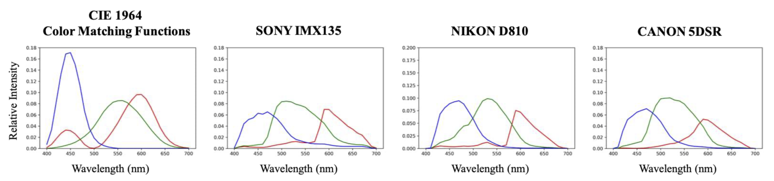
| (Color Error) | ||||||||||||
| SONY IMX135 | NIKON D810 | CANON 5DSR | ||||||||||
| Original | Physically Plausible | Original | Physically Plausible | Original | Physically Plausible | |||||||
| Mean | 99.9 pt | Mean | 99.9 pt | Mean | 99.9 pt | Mean | 99.9 pt | Mean | 99.9 pt | Mean | 99.9 pt | |
| LR | 0.33 | 3.39 | 0.33 | 3.36 | 0.63 | 5.90 | 0.63 | 5.83 | 0.41 | 3.95 | 0.41 | 3.89 |
| RPR | 0.28 | 3.93 | 0.26 | 3.76 | 0.54 | 6.74 | 0.53 | 6.72 | 0.38 | 4.75 | 0.35 | 4.52 |
| A+ | 0.27 | 4.93 | 0.24 | 4.37 | 0.49 | 8.33 | 0.45 | 7.86 | 0.34 | 5.88 | 0.30 | 5.29 |
| RBFN | 0.43 | 10.75 | 0.23 | 4.75 | 0.56 | 13.01 | 0.39 | 8.12 | 0.47 | 11.55 | 0.26 | 5.46 |
| RBFN | 0.36 | 4.92 | 0.30 | 3.33 | 0.71 | 6.48 | 0.66 | 5.26 | 0.47 | 5.22 | 0.40 | 3.50 |
| PR | 0.23 | 4.34 | 0.23 | 4.33 | 0.42 | 8.17 | 0.43 | 8.15 | 0.27 | 5.38 | 0.27 | 5.37 |
| PR | 0.24 | 3.52 | 0.23 | 3.53 | 0.51 | 6.11 | 0.50 | 6.16 | 0.33 | 3.94 | 0.32 | 3.97 |
| HSCNN-R | 0.26 | 5.26 | 0.24 | 4.99 | 0.42 | 8.70 | 0.40 | 8.60 | 0.29 | 5.97 | 0.27 | 5.71 |
| HSCNN-R | 0.35 | 5.75 | 0.28 | 5.10 | 0.62 | 9.36 | 0.56 | 9.06 | 0.43 | 6.40 | 0.36 | 5.97 |
Publisher’s Note: MDPI stays neutral with regard to jurisdictional claims in published maps and institutional affiliations. |
© 2020 by the authors. Licensee MDPI, Basel, Switzerland. This article is an open access article distributed under the terms and conditions of the Creative Commons Attribution (CC BY) license (http://creativecommons.org/licenses/by/4.0/).
Share and Cite
Lin, Y.-T.; Finlayson, G.D. Physically Plausible Spectral Reconstruction. Sensors 2020, 20, 6399. https://doi.org/10.3390/s20216399
Lin Y-T, Finlayson GD. Physically Plausible Spectral Reconstruction. Sensors. 2020; 20(21):6399. https://doi.org/10.3390/s20216399
Chicago/Turabian StyleLin, Yi-Tun, and Graham D. Finlayson. 2020. "Physically Plausible Spectral Reconstruction" Sensors 20, no. 21: 6399. https://doi.org/10.3390/s20216399
APA StyleLin, Y.-T., & Finlayson, G. D. (2020). Physically Plausible Spectral Reconstruction. Sensors, 20(21), 6399. https://doi.org/10.3390/s20216399