LiDAR-Camera Calibration Using Line Correspondences


Abstract
:1. Introduction
2. Related Work
3. Method
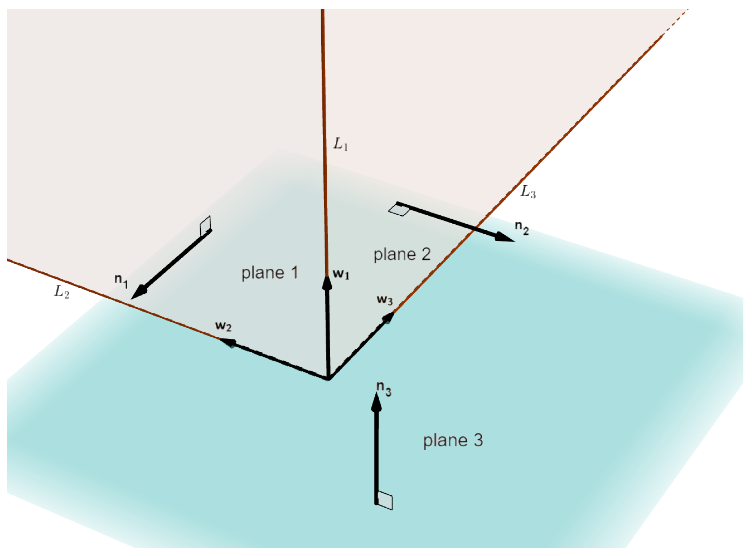
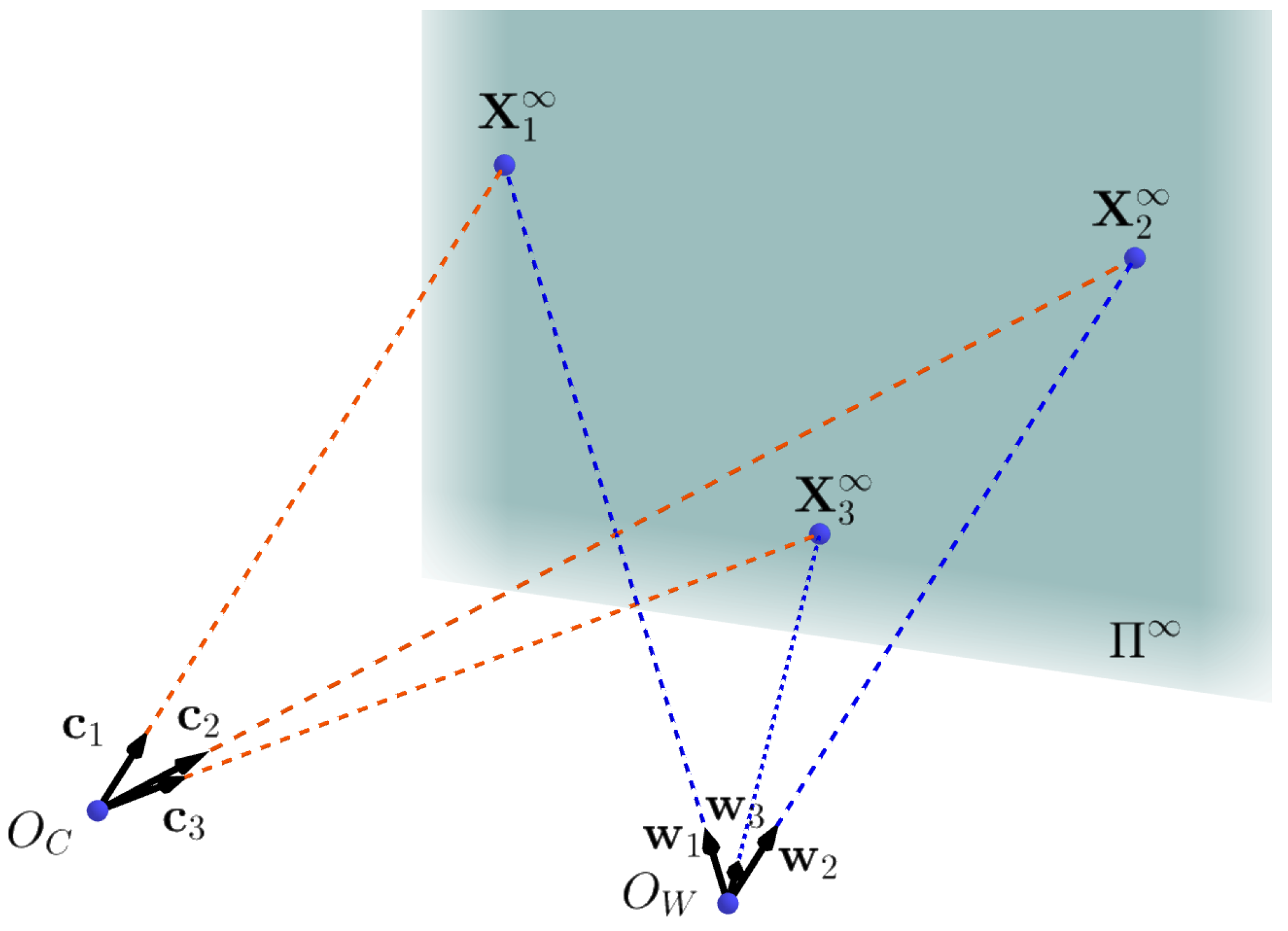
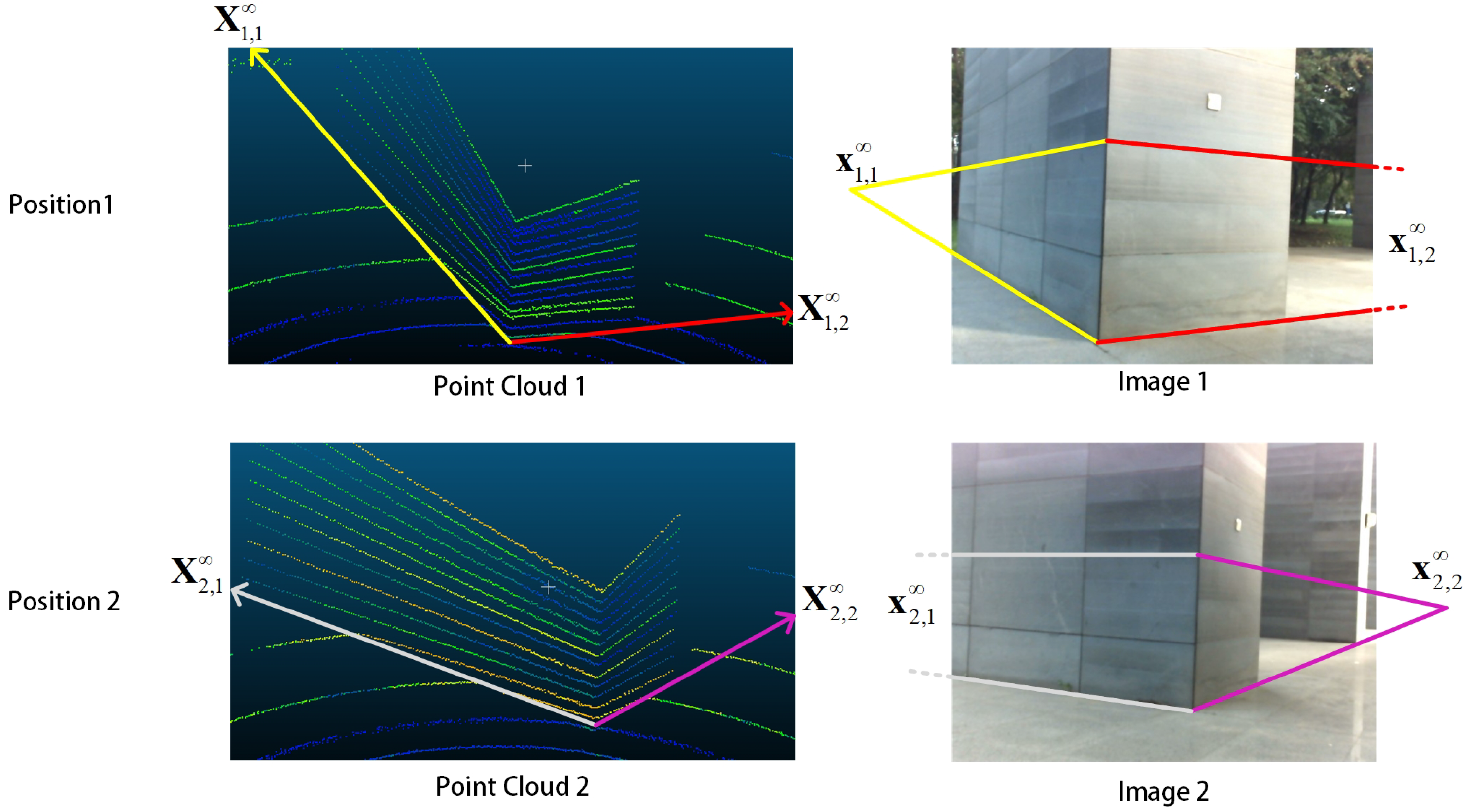
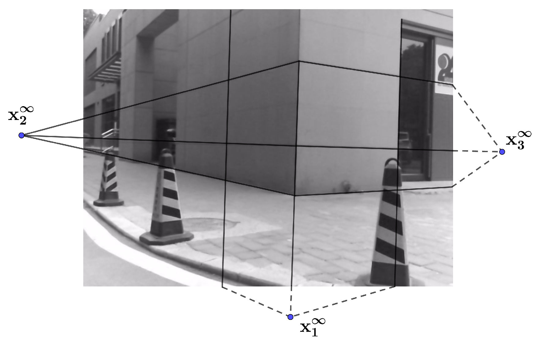
3.1. Solve Rotation Matrix with Infinity Point Pairs
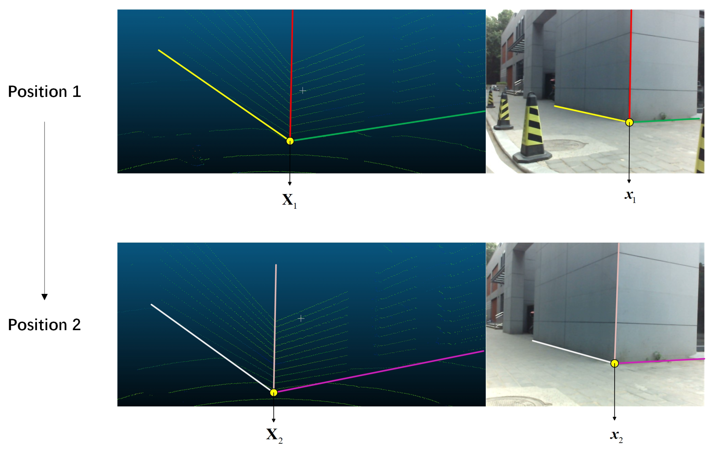
3.2. Solve Translation Vector
3.3. Optimization
| Algorithm 1: |
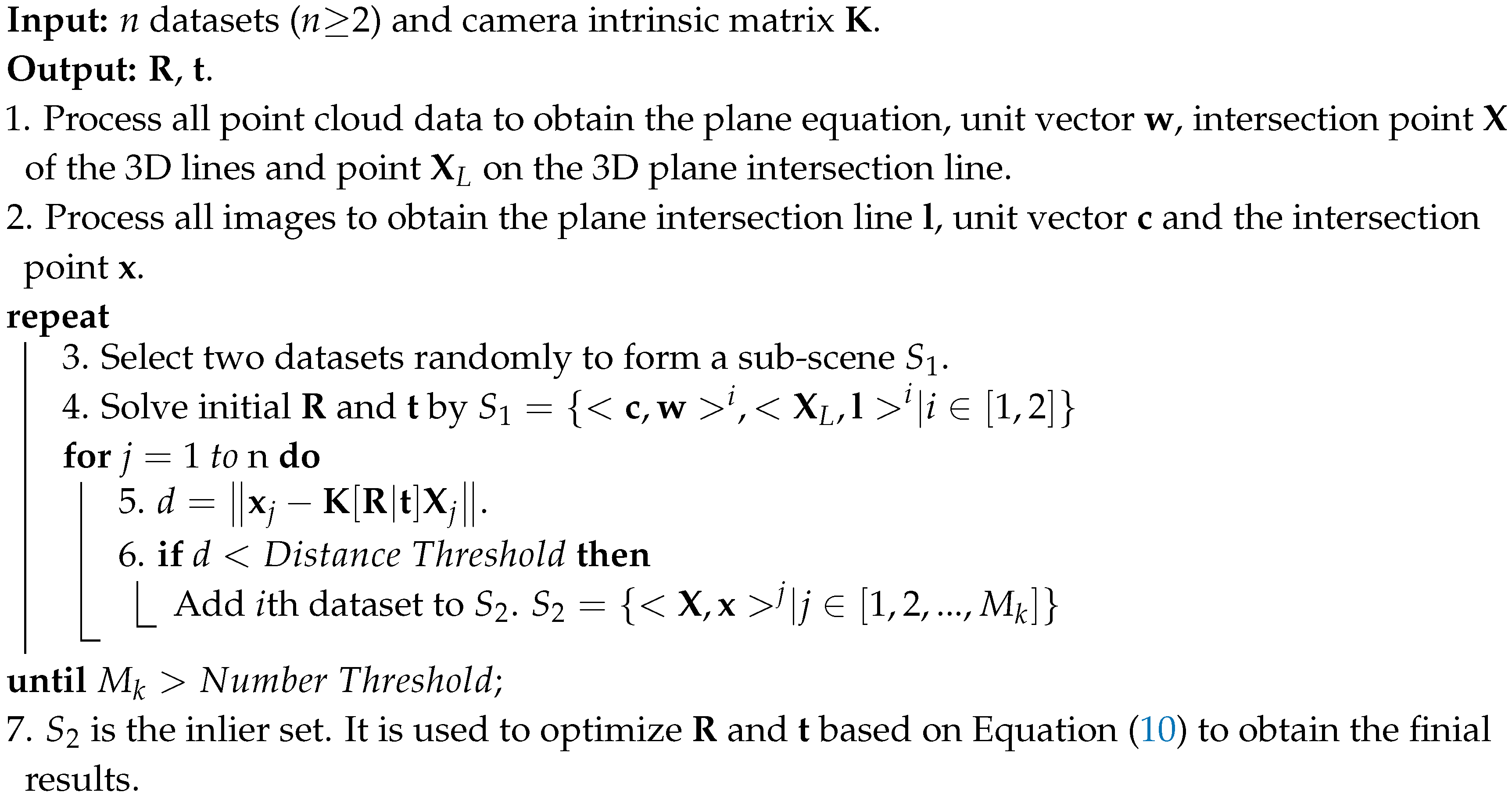 |
4. Experiments
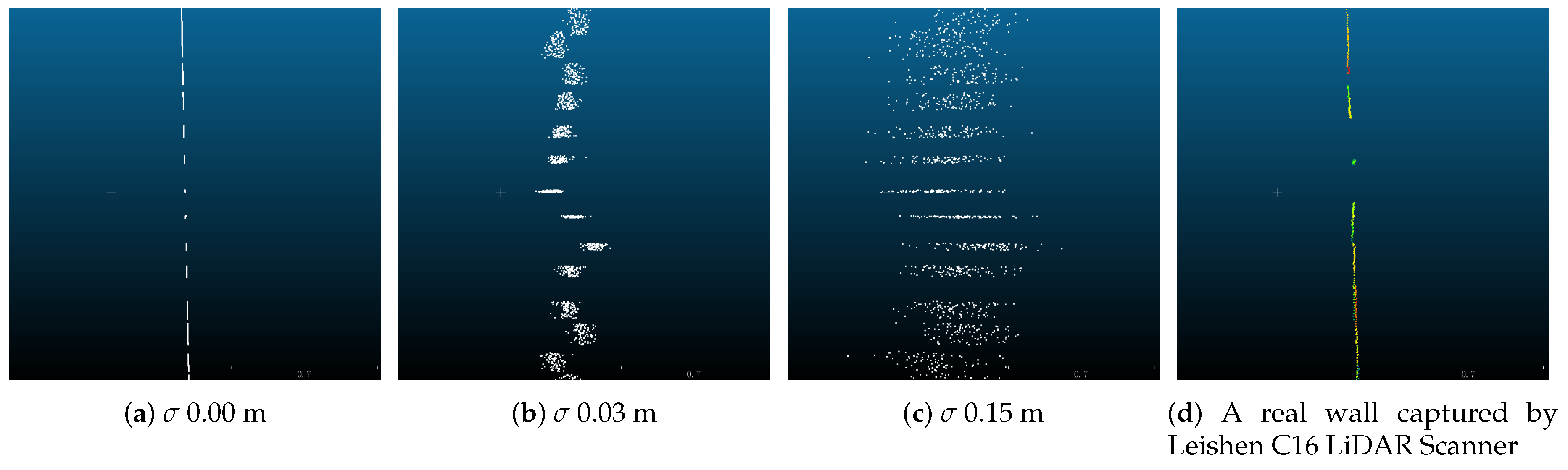
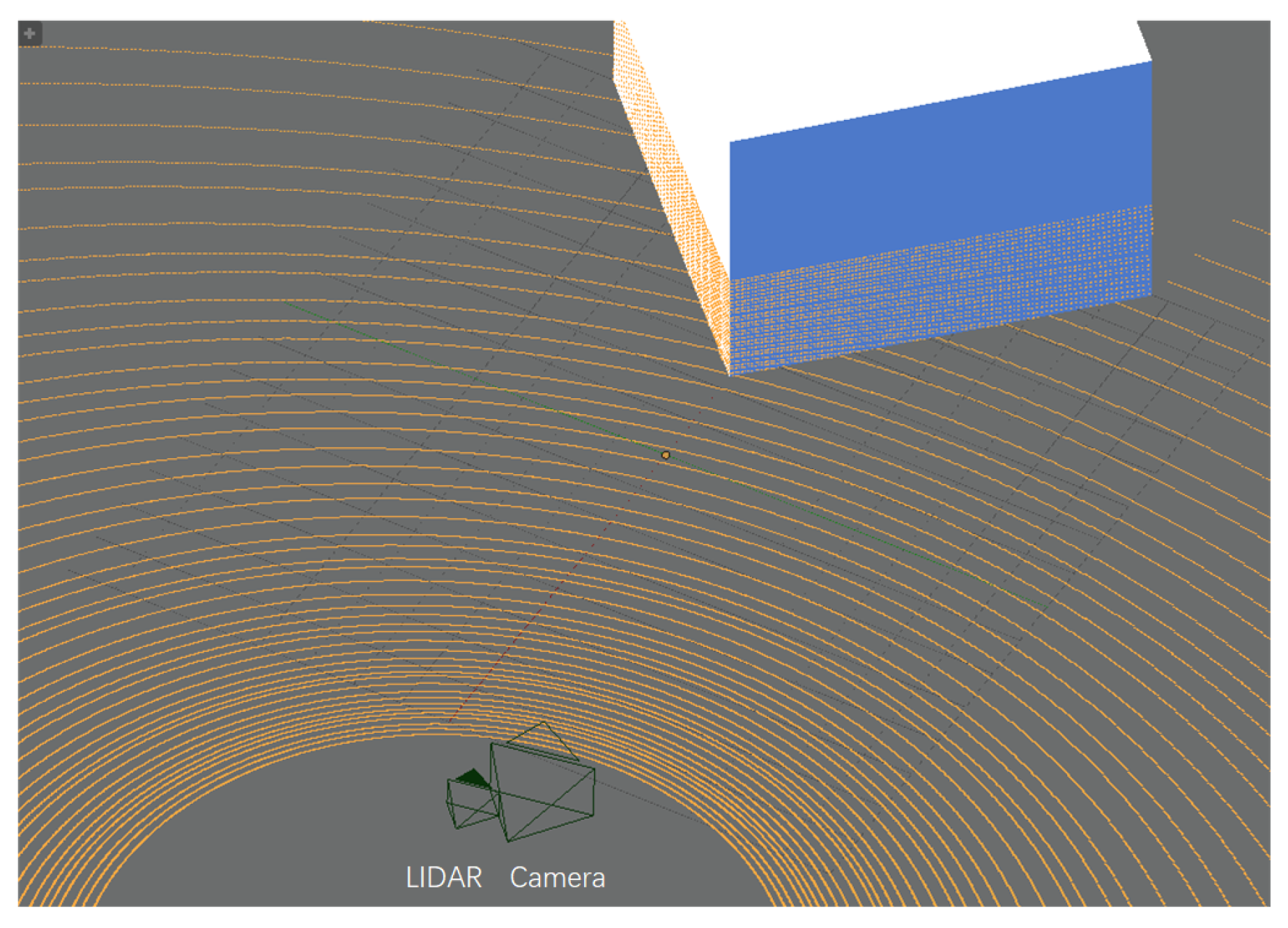
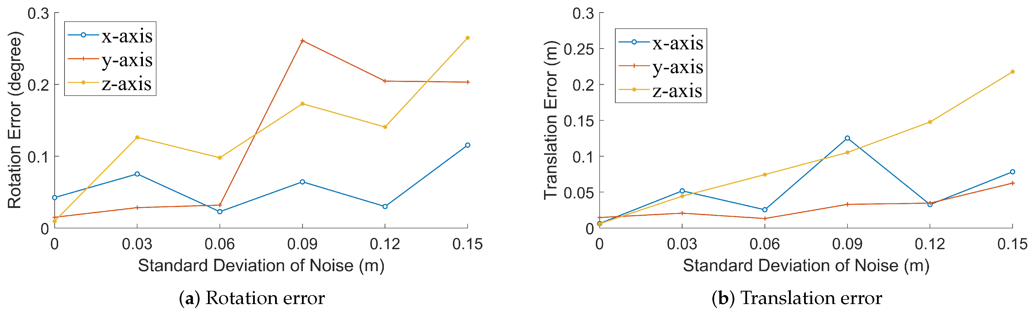
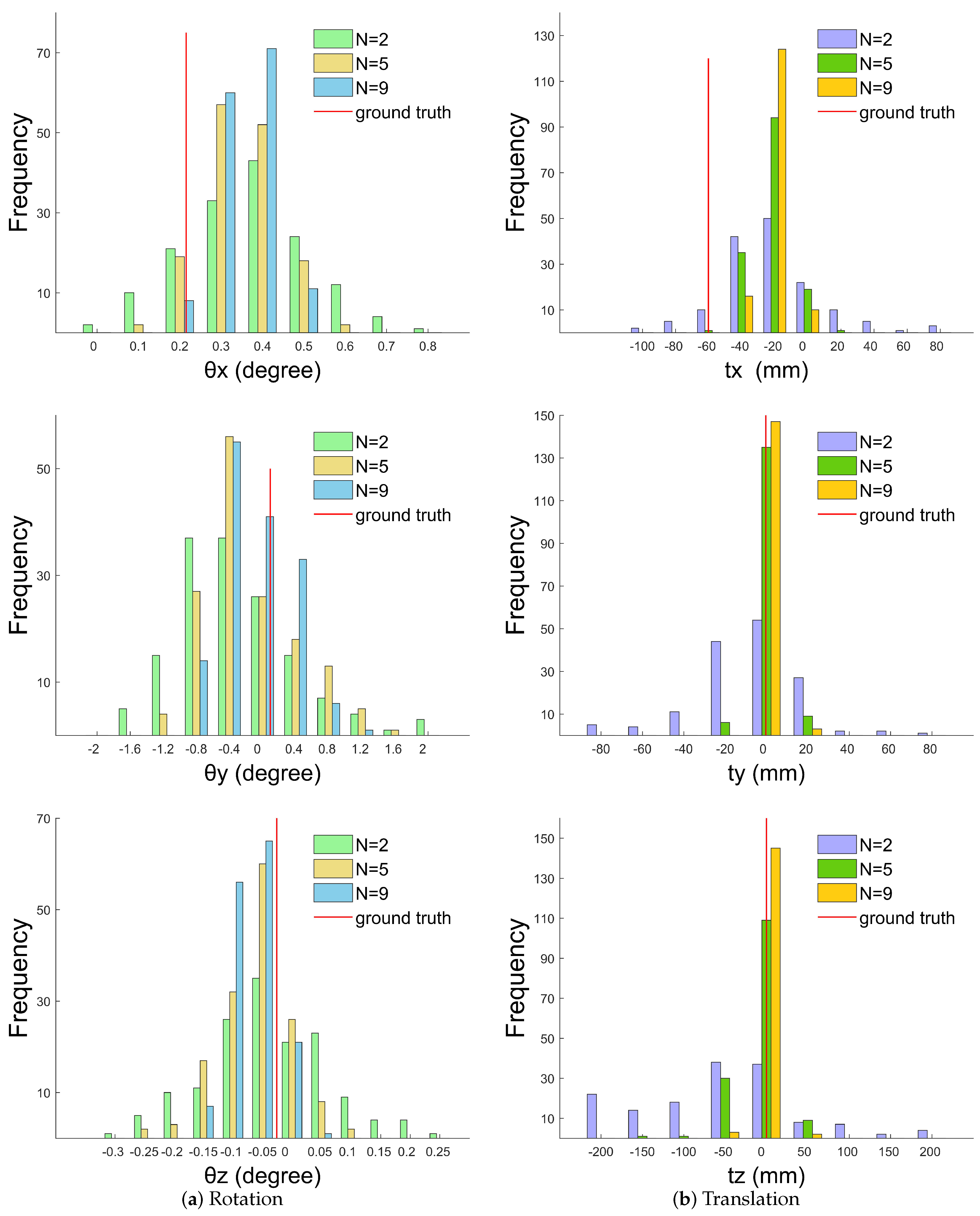
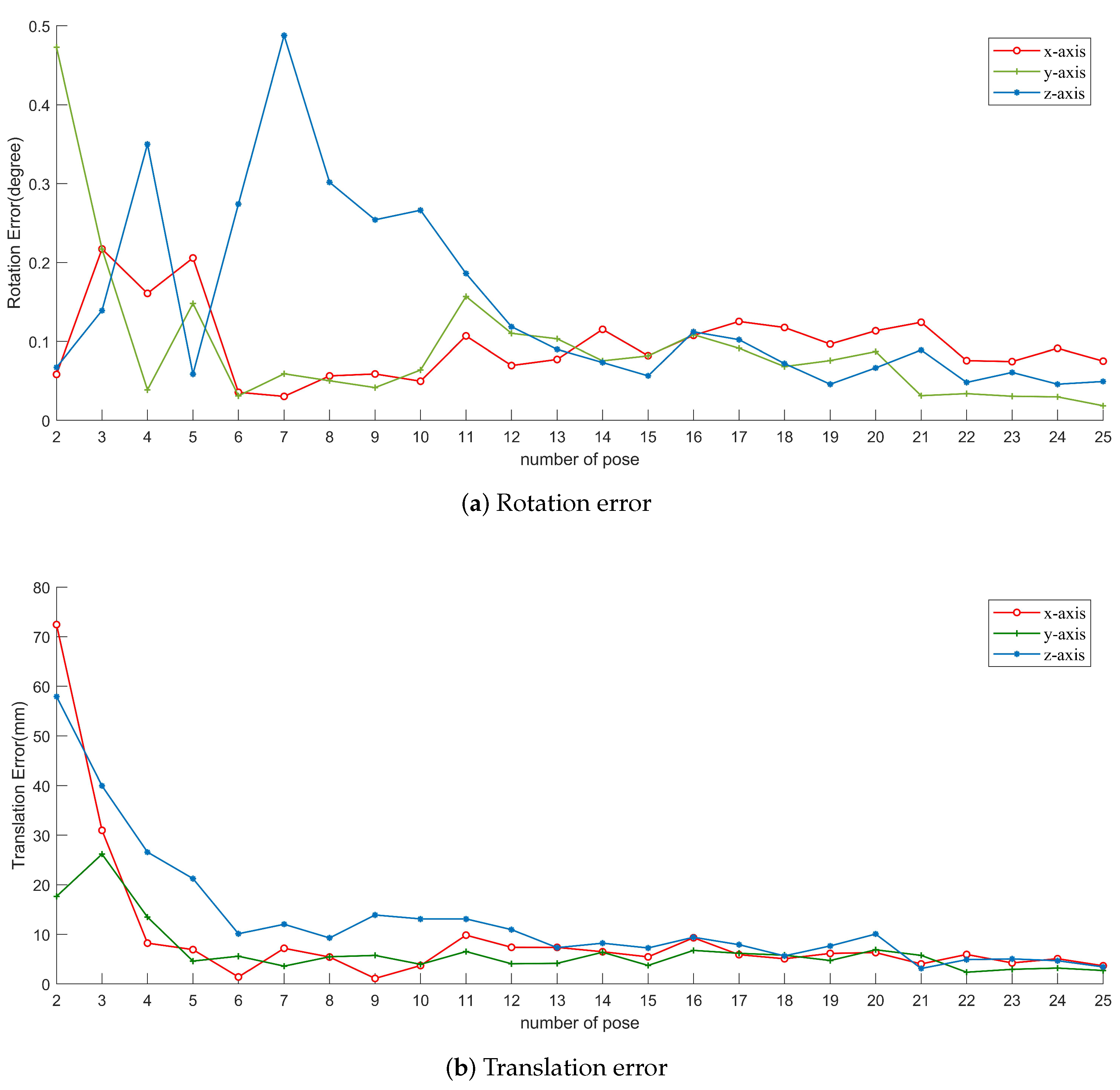
4.1. Simulated Data
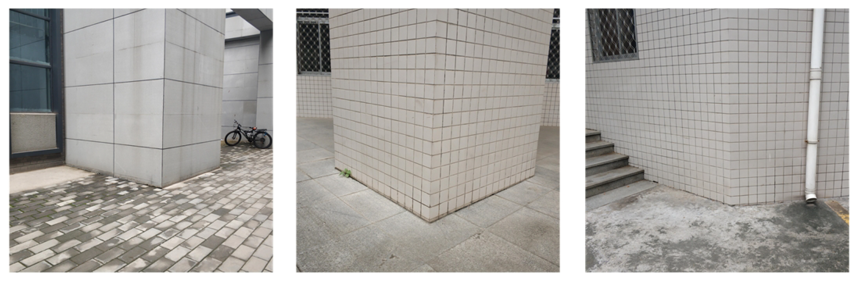
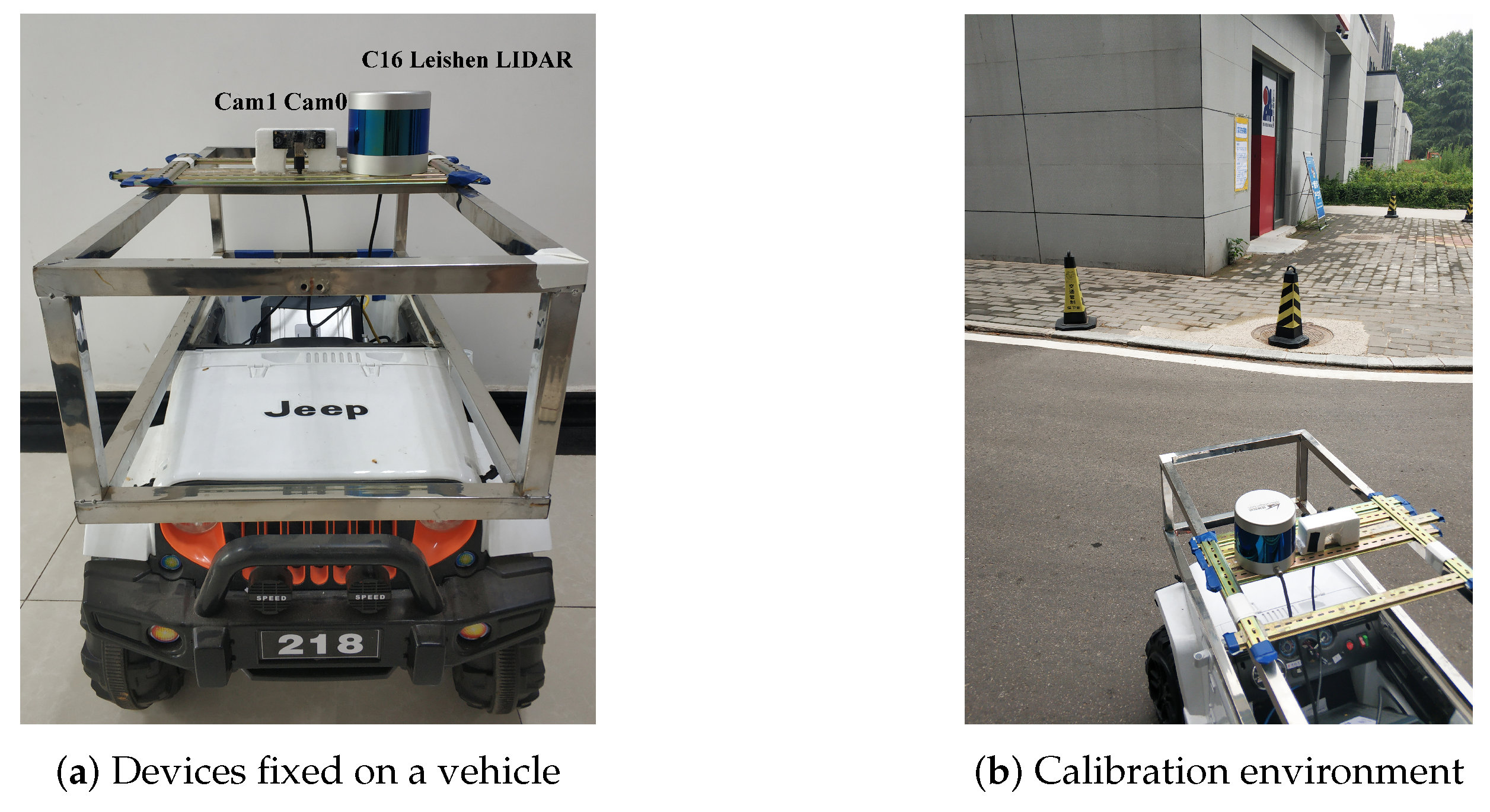
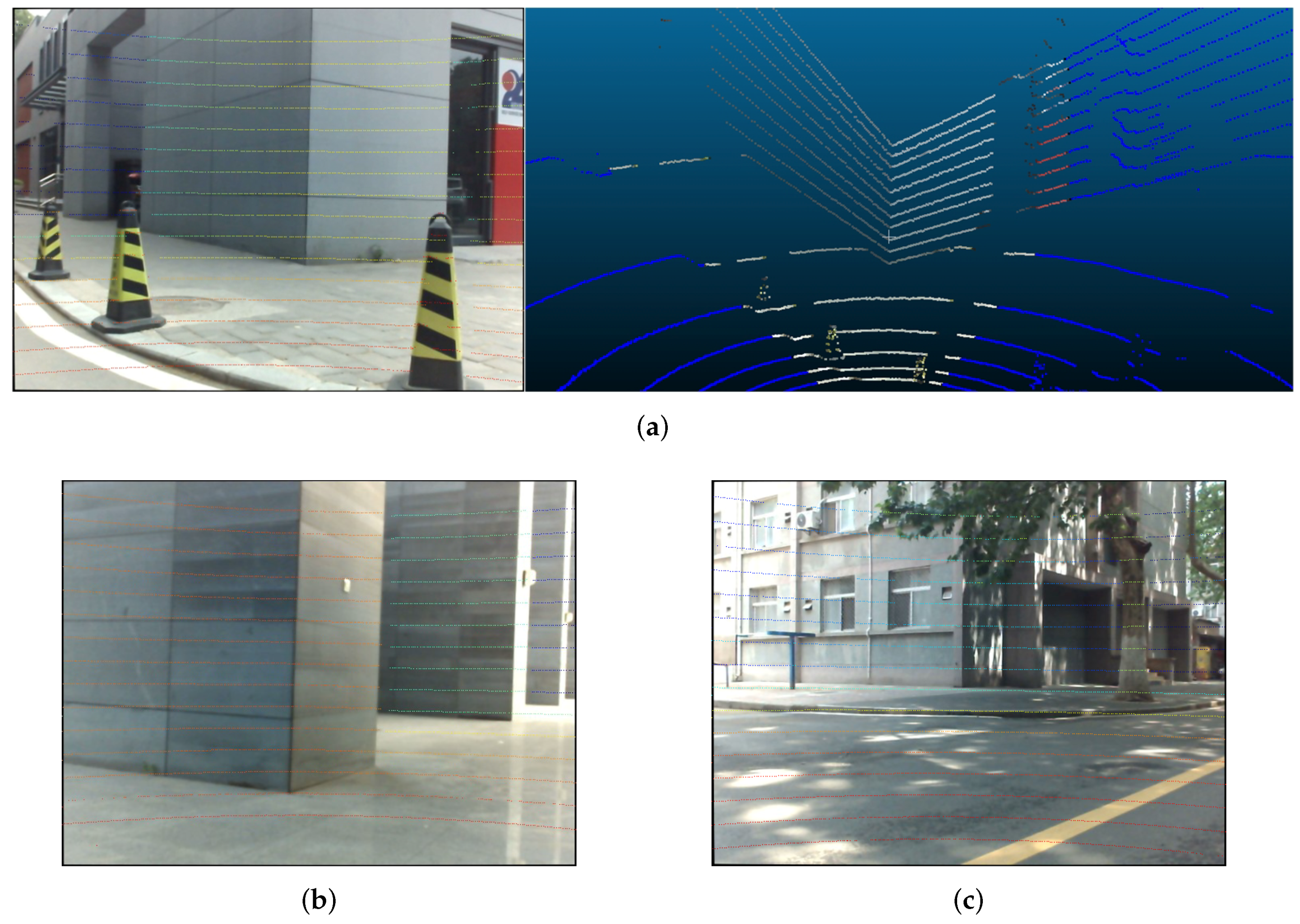
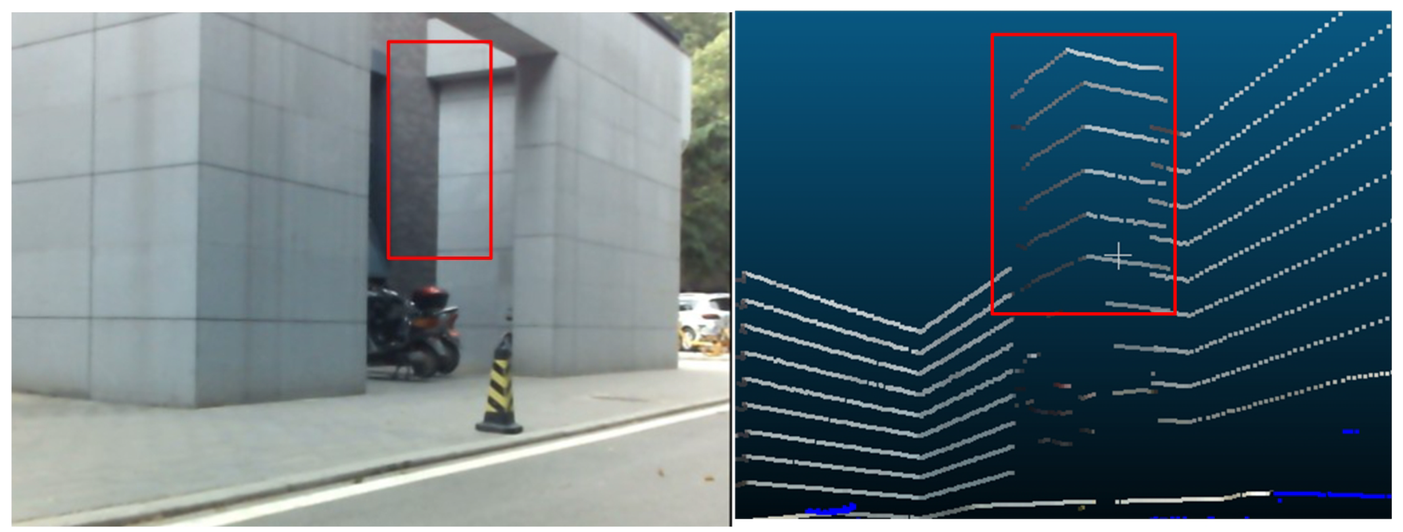
4.2. Real Data
5. Conclusions
Author Contributions
Funding
Conflicts of Interest
References
- Zhang, Q.; Pless, R. Extrinsic calibration of a camera and laser range finder (improves camera calibration). In Proceedings of the 2004 IEEE/RSJ International Conference on Intelligent Robots and Systems (IROS) (IEEE Cat. No. 04CH37566), Sendai, Japan, 28 September–2 October 2004; Volume 3, pp. 2301–2306. [Google Scholar]
- Fremont, V.; Rodriguez Florez, S.A.; Bonnifait, P. Circular targets for 3d alignment of video and lidar sensors. Adv. Robot. 2012, 26, 2087–2113. [Google Scholar]
- Gomez-Ojeda, R.; Briales, J.; Fernandez-Moral, E.; Gonzalez-Jimenez, J. Extrinsic calibration of a 2D laser-rangefinder and a camera based on scene corners. In Proceedings of the 2015 IEEE International Conference on Robotics and Automation (ICRA), Seattle, WA, USA, 26–30 May 2015; pp. 3611–3616. [Google Scholar]
- Taylor, Z.; Nieto, J. Motion-based calibration of multimodal sensor extrinsics and timing offset estimation. IEEE Trans. Robot. 2016, 32, 1215–1229. [Google Scholar]
- Park, C.; Moghadam, P.; Kim, S.; Sridharan, S.; Fookes, C. Spatiotemporal camera-LiDAR calibration: A targetless and structureless approach. IEEE Robot. Autom. Lett. 2020, 5, 1556–1563. [Google Scholar]
- Schneider, N.; Piewak, F.; Stiller, C.; Franke, U. RegNet: Multimodal sensor registration using deep neural networks. In Proceedings of the 2017 IEEE intelligent vehicles symposium (IV), Los Angeles, CA, USA, 11–14 June 2017; pp. 1803–1810. [Google Scholar]
- Iyer, G.; Ram, R.K.; Murthy, J.K.; Krishna, K.M. CalibNet: Geometrically supervised extrinsic calibration using 3D spatial transformer networks. In Proceedings of the 2018 IEEE/RSJ International Conference on Intelligent Robots and Systems (IROS), Madrid, Spain, 1–5 October 2018; pp. 1110–1117. [Google Scholar]
- Scaramuzza, D.; Harati, A.; Siegwart, R. Extrinsic self calibration of a camera and a 3d laser range finder from natural scenes. In Proceedings of the 2007 IEEE/RSJ International Conference on Intelligent Robots and Systems, San Diego, CA, USA, 29 October–2 November 2007; pp. 4164–4169. [Google Scholar]
- Moghadam, P.; Bosse, M.; Zlot, R. Line-based extrinsic calibration of range and image sensors. In Proceedings of the 2013 IEEE International Conference on Robotics and Automation, Karlsruhe, Germany, 6–10 May 2013; pp. 3685–3691. [Google Scholar]
- Xu, C.; Zhang, L.; Cheng, L.; Koch, R. Pose estimation from line correspondences: A complete analysis and a series of solutions. IEEE Trans. Pattern Anal. Mach. Intell. 2016, 39, 1209–1222. [Google Scholar] [PubMed]
- Wang, P.; Xu, G.; Cheng, Y. A novel algebraic solution to the perspective-three-line pose problem. Comput. Vis. Image Underst. 2020, 191, 102711. [Google Scholar]
- Huang, L.; Barth, M. A novel multi-planar LIDAR and computer vision calibration procedure using 2D patterns for automated navigation. In Proceedings of the 2009 IEEE Intelligent Vehicles Symposium, Xi’an, China, 3–5 June 2009; pp. 117–122. [Google Scholar]
- Vasconcelos, F.; Barreto, J.P.; Nunes, U. A minimal solution for the extrinsic calibration of a camera and a laser-rangefinder. IEEE Trans. Pattern Anal. Mach. Intell. 2012, 34, 2097–2107. [Google Scholar]
- Geiger, A.; Moosmann, F.; Car, Ö.; Schuster, B. Automatic camera and range sensor calibration using a single shot. In Proceedings of the 2012 IEEE International Conference on Robotics and Automation, Saint Paul, MN, USA, 14–18 May 2012; pp. 3936–3943. [Google Scholar]
- Zhou, L. A new minimal solution for the extrinsic calibration of a 2D LIDAR and a camera using three plane-line correspondences. IEEE Sens. J. 2013, 14, 442–454. [Google Scholar]
- Zhou, L.; Li, Z.; Kaess, M. Automatic extrinsic calibration of a camera and a 3d lidar using line and plane correspondences. In Proceedings of the 2018 IEEE/RSJ International Conference on Intelligent Robots and Systems (IROS), Madrid, Spain, 1–5 October 2018; pp. 5562–5569. [Google Scholar]
- Chai, Z.; Sun, Y.; Xiong, Z. A Novel Method for LiDAR Camera Calibration by Plane Fitting. In Proceedings of the 2018 IEEE/ASME International Conference on Advanced Intelligent Mechatronics (AIM), Auckland, New Zealand, 9–12 July 2018; pp. 286–291. [Google Scholar]
- Verma, S.; Berrio, J.S.; Worrall, S.; Nebot, E. Automatic extrinsic calibration between a camera and a 3D Lidar using 3D point and plane correspondences. In Proceedings of the 2019 IEEE Intelligent Transportation Systems Conference (ITSC), Auckland, New Zealand, 9–12 July 2019; pp. 3906–3912. [Google Scholar]
- An, P.; Ma, T.; Yu, K.; Fang, B.; Zhang, J.; Fu, W.; Ma, J. Geometric calibration for LiDAR-camera system fusing 3D-2D and 3D-3D point correspondences. Opt. Express 2020, 28, 2122–2141. [Google Scholar]
- Li, G.; Liu, Y.; Dong, L.; Cai, X.; Zhou, D. An algorithm for extrinsic parameters calibration of a camera and a laser range finder using line features. In Proceedings of the 2007 IEEE/RSJ International Conference on Intelligent Robots and Systems, San Diego, CA, USA, 29 October–2 November 2007; pp. 3854–3859. [Google Scholar]
- Willis, A.R.; Zapata, M.J.; Conrad, J.M. A linear method for calibrating LIDAR-and-camera systems. In Proceedings of the 2009 IEEE International Symposium on Modeling, Analysis & Simulation of Computer and Telecommunication Systems, London, UK, 21–23 September 2009; pp. 1–3. [Google Scholar]
- Kwak, K.; Huber, D.F.; Badino, H.; Kanade, T. Extrinsic calibration of a single line scanning lidar and a camera. In Proceedings of the 2011 IEEE/RSJ International Conference on Intelligent Robots and Systems, London, UK, 21–23 September 2011; pp. 3283–3289. [Google Scholar]
- Naroditsky, O.; Patterson, A.; Daniilidis, K. Automatic alignment of a camera with a line scan lidar system. In Proceedings of the 2011 IEEE International Conference on Robotics and Automation, Shanghai, China, 9–13 May 2011; pp. 3429–3434. [Google Scholar]
- Pusztai, Z.; Hajder, L. Accurate calibration of LiDAR-camera systems using ordinary boxes. In Proceedings of the IEEE International Conference on Computer Vision Workshops, Venice, Italy, 22–29 October 2017; pp. 394–402. [Google Scholar]
- Dong, W.; Isler, V. A novel method for the extrinsic calibration of a 2D laser rangefinder and a camera. IEEE Sens. J. 2018, 18, 4200–4211. [Google Scholar]
- Forkuo, E.; King, B. Registration of Photogrammetric Imagery and Laser Scanner Point Clouds. In Proceedings of the Mountains of data, peak decisions, 2004 ASPRS Annual Conference, Denver, CO, USA, 23–28 May 2004; p. 58. [Google Scholar]
- Forkuo, E.K.; King, B. Automatic fusion of photogrammetric imagery and laser scanner point clouds. Int. Arch. Photogramm. Remote Sens. 2004, 35, 921–926. [Google Scholar]
- Mirzaei, F.M.; Roumeliotis, S.I. Globally optimal pose estimation from line correspondences. In Proceedings of the 2011 IEEE International Conference on Robotics and Automation, Shanghai, China, 9–13 May 2011; pp. 5581–5588. [Google Scholar]
- Levinson, J.; Thrun, S. Automatic Online Calibration of Cameras and Lasers. In Proceedings of the 2013 MIT Press Robotics: Science and Systems, Berlin, Germany, 24–28 June 2013; Volume 2. [Google Scholar]
- Tamas, L.; Kato, Z. Targetless calibration of a lidar-perspective camera pair. In Proceedings of the IEEE International Conference on Computer Vision Workshops, Sydney, Australia, 1–8 December 2013; pp. 668–675. [Google Scholar]
- Pandey, G.; McBride, J.R.; Savarese, S.; Eustice, R.M. Automatic extrinsic calibration of vision and lidar by maximizing mutual information. J. Field Robot. 2015, 32, 696–722. [Google Scholar]
- Xiao, Z.; Li, H.; Zhou, D.; Dai, Y.; Dai, B. Accurate extrinsic calibration between monocular camera and sparse 3D lidar points without markers. In Proceedings of the 2017 IEEE Intelligent Vehicles Symposium (IV), Los Angeles, CA, USA, 11–14 June 2017; pp. 424–429. [Google Scholar]
- Jiang, J.; Xue, P.; Chen, S.; Liu, Z.; Zhang, X.; Zheng, N. Line feature based extrinsic calibration of LiDAR and camera. In Proceedings of the 2018 IEEE International Conference on Vehicular Electronics and Safety (ICVES), Los Angeles, CA, USA, 11–14 June 2018; pp. 1–6. [Google Scholar]
- Bileschi, S. Fully automatic calibration of lidar and video streams from a vehicle. In Proceedings of the 2009 IEEE 12th International Conference on Computer Vision Workshops, ICCV Workshops, Kyoto, Japan, 27 September–4 October 2009; pp. 1457–1464. [Google Scholar]
- Schneider, S.; Luettel, T.; Wuensche, H.J. Odometry-based online extrinsic sensor calibration. In Proceedings of the 2013 IEEE/RSJ International Conference on Intelligent Robots and Systems, Tokyo, Japan, 3–7 November 2013; pp. 1287–1292. [Google Scholar]
- Gallego, G.; Lund, J.E.; Mueggler, E.; Rebecq, H.; Delbruck, T.; Scaramuzza, D. Event-based, 6-DOF camera tracking from photometric depth maps. IEEE Trans. Pattern Anal. Mach. Intell. 2017, 40, 2402–2412. [Google Scholar]
- Yuan, K.; Guo, Z.; Wang, Z.J. RGGNet: Tolerance Aware LiDAR-Camera Online Calibration with Geometric Deep Learning and Generative Model. IEEE Robot. Autom. Lett. 2020, 5, 6956–6963. [Google Scholar]
- Zhang, Z. A flexible new technique for camera calibration. IEEE Trans. Pattern Anal. Mach. Intell. 2000, 22, 1330–1334. [Google Scholar]
- Hartley, R.; Zisserman, A. Multiple View Geometry in Computer Vision; Cambridge University Press: Cambridge, UK, 2003. [Google Scholar]
- Zhou, Y.; Qi, H.; Ma, Y. End-to-end wireframe parsing. In Proceedings of the IEEE International Conference on Computer Vision, Seoul, Korea, 27 October–2 November 2019; pp. 962–971. [Google Scholar]
- Rother, C. A new approach to vanishing point detection in architectural environments. Image Vis. Comput. 2002, 20, 647–655. [Google Scholar]
- Tardif, J.P. Non-iterative approach for fast and accurate vanishing point detection. In Proceedings of the 2009 IEEE 12th International Conference on Computer Vision, Kyoto, Japan, 29 September–2 October 2009; pp. 1250–1257. [Google Scholar]
- Zhai, M.; Workman, S.; Jacobs, N. Detecting vanishing points using global image context in a non-manhattan world. In Proceedings of the IEEE Conference on Computer Vision and Pattern Recognition, Las Vegas, NV, USA, 26 June–1 July 2016; pp. 5657–5665. [Google Scholar]
- Nurunnabi, A.; Belton, D.; West, G. Robust segmentation in laser scanning 3D point cloud data. In Proceedings of the 2012 International Conference on Digital Image Computing Techniques and Applications (DICTA), Fremantle, WA, Australia, 3–5 December 2012; pp. 1–8. [Google Scholar]
- Vo, A.V.; Truong-Hong, L.; Laefer, D.F.; Bertolotto, M. Octree-based region growing for point cloud segmentation. ISPRS J. Photogramm. Remote Sens. 2015, 104, 88–100. [Google Scholar]
- Xu, B.; Jiang, W.; Shan, J.; Zhang, J.; Li, L. Investigation on the weighted ransac approaches for building roof plane segmentation from lidar point clouds. Remote Sens. 2016, 8, 5. [Google Scholar]
- Fischler, M.A.; Bolles, R.C. Random sample consensus: A paradigm for model fitting with applications to image analysis and automated cartography. Commun. ACM 1981, 24, 381–395. [Google Scholar]
- Zhang, C.; Zhang, Z. Calibration between depth and color sensors for commodity depth cameras. In Computer Vision and Machine Learning with RGB-D Sensors; Springer: Berlin/Heidelberg, Germany, 2014; pp. 47–64. [Google Scholar]
- Arun, K.S.; Huang, T.S.; Blostein, S.D. Least-squares fitting of two 3-D point sets. IEEE Trans. Pattern Anal. Mach. Intell. 1987, 9, 698–700. [Google Scholar]
- Zhang, X.; Zhang, Z.; Li, Y.; Zhu, X.; Yu, Q.; Ou, J. Robust camera pose estimation from unknown or known line correspondences. Appl. Opt. 2012, 51, 936–948. [Google Scholar]
- Dhome, M.; Richetin, M. Determination of the attitude of 3D objects from a single perspective view. IEEE Trans. Pattern Anal. Mach. Intell. 1989, 11, 1265–1278. [Google Scholar]
- Brown, K.M.; Dennis, J. Derivative free analogues of the Levenberg-Marquardt and Gauss algorithms for nonlinear least squares approximation. Numer. Math. 1971, 18, 289–297. [Google Scholar]
- Blender Sensor Simulation. Available online: https://www.blensor.org/ (accessed on 26 May 2020).


| 1800 | 1800 | 960 | 540 |
| Cam0 | ||||
| Cam1 |
| mm | mm | mm |
| LiDAR to Cam0 | Confidence | LiDAR to Cam1 | Confidence | |
|---|---|---|---|---|
| Translation (m) | ||||
| Rotation (axis-angle) | ||||
| Pandey [31] | m | m | m | |||
| proposed | m | m | m |
Publisher’s Note: MDPI stays neutral with regard to jurisdictional claims in published maps and institutional affiliations. |
© 2020 by the authors. Licensee MDPI, Basel, Switzerland. This article is an open access article distributed under the terms and conditions of the Creative Commons Attribution (CC BY) license (http://creativecommons.org/licenses/by/4.0/).
Share and Cite
Bai, Z.; Jiang, G.; Xu, A. LiDAR-Camera Calibration Using Line Correspondences. Sensors 2020, 20, 6319. https://doi.org/10.3390/s20216319
Bai Z, Jiang G, Xu A. LiDAR-Camera Calibration Using Line Correspondences. Sensors. 2020; 20(21):6319. https://doi.org/10.3390/s20216319
Chicago/Turabian StyleBai, Zixuan, Guang Jiang, and Ailing Xu. 2020. "LiDAR-Camera Calibration Using Line Correspondences" Sensors 20, no. 21: 6319. https://doi.org/10.3390/s20216319
APA StyleBai, Z., Jiang, G., & Xu, A. (2020). LiDAR-Camera Calibration Using Line Correspondences. Sensors, 20(21), 6319. https://doi.org/10.3390/s20216319